Themed Section: Engineering and Technology
Hybrid Image Compression using orthogonal wavelets
P.M.K.Prasad*1, G.B.S.R. Naidu2, Ch.Babji Prasad3, D.Srinivasa Rao4
*1,2,3,4 Department of ECE, GMR Institute of Technology, Rajam, Andhra Pradesh, India
ABSTRACT
In this paper, a new algorithm is introduced for analyzing images in a better way based on the design of wavelets. Wavelet algorithms process data at different scales or resolutions. They have advantages over traditional fourier methods in analyzing physical situations where the signal contains discontinuities and sharp spikes. The fundamental idea behind wavelets is to analyze according to scale. To construct a wavelet of some practical utility, we rarely start by drawing a waveform. Instead, it usually makes more sense to design the appropriate quadrature mirror filters, and then use them to create the waveform. Here, later case is used to design the wavelet and Lossless predictive coding used to compress the image. Proposed hybrid algorithm gives better results, especially in getting less entropy values.
Keywords
JPEG2000, Discrete Wavelet Transform (DWT), & Lossless Predictive coding
I. INTRODUCTION
There are many applications requiring image compression, such as multimedia, internet, satellite imaging, remote sensing, and preservation of art work, etc. Decades of research in this area has produced a number of image compression algorithms. Most of the effort extended over the past decades on the image compression has been directed towards the application and analysis of orthogonal transforms. The orthogonal transform exhibits a number of properties that make it useful. First, it generally conforms to a parseval constraint in that energy present in the image is same as that displayed in the image‟s transform. Second, the transform coefficients bear no resemblance to the image and many of the coefficients are small and, if discarded, will provide for image compression with nominal degradation of the reconstructed image. Third, certain sub scenes of interest, such as some targets or particular textures, have easily recognized signatures in the transform domain [1]. The
Discrete Wavelet Transform has attracted
widespread interest as a method of information coding.
Since the mid-80s, members from both the International Telecommunication Union (ITU) and the International Organization for Standardization (ISO) have been working together to establish a joint international standard for the compression of grayscale and color still images. This effort has been known as JPEG, the Joint Photographic Experts Group the “joint” in JPEG refers to the collaboration between ITU and ISO). After evaluating a number of coding schemes, the JPEG members selected a DCT (Discrete Cosine Transform) based method. JPEG became a Draft International Standard (DIS) in 1991 and an International Standard (IS) in 1992 [2][3][4][5].
With the continual expansion of multimedia and Internet applications, the needs and requirements of the technologies used, grew and evolved. In March 1997 a new call for contributions were launched for the development of a new standard for the
compression of still images, the JPEG2000 [6] [7]. This, was intended to create a new image coding system for different types of still images (bi-level, gray-level, color, multi-component), with different characteristics (natural images, scientific, medical, remote sensing, text, rendered graphics, etc) allowing different imaging models (client/server, real-time transmission, image library archival, limited buffer and bandwidth resources, etc) preferably within a unified system. The committee members selected a DWT based method. JPEG2000 became an IS in 2000 [8].
This paper is organized as follows: In Section I the history of DWT is described. The Wavelet theory is explained in Section II. The proposed algorithm is explained in Section III. Finally, some comparative results are shown in Section IV of the paper, while in Section V, the conclusion of the paper is discussed.
II. METHODS AND MATERIAL
2.1 Wavelet Theory
Frequency domain analysis using fourier transform is extremely useful for analyzing the signal because the signal‟s frequency content is very important for understanding the nature of signal and the noise that contaminates it. The only drawback is, loss of time information. When looking at a fourier transform of signal, it is impossible to tell when a particular event took place. So to overcome this drawback, the same transform was adapted to analyze only a small window of the signal at a time. This technique is known as short time fourier transform which maps a signal into a two dimensional function of time and frequency to get the localized point information but the only drawback is that, the window size is same for all frequencies. Many signals require more flexible approach that is flexible window size. This technique is known as wavelet transform.. It allows the different window sizes for different frequencies. It allows the use of long time intervals for more-precise low frequency
information and short time interval for high – frequency information. The major advantage of wavelets is the ability to perform localized area of a larger signal.
A wavelet is a “small wave”, which has its energy concentrated in time to give a tool for the analysis of transient, non-stationary, or time-varying phenomena. wavelet analysis is about analyzing signal with short duration finite energy functions. They transform the signal under investigating into another representation which presents the signal in a more useful form.
Fig. 1 Sine wave and Wavelet (db 10)
It still has the oscillating wave-like characteristic but also has the ability to allow simultaneous time and frequency analysis with a flexible mathematical foundation. Wavelet transform is widely used in image processing. Wavelet transform of a signal means to describe the signal with a family of functions.
Sinusoids are smooth and predictable; wavelets tend to be irregular and asymmetric. Just looking at pictures of wavelets and sine waves, you can see intuitively that signals with sharp changes might be better analyzed with an irregular wavelet than with a smooth sinusoid. Just as some foods are better handled with a fork than a spoon.
The wavelet transform of continuous time signal is known as continuous wavelet transform (CWT) and is defined as[1]
dt a
b x x f a x f
x a Wf
R b
a
* ( ) 1 ( ) ( )
) ,
( ,
(1)
Where ( )
1 ) ( ,
a b x a x b a
where, „a‟ is the scaling parameter, and „b‟ is the time shift parameter. The signal x(t) is transformed by analyzing function ( )
a b x
The analyzing function is not limited to complex exponential as used in the fourier transform. In fact, the only restriction is that, it must be short and oscillatory. This restriction ensures that the integral in the above equation is finite and hence the name wavelet or small wave was given to this transform
Generally speaking, binary wavelet transform is
often used in digital image processing, so a=2j. If the signal is an image, the one dimension wavelet transform should be extended to two-dimensional wavelet transform. For a two-dimensional function
f(x, y), the wavelet transform is
) , ( * ) , ( ) ,
(x y f x y , x y
f
WS ab (2)
Where,*expresses the convolution along different direction, s is the scale. In two-dimensional images, the intensity of edges can be enhanced in each one-dimensional image by convolving.
If the window of the images is convolved in the x
direction over an image, a peak will result at positions where an edge is aligned with the y
direction. This operation is approximately like taking the first derivative of the image intensity function with respect to x or y. The wavelet
transform of f(x, y) under the condition of 2j is expressed as
) , ( * ) , ( ) , (
) , ( * ) , ( ) , (
2 2
2 2
y x y
x f y x f W
y x y
x f y x f W
j j
j j
y y
x x
(3)
A wavelet is a waveform of effectively limited duration that has an average value of zero.
A. DWT analysis and synthesis
Wavelet analysis can be used to divide the information of an image into approximation and
detail sub signals[9].The best way to describe discrete wavelet transform is through a series of cascaded filters. We first consider the FIR-based discrete transform. The input image X is fed into a low-pass filter h‟ and a high-pass filter g‟ separately. The output of the two filters are then sub sampled, resulting low-pass sub band yL and high-pass sub band yH.
Fig. 2 DWT analysis and synthesis system
The original signal can be reconstructed by synthesis filters h and g which take the up sampled yL and yH as inputs [9]. To perform the forward DWT the standard uses a 1-D sub band decomposition of a 1-D set of samples into low-pass samples and high-low-pass samples. Low low-pass samples represent a down sampled low-resolution version of the original set. High-pass samples represent a down sampled residual version of the original set, needed for the perfect reconstruction of the original set from the low-pass set.
Fig. 3 2D DWT analysis filter bank
B. Design of Wavelets
modified wavelet filters are used to compute the DWT.
(a) (b)
(c) (d)
Fig. 4 Original & Modified Wavelet filters
(a) Haar (b) DB4 (c) Sym4 (d) Bior6.8
2.2 Proposed algorithm
The implementation of hybrid method for image compression for different images is a novel
algorithm. The hybrid method for image
compression algorithm is as follows:
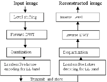
1. Level Shifting:
In the level shifting step a value of 128 is subtracted from each and every pixel to get the level shifted image as
g(m, n) = f(m, n) – 128.
2. Computation of 2D-DWT of the level shifted image.
3. Performing Quantization of the DWT matrix based on the energy in the sub band.
4. Lossless predictive coding is applied to LL band.
Fig 5: Block diagram of hybrid image compression
A. Lossless Predictive Coding
Predictive coding is an image compression technique which uses a compact model of an image to predict pixel values of an image based on the values of neighboring pixels. A model of an image is a function model(x; y), which computes (predicts) the pixel value at coordinate (x; y) of an image, given the values of some neighbors of pixel (x; y), where neighbors are pixels whose values are known. Typically, when processing an image in raster scan order (left to right, top to bottom), neighbors are selected from the pixels above and to the left of the current pixel. For example, a common set of neighbors used for predictive coding is the set {(x-1, y-1), (x, y- 1),(x+1, y-1), (x-1, y)}. Linear predictive coding is a simple, special case of predictive coding in which the model simply takes the difference of the neighboring values. There are two expected sources of compression in predictive coding based image compression (assuming that the predictive model is accurate enough). First, the coded image for each pixel should have a smaller magnitude than the corresponding pixel in the original image (therefore requiring fewer bits to transmit the coded image). Second, the coded image should have less entropy than the original message, since the model should remove many of the “principal components” of the image. To complete
the compression, the quantized image is
compressed using an entropy coding algorithm such as Huffman coding or arithmetic coding or proposed algorithm. If we transmit this compressed coded image then a receiver can reconstruct the original image by applying an analogous decoding procedure [10][11]. The bi-orthogonal wavelets can be applied not only to image compression but also for edge detection [12].
1 1.5 2 -0.5
0 0.5 1 1.5 2
1 2 3 4 5 -0.1
0 0.1 0.2 0.3 0.4 0.5 0.6 0.7
0 2 4 6 8 -0.2
-0.1 0 0.1 0.2 0.3 0.4 0.5 0.6 0.7 0.8
0 5 10 15 -0.2
-0.1 0 0.1 0.2 0.3 0.4 0.5 0.6 0.7
0 2 4 6 8 -0.1
0 0.1 0.2 0.3 0.4 0.5 0.6 0.7 0.8 0.9
0 5 10 15 -0.1
0 0.1 0.2 0.3 0.4 0.5 0.6 0.7
0 5 10 15 20 -0.1
0 0.1 0.2 0.3 0.4 0.5 0.6 0.7 0.8 0.9
0 10 20 30 -0.1
III. RESULTS AND DISCUSSION
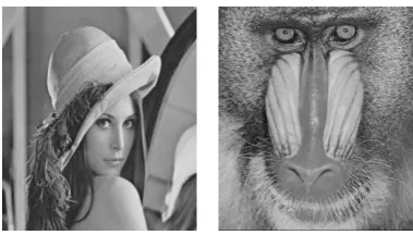
Experiments are performed on gray level images to verify the proposed method. These 3images are represented by 8 bits/pixel and size is 512 x 512 images used for experiments are shown in Fig.6
Fig. 6 Images (Lena, & Mandrill)
The entropy (E) is defined as
∑
where s is the set of processed coefficients and p(e) is the probability of processed coefficients. By using entropy, number of bits required for compressed image is calculated and is shown in Table 1( for lena image) and Table 2( for Mandrill image). Here, n is the level of decomposition.
TABLE 1
TABLE 2
The Reconstructed images after applying the compression mechanism using various wavelets is shown in the Fig 7 for single level decomposition
Fig. 7 Reconstructed Images (Lena, & Mandrill) for n=1
IV.CONCLUSION
The proposed hybrid image compression using orthogonal wavelets is giving better compression compared to wavelet image compression. Results are superior with modified sym4 wavelet when compared with other wavelets. Better quantization and prediction may further improve the results. The Proposed hybrid algorithm gives less entropy.
V. REFERENCES
[1] Z. Fan and R. D. Queiroz. Maximum likelihood estimation of JPEG quantization table in the identification of Bitmap Compression. IEEE, 948-951, 2000.
[2] Charilaos Christopoulos, Athanassios Skodras, Touradj Ebrahimi,”The JPEG2000 still Image coding system: An overview”. IEEE, 1103-1127, November 2000.
[3] G. K. Wallace, “The JPEG Still Picture Compression Standard”, IEEE Trans. Consumer Electronics, Vol. 38, No 1, Feb. 1992.
[4] W. B. Pennebaker and J. L. Mitcell, “JPEG: Still Image Data Compression Stndard”, Van Nostrand Reinhold, 1993.
[5] V. Bhaskaran and K. Konstantinides, “Image and Video Compression Standards: Algorithms and Applications”, 2nd Ed., Kluwer Academic Publishers.
[6] ISO/IEC JTC1/SC29/WG1 N505, “Call for contributions for JPEG 2000 (JTC 1.29.14, 15444):Image Coding System,” March 1997.
[7] ISO/IEC JTC1/SC29/WG1 N390R, “New work item: JPEG 2000 image coding system,” March 1997.
[8] M. Boliek, C. Christopoulos and E. Majani (editors), “JPEG2000 Part I Final Draft International Standard,” (ISO/IEC FDIS15444-1), ISO/IEC JTC1/SC29/
[9] P.M.K. Prasad, Prabhakar.Telegarapu, G. Uma Madhuri,” Image Compression using Orthogonal Wavelets viewed from Peak Signal to Noise Ratio and Computation time”International Journal of Computer Applications (0975 – 888) Volume 47– No.4, June 2012,,P.P.28-34 [10] T. Acharya and A. K. Ray, Image Processing: Principles and
Applications. Hoboken, NJ: John Wiley & Sons, 2005
[11] Alex Fukunaga and Andre Stechert, Evolving Nonlinear Predictive Models for Lossless Image Compression with Genetic Programming,
[12] S.Devendra,, P.M.K.Prasad, “Lifting Bi-orthogonal Wavelet Transform Based Edge Feature Extraction” International Journal of Advanced Trends in Computer Science and Engineering, ISSN 2278-3091, Vol.3 , No.5, Pages : 68- 71 (2014).
without proposed without proposed without proposed without proposed 1 3.6404 2.5967 3.3876 2.3971 3.386 2.3926 3.3187 2.1665 2 2.0081 1.6355 1.7423 1.3024 1.7373 1.301 1.729 1.1247 3 1.1919 1.0481 1.026 0.7883 1.0314 0.7985 1.072 0.7002 4 0.7325 0.6618 0.6625 0.535 0.6639 0.5415 0.7482 0.495 5 0.4542 0.4308 0.4525 0.3786 0.4508 0.3908 0.551 0.3801 6 0.2808 0.2801 0.3135 0.2759 0.3089 0.2875 0.4239 0.3096
BIOR6.8 LENA.GIF
n filters ↓ →
HAAR DB4 SYM4
without proposed without proposed without proposed without proposed 1 4.8615 3.8618 4.7359 4.0308 4.7465 4.0326 4.685 3.3905 2 3.435 2.6022 3.3266 2.8102 3.3338 2.8116 3.3519 2.1126 3 2.2841 1.6375 2.2515 1.8501 2.2521 1.8571 2.3536 1.3052 4 1.3995 0.9207 1.4328 1.1572 1.4328 1.1564 1.5951 0.7741 5 0.7767 0.4982 0.8454 0.6733 0.8433 0.683 1.0204 0.4867 6 0.4124 0.2849 0.4918 0.4013 0.4911 0.4066 0.6562 0.3217 n filters
↓ →
HAAR DB4 SYM4 BIOR6.8