Abstract—Array synthesis is usually done by controlling amplitude and phase levels or element spacing functions of the array to get the desired characteristics of the radiation pattern. This paper addresses the problem of designing thinned linear arrays with practical radiating elements dipoles to achieve lowest side lobe level. Traditional methods are not well suited for thinning large arrays; hence Genetic algorithm(GA) is used to find the optimum thinned configuration to achieve the specified sidelobe level .The computed patterns are compared with the uniform array patterns for different number of elements.
Index Terms—Thinning, Array synthesis, Dipole arrays, Genetic Algorithm
I. INTRODUCTION
In most of the communication and radar applications, it is necessary to design a highly directional antenna with low sidelobes. So, it is preferred to choose array antennas that have high gain and directivity compared to individual radiating elements [1]. In array of identical radiating elements, overall pattern can be designed by varying amplitude level, phase level and space distribution of elements [2]. Low sidelobes can be obtained through carefully amplitude weighting the signals received at each element. An alternative for large arrays is space tapering [3]. Space tapering produces the low-sidelobe amplitude taper by making the element density proportional to the desired amplitude taper at a particular location on the array [4]. One approach is aperiodic or non uniform spacing of the elements. Non uniformly spaced elements generate a low-sidelobe amplitude taper by placing equally weighted elements in such a way that the spacing of the elements creates a tapered excitation across the aperture.
A second approach is the thinned array [5].Thinning means turning off some elements in a uniformly spaced or periodic array. In case of large array with ‘P’ number of elements, the possible thinning combinations are 2P [6]. So, checking all the combinations to find the optimum configuration is very laborious.A numerical optimization approach was first tried in 1964 [7]. Dynamic programming provided a numerical optimization method to find the lowest sidelobe level of a thinned array. The binary GA is a natural for this problem and was one of the first uses of a GA in antenna design [8]. Hence,
Manuscript received September 13, 2011; revised October 12, 2011. V. Rajya Lakshmi is with the Anil Neerukonda Institute of Technology and Sciences, Visakhapatnam, AP 531162 India (e-mail: [email protected]).
G. .S. N. Raju, was with Andhra University, Visakhapatnam, AP 530003 INDIA. He is now The Principal, Andhra University College of Engineering (Autonomous), Visakhaptanam, AP 530003 India (e-mail: [email protected]).
one of the non gradient based optimization methods, Genetic algorithm is used to find the optimum layout of the linear array of dipoles. Genetic algorithms are successfully applied in electromagnetic radiation problems especially thinned arrays. [9-12]. The main concern of the paper is to find the best arrangement of linear array of dipoles which can give relative side lobe level as low as possible without enhancing the null to null beam width.
II. GENETIC ALGORITHM
Genetic algorithms are a part of evolutionary computing, which is a rapidly growing area of artificial intelligence. Genetic algorithms are inspired by Darwin's theory of evolution. Simply said, problems are solved by an evolutionary process resulting in a best solution. The Algorithm begins with a set of solutions (represented by chromosomes) called population. Solutions from one population are taken and used to form a new population. This is motivated by a hope, that the new population will be better than the old one. Solutions which are then selected to form new solutions (offspring) are selected according to their fitness - the more suitable they are the more chances they have to reproduce. This is repeated until some condition (for example number of populations or improvement of the best solution) is satisfied. The outline of the Genetic algorithm is given below.
1) [Start] Generate random population of n chromosomes (appropriate solutions for the problem).
2) [Fitness] Evaluate the fitness g(x) of each chromosome x in the population.
3) [New population] Create a new population by repeating following steps until the new population is complete.
a. [Selection] Select two parent chromosomes from a population according to their fitness (the better fitness, the higher chance to be selected). b. [Crossover] with a crossover probability cross over the parents to form new offspring (children). If no crossover performed, offspring is the exact copy of parents.
c. [Mutation] with a mutation probability mutate new offspring at each locus (position in chromosome).
4) [Replace] Use new generated population for a further run of the algorithm.
5) [Test] If the end condition is satisfied, stop, and return the best solution in current population.
6) [Loop] Go to step 2.
Chromosomes are selected from the population to be parents for crossover. The problem is how to select these chromosomes. According to Darwin's theory of evolution the
Optimization of Thinned Dipole Arrays Using Genetic
Algorithm
best ones survive to create new offspring. There are many methods in selecting the best chromosomes. Examples are roulette wheel selection, Boltzmann selection, tournament selection, rank selection, steady state selection and some others. From the genetic algorithm outline, the crossover and mutation are the most important parts of the genetic algorithm. The performance is influenced mainly by these two operators:
A) Crossover operates on selected genes from parent chromosomes and creates new offspring. The simplest way how to do that is to choose randomly some crossover point and copy everything before this point from the first parent and then copy everything after the crossover point from the other parent.
B) After a crossover is performed, mutation takes place. Mutation is intended to prevent falling of all solutions in the population into a local optimum of the solved problem. Mutation operation randomly changes the offspring resulted from crossover. In case of binary encoding we can switch a few randomly chosen bits from 1 to 0 or from 0 to 1.
Genetic algorithms differ from most optimization methods, because it has the following characteristics [13].
1) It works with a coding of the parameters, not the parameters themselves.
2) It searches from many points instead of a single point. 3) It doesn’t use derivatives.
4) It uses random transition rules, not deterministic rules.
III. ARRAY OF DIPOLE AND GA
Among the most common radiators dipole is one, which consists of a straight conductor (often a thin wire) broken at some point where it is excited by a voltage derived from a transmission line. In most cases the exciting source is at the centre. Here the dipole resonate at λ/2 length. The radiating elements in the array of present interest are considered to be dipoles spaced d=λ/2 apart. A symmetric linear array is shown in Fig.1. Radiation from an array of dipoles using multiplicative theory is array factor*element pattern.The far field characteristics of continuous line source are evaluated using the radiation integral [14].
Fig. 1. Geometry of 2N element symmetric linear array.
∑
=−
=
Nn j
n
e
k
n
du
A
E
n1
cos[
(
0
.
5
)
]
2
)
(
θ
ϕ (1)Here,
k=wave number= 2π/λ, λ=wave length. An = Amplitude of the nth element. Φn= phase of the nth element.
d=spacing between the radiating elements. θ= angle between the line of observer and broadside.
u= sinθ,
The fitness function associated with this array is the maximum SLL of its associated far field pattern to be minimized. The general form of the fitness function is given by
(
maxE( ))
)) ) ( E ( log 20 ( Max Fitness
0 10
θ θ
= (2) ο
≠ θ π ≤ θ ≤ π
− /2 /2, 0
IV. ELEMENT PATTERN OF HALF WAVE DIPOLE
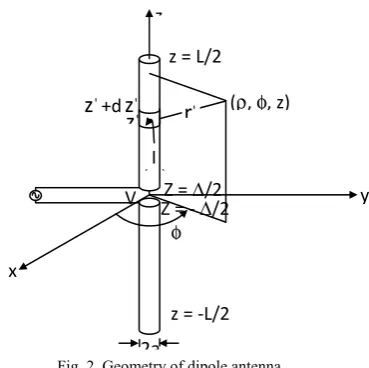
The radiation pattern obtained is valid for any length of the dipole, provided it is centre-fed. This method is found to provide a simple expression for current distribution. It is also possible to use the method of moments [15] to determine the current distribution when the elements of interest are thick and long. Consider a linear antenna in the form of a cylindrical perfect conductor of length ‘L’ and radius ‘a’ as shown in fig. 2.
Fig. 2. Geometry of dipole antenna.
It is driven by a voltage ‘V’ across a narrow gap at the centre, which extends fromZ=−Δ 2 toZ=Δ 2. As a result, a current (Iz′)flows along the antenna, producing electromagnetic fields E and H in the space surrounding the antenna.
The electric field E outside the antenna is derivable
entirely from the vector magnetic potential ‘A’ as follows
A
E = −∇φ− jω (3) Since ∇⋅A =−jεjωφ (4) We have
[
]
( )
⎥ ⎥ ⎦ ⎤ ⎢
⎢ ⎣ ⎡
+ ∇ ∇
⎟ ⎠ ⎞ ⎜ ⎝ ⎛
ω ω =
ω − ∇ ∇ ωμε =
A A
A A
E
. v
j
j ) . ( j
1
2 o
(5)
(ρ, φ, z)
V
2a x
z = L/2
φ
Z = ∆/2 y
Z = - ∆/2
'
r
zz = -L/2
'
z
'
z
+dz
'I
As the element is Z-direcrted, A has only a Z-component.
The Z-component of (3) is
⎟ ⎟ ⎠ ⎞ ⎜ ⎜ ⎝ ⎛ + ∂ ∂ ω −
= 2z 2 z
2
2
z k A
Z A k
j
E (6)
The quantity Ez is equal to zero except at the gap. Across the gap, which we assume to be infinitesimally narrow, we can write
( )
z VEz =− δ (7)
Hence k A j V
( )
zZ A z 2 2 z 2 δ ωμε = + ∂
∂ (8)
where k2=ω2με
The right hand side of (6) is equal to zero except across the gap. Thus the solution for Az at points outside the gap is given by kz sin C kz cos C
Az = 1 + 2 (9) For a symmetrically fed antenna
) z (I ) z
(I ′ = − ′ (10) and Az(z′)= Az(−z′) (11)
Then (7) becomes
( )
kz sin C kz cos CAz = 1 + 2 (12) To satisfy the condition at the gap, we integrate (6) across the gap i.e., from = − Δ
2 1
Z to = Δ
2 1
Z obtaining
V j zA
k z
A z 12
2 1 z z 2 2 1 z 2 1 z
z + = ωμε
∂ ∂ = Δ Δ − = Δ = Δ − = (13)
In the limit of an infinitesimal gap, Δ→0 and we find that, for (10) to satisfy (6), we must have
c 2 jV k 2 V j
C2= ωμε = (14)
Hence
( )
sin( )
kzc 2 jV cos kz cos C
Az = 1 + (15)
We know that A can also be expressed in terms of an
integral of the current on the antenna. At a point with cylindrical coordinates (ρ, φ, and z).
' 2 / L 2 / L ' Z dz r ) jkr exp( ) z (I 4 ∫ − π μ = −
A (16)
where r= ρ2+
(
z−z')
2 (17)On the surface of the antennaρ=a, r= ρ2+
(
z−z')
2and
( )
(
)
(
)
' 2 L 2 L 2 ' 2 2 2 ' z dz z z a ' z z a jk exp z I4 ∫ + −
⎥⎦ ⎤ ⎢⎣ ⎡− + − π μ = −
A (18)
Equating (13) and (16), there results
( )
(
)
(
)
( )
sin( )
k zC 2 jV kz cos C dz z z a z z a jk exp z I 4 1 ' 2 L 2
L 2 ' 2
2 ' 2 ' + = ∫ − + ⎥⎦ ⎤ ⎢⎣ ⎡− + − π μ
− (19)
Equation (17) is Hall en’s integral equation for the current distribution in the case when the conductivity of the antenna is assumed to be infinite. The problem is to find a function of
z′ forIsuch that the equation is satisfied. The remaining constant C1 is to be determined by the boundary condition
( )
z' 0I = at z'=±L2 .
Various approximate methods have been derived to solve the integral equation of Hallen. By using the quantity
( )
La ln 21 1
=
Ω (20)
As a small parameter and solves the equation in successive powers of1Ω. The result is
( )
⎟ ⎟ ⎟ ⎟ ⎠ ⎞ ⎜ ⎜ ⎜ ⎜ ⎝ ⎛ − − + Ω + Ω + ⎟ ⎠ ⎞ ⎜ ⎝ ⎛ − − + Ω + Ω + ⎟ ⎠ ⎞ ⎜ ⎝ ⎛ − Ω = − − − − 2 2 1 1 2 2 1 1 ' ' d d kL 2 1 cos b b z L 2 1 sin 60 jV z I (21)where b1, b2, d1, d2 ... etc are functions of L and Z. for very thin antenna, Ω is very large and
( )
⎟ ⎟ ⎟ ⎟ ⎠ ⎞ ⎜ ⎜ ⎜ ⎜ ⎝ ⎛ ⎟ ⎠ ⎞ ⎜ ⎝ ⎛ ⎥⎦ ⎤ ⎢⎣ ⎡ − Ω = kL 2 1 cos z L 2 1 k sin 60 jV z I '' (22)
On setting ⎟ ⎠ ⎞ ⎜ ⎝ ⎛ Ω ≡ kL 2 1 cos 60 jV
Im (23)
( )
⎥ ⎦ ⎤ ⎢ ⎣ ⎡ ⎟ ⎠ ⎞ ⎜ ⎝ ⎛ −= m '
' L z
2 1 k sin I z
I (24)
( )
⎟ ⎠ ⎞ ⎜ ⎝ ⎛ × ⎥ ⎦ ⎤ ⎢ ⎣ ⎡ ⎟ ⎠ ⎞ ⎜ ⎝ ⎛ − = kL 2 1 cos a L ln 2 60 z L 2 1 k sin jV ' (25)The far field electric and magnetic field components due to differential length dz′is
( )
' ' dz R 4 sin z jkI d π θ = φH (26)
φ θ =ηH E
d
Far field approximations are
θ −
≈r zcos
R ' for phase terms
r
R≈ for amplitude terms Provided ⎟⎟
⎠ ⎞ ⎜ ⎜ ⎝ ⎛ λ ≥2 L2 r
Equation (24) can be written as
dz e R 4 sin ) ' z ( jkI
d φ jkz'cosθ
π θ =
H (27)
By integrating the (25), we get the total field
( )
∫ π θ = ∫ = − θ − φ φ 2 L 2 L ' cos ' jkz 2 L 2L 4 r Iz'e dz
sin jk
dH
H (28)
For a very thin dipole, and for a center-fed antenna with a sinusoidal current distribution is
( )
( )( ) z 0
e z 2 L k sin I 0 z e z 2 L k sin I z I ' kr t j ' m ' kr t j ' m ' < ⎥ ⎦ ⎤ ⎢ ⎣ ⎡ ⎟ ⎠ ⎞ ⎜ ⎝ ⎛ + = > ⎥ ⎦ ⎤ ⎢ ⎣ ⎡ ⎟ ⎠ ⎞ ⎜ ⎝ ⎛ − = − ω − ω (29)
Using the (27), the (26) Hφcan be written as
( ) ⎪⎭ ⎪ ⎬ ⎫ ∫ ⎥ ⎦ ⎤ ⎢ ⎣ ⎡ ⎟ ⎠ ⎞ ⎜ ⎝ ⎛ − + ⎪⎩ ⎪ ⎨ ⎧ ∫ ⎥ ⎦ ⎤ ⎢ ⎣ ⎡ ⎟ ⎠ ⎞ ⎜ ⎝ ⎛ + π θ = θ − θ − ω φ 2 L 0 ' cos ' jkz ' ' 0 2 L cos ' jkz ' kr t j m dz e z 2 L k sin dz e z 2 L k sin r 4 e sin jkI H (30) After integration and simplification, the (28) becomes
( ) ⎥ ⎥ ⎥ ⎥ ⎦ ⎤ ⎢ ⎢ ⎢ ⎢ ⎣ ⎡ θ ⎟ ⎠ ⎞ ⎜ ⎝ ⎛ − ⎟ ⎠ ⎞ ⎜ ⎝ ⎛ θ π = ω−
φ sin 2
kL cos cos 2 kL cos r 2 e
jI j t kr
m
H (31)
The total Eθcomponent can be written as
( ) ⎥ ⎥ ⎥ ⎥ ⎦ ⎤ ⎢ ⎢ ⎢ ⎢ ⎣ ⎡ θ ⎟ ⎠ ⎞ ⎜ ⎝ ⎛ − ⎟ ⎠ ⎞ ⎜ ⎝ ⎛ θ π η = ω−
θ sin 2
kL cos cos 2 kL cos r 2 e I
j m j t kr
E
(32)
V. RESULTS
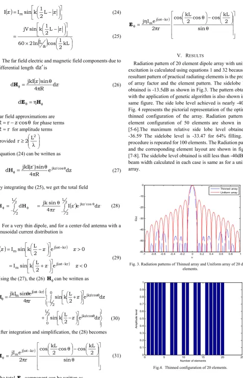
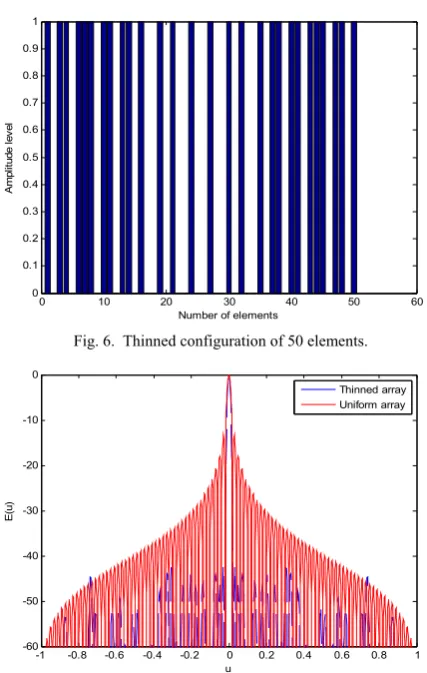
Radiation pattern of 20 element dipole array with uniform excitation is calculated using equations 1 and 32 because the resultant pattern of practical radiating elements is the product of array factor and the element pattern. The sidelobe level obtained is -13.5dB as shown in Fig.3. The pattern obtained with the application of genetic algorithm is also shown in the same figure. The side lobe level achieved is nearly -40 dB. Fig. 4 represents the pictorial representation of the optimum thinned configuration of the array. Radiation pattern and element configuration of 50 elements are shown in figs. [5-6].The maximum relative side lobe level obtained is -36.59. The sidelobe level is -33.47 for 64% filling. The procedure is repeated for 100 elements. The Radiation pattern and the corresponding element layout are shown in figures [7-8]. The sidelobe level obtained is still less than -40dB.The beam width calculated in each case is same as for a uniform array.
Fig. 3. Radiation patterns of Thinned array and Uniform array of 20 dipole elements.
Fig.4. Thinned configuration of 20 elements.
-1 -0.8 -0.6 -0.4 -0.2 0 0.2 0.4 0.6 0.8 1 -60 -50 -40 -30 -20 -10 0 u E(u ) Thinned array Uniform array
0 5 10 15 20 25
0 0.1 0.2 0.3 0.4 0.5 0.6 0.7 0.8 0.9 1
Number of elements
Fig. 5. Radiation patterns of Thinned array and Uniform array of 50 elements.
Fig. 6. Thinned configuration of 50 elements.
Fig. 7.Comparision of Radiation patterns of Thinned array and Uniform array of 100 elements.
Fig. 8. Thinned configuration of 100 elements.
VI. CONCLUSION
The thinned arrays provide cost effective solution
compared to the uniform arrays. The application of genetic algorithm for optimization of radiation pattern characteristics of thinned arrays is found to be very useful, because with less number of dipoles, the side lobe level is reduced from -13.5dB to about -35dB. The algorithm is found to be accurate and fast and the patterns are converged after 30 iterations. It is also evident from the results; the beam width of the main beam remains unaltered while reducing the side lobe level. It is also possible to extend the algorithm for other parameters of the arrays.
REFERENCES
[1] G. S. N. Raju, Antennas and Propagation, Pearson Education, 2005.
[2] R. S. Elliot, Antenna Theory and Design, Prentice-Hall, New Jersey
1981.
[3] R. L. Haupt, “Synthesizing low sidelobe quantized amplitude and phase tapers for linear arrays using genetic algorithms,” in Proc. Inte. Conf. Electromagnetics in Advanced Applications, Torino, Italy, Sept. 1995, pp.221-224.
[4] P. Lopez, J. A. Rodriguez, F. Ares, and E. Moreno, “Low sidelobe level in almost uniformly excited arrays,” IEE Electron. Letters, pp.
1991-1993, Nov 2000.
[5] J. F. Deford and O. P. Gandhi, “Phase only synthesis of minimum peak side lobe patterns for linear and planar arrays,” IEEE Trans. Anten. Propag., pp. 191-201, Feb. 1988.
[6] R. L.Haupt, “Thinned Arrays using Genetic Algorithms,” IEEE Trans on Antennas and Propagation, vol. 42, no. 7, July 1994.
[7] R. L. Haupt, “Optimum quantized low side lobe phase tapers for arrays,”
IEE Electronic Letters, pp. 1117-1118, July 1995.
[8] D. W. Boeringer and D. H. Werner, “Adaptive mutation parameter toggling genetic algorithm for phase only array synthesis,” IEE Electron. Letters, pp. 1618-1619, Dec. 2002.
[9] R. L. Haupt, “An Introduction to Genetic Algorithm for
Electromagnetics,” IEEE Antennas and Propagation Magazine, vol. 37,
no. 2, pp. 7-15, April 1995.
[10] J. Johnson, Y. Rahmat-Samii, “Genetic algorithm optimization and its application to antenna design,” IEEE AP-SInternational Symposium,
vol. 1, pp. 326-329, Seattle, June 19-24, 1994.
[11] J. M. Johnson, and Y. Rahmat-Samii, “Genetic Algorithms in Engineering Electromagnetics,” IEEE Antennas and propagation Magazine,vol. 39, no. 4, April 1997.
[12] F. Soltankarini, J. Nourinia, and Ch. Ghobadi, “Side Lobe Level Optimization in Phased Array Antennas Using Genetic Algorithm,” presented at the ISSTA2004, Sydney, Australia, 30 Aug - 2 Sept. 2004. [13] D. E. Goldberg, Genetic Algorithms, New York: Addison-Wesley,
1999, ch1. 4.
[14] C. A. Balanis, Antenna Theory Analysis and Design, 2nd Edition, John
Willy & Sons Inc, New York, 1997.
[15] R. F. Harrington, Time –Harmonic Electromagnetic Fields,
McGraw-Hill, New York, pp. 110-112, 1961.
Rajya Lakshmi Valluri is working as Associate
professor in Anil Neerukonda Institute of Technology and Sciences, Visakhapatnam and pursuing Ph.D in Electronics and communications Engineering..
G.S.N.Raju is Professor of Electronics and
Communication Engineering since 1994, Principal, Andhra University College of Engineering (Autonomous), Andhra University. Chief Editor, Journal of Electromagnetic Compatibility. Guided 22
Ph.D.s in Electronics and Communication
Engineering. He has published more than 200 Research Papers in National and International journals / Conferences proceedings.
-1 -0.8 -0.6 -0.4 -0.2 0 0.2 0.4 0.6 0.8 1 -60
-50 -40 -30 -20 -10 0
u
E(
u)
Thinned array uniform array
0 10 20 30 40 50 60
0 0.1 0.2 0.3 0.4 0.5 0.6 0.7 0.8 0.9 1
Number of elements
A
m
plit
ud
e le
ve
l
-1 -0.8 -0.6 -0.4 -0.2 0 0.2 0.4 0.6 0.8 1 -60
-50 -40 -30 -20 -10 0
u
E(
u)
Thinned array Uniform array
0 20 40 60 80 100 120
0 0.1 0.2 0.3 0.4 0.5 0.6 0.7 0.8 0.9 1
Number of elements
Am
pl
itude l
ev