R E S E A R C H
Open Access
Efficient algorithms for training the parameters
of hidden Markov models using stochastic
expectation maximization (EM) training and
Viterbi training
Tin Y Lam, Irmtraud M Meyer
*Abstract
Background:Hidden Markov models are widely employed by numerous bioinformatics programs used today. Applications range widely from comparative gene prediction to time-series analyses of micro-array data. The parameters of the underlying models need to be adjusted for specific data sets, for example the genome of a particular species, in order to maximize the prediction accuracy. Computationally efficient algorithms for parameter training are thus key to maximizing the usability of a wide range of bioinformatics applications.
Results:We introduce two computationally efficient training algorithms, one for Viterbi training and one for stochastic expectation maximization (EM) training, which render the memory requirements independent of the sequence length. Unlike the existing algorithms for Viterbi and stochastic EM training which require a two-step procedure, our two new algorithms require only one step and scan the input sequence in only one direction. We also implement these two new algorithms and the already published linear-memory algorithm for EM training into the hidden Markov model compiler HMM-CONVERTER and examine their respective practical merits for three small example models.
Conclusions:Bioinformatics applications employing hidden Markov models can use the two algorithms in order to make Viterbi training and stochastic EM training more computationally efficient. Using these algorithms, parameter training can thus be attempted for more complex models and longer training sequences. The two new algorithms have the added advantage of being easier to implement than the corresponding default algorithms for Viterbi training and stochastic EM training.
Background
Hidden Markov models (HMMs) and their variants are widely used for analyzing biological sequence data. Bioinformatics applications range from methods for comparative gene prediction (e.g. [1,2]) to methods for modeling promoter grammars (e.g. [3]), identifying pro-tein domains (e.g. [4]), predicting propro-tein interfaces (e.g. [5]), the topology of transmembrane proteins (e.g. [6]) and residue-residue contacts in protein structures (e.g. [7]), querying pathways in protein interaction networks (e.g. [8]), predicting the occupancy of transcription
factors (e.g. [9]) as well as inference models for genome-wide association studies (e.g. [10]) and disease associa-tion tests for inferring ancestral haplotypes (e.g. [11]).
Most of these bioinformatics applications have been set up for a specific type of analysis and a specific biolo-gical data set, at least initially. The states of the underly-ing HMM and the implemented prediction algorithms determine which type of data analysis can be performed, whereas the parameter values of the HMM are chosen for a particular data set in order to optimize the corre-sponding prediction accuracy. If we want to apply the same method to a new data set, e.g. predict genes in a different genome, we need to adjust the parameter values in order to make sure the performance accuracy is optimal.
* Correspondence: [email protected]
Centre for High-Throughput Biology, Department of Computer Science and Department of Medical Genetics, 2366 Main Mall, University of British Columbia, Vancouver V6T 1Z4, Canada
Manually adjusting the parameters of an HMM in order to get a high prediction accuracy can be a very time consuming task which is also not guaranteed to improve the performance accuracy. A variety of training algorithms have therefore been devised in order to address this challenge. These training algorithms require as input and starting point a so-called training set of (typically partly annotated) data. Starting with a set of (typically user-chosen) initial parameter values, the training algorithm employs an iterative procedure which subsequently derives new, more refined parameter values. The iterations are stopped when a termination criterion is met, e.g. when a maximum number of itera-tions have been completed or when the change of the log-likelihood from one iteration to the next become sufficiently small. The model with the final set of para-meters is then used to test if the performance accuracy has been improved. This is typically done by analyzing a
test setof annotated data which has no overlap with the training set by comparing the predicted to the known annotation.
Of the training algorithms used in bioinformatics applications, the Viterbi training algorithm [12,13] is probably the most commonly used, see e.g. [14-16]. This is due to the fact that it is easy to implement if the Viterbi algorithm [17] is used for generating predictions. In each iteration of Viterbi training, a new set of para-meter valuesjis derived from the counts of emissions and transitions in the Viterbi paths Π* for the set of training sequences . Because the new parameters are completely determined by the Viterbi paths, Viterbi training converges as soon as the Viterbi paths no longer change or, alternatively, if a fixed number of iterations have been completed. Viterbi training finds at best a local optimum of the likelihood P( , Π*|j), i.e. it derives parameter values jthat maximize the contri-bution from the set of Viterbi pathsΠ*to the likelihood. There already exist a number of algorithms that can make Viterbi decoding computationally more efficient. Keibleret al. [18] introduce two heuristic algorithms for Viterbi decoding which they implement into the gene-prediction program TWINSCAN/N-SCAN, called “Treeterbi” and “Parallel Treeterbi”, which have the same worst case asymptotic memory and time require-ments as the standard Viterbi algorithm, but which in practice work in a significantly more memory efficient way. Srameket al. [19] present a new algorithm, called “on-line Viterbi algorithm”which renders Viterbi decod-ing more memory efficient without significantly increas-ing the time requirement. The most recent contribution is from Lifshits et al. [20] who propose more efficient algorithms for Viterbi decoding and Viterbi training. These new algorithms exploit repetitions in the input
sequences (in five different ways) in order to accelerate the default algorithm.
Another well-known training algorithm for HMMs is Baum-Welch training [21] which is an expectation max-imization (EM) algorithm [22]. In each iteration, a new set of parameter values is derived from the estimated number of counts of emissions and transitions by con-sidering allpossible state paths (rather than only a sin-gle Viterbi path) for every training sequence. The iterations are typically stopped after a fixed number of iterations or as soon as the change in the log-likelihood is sufficiently small. For Baum-Welch training, the likeli-hood P( |j) [13] can be shown to converge (under some conditions) to a stationary point which is either a local optimum or a saddle point. Baum-Welch training using the traditional combination of forward and back-ward algorithm [13] is, for example, implemented into the prokaryotic gene prediction method EASYGENE [23] and the HMM-compiler HMMoC [15]. As for Viterbi training, the outcome of Baum-Welch training may strongly depend on the chosen set of initial para-meter values. As Jensen [24] and Khreich et al. [25] describe, computationally more efficient algorithms for Baum-Welch training which render the memory requirement independent of the sequence length have been proposed, first in the communication field by [26-28] and later, independently, in bioinformatics by Miklós and Meyer [29], see also [30]. The advantage of this linear-memory memory algorithm is that it is com-paratively easy to implement as it requires only a one-rather than a two-step procedure and as it scans the sequence in a uni- rather than bi-directional way. This algorithm was employed by Hobolth and Jensen [31] for comparative gene prediction and has also been imple-mented, albeit in a modified version, by Churbanov and Winters-Hilt [30] who also compare it to other imple-mentations of Viterbi and Baum-Welch training includ-ing checkpointinclud-ing implementations.
Stochastic expectation maximization (EM) training or Monte Carlo EM training [32] is another iterative proce-dure for training the parameters of HMMs. Instead of considering only a singleViterbi state path for a given training sequence as in Viterbi training or all state paths as in Baum-Welch training, stochastic EM training considers a fixed-number ofKstate paths Πswhich are sampled from the posterior distribution P(Π|X) for every training sequence X in every iteration. Sampled state paths have already been used in several bioinfor-matics applications for sequence decoding, see e.g. [2,33] where sampled state paths are used in the context of gene prediction to detect alternative splice variants.
can be combined with the traditional check-pointing algorithm [34-36] in order to trade time for memory requirements.
We here introduce two new algorithms that make Viterbi training and stochastic EM training computa-tionally more efficient. Both algorithms have the signifi-cant advantage of rendering the memory requirement independent of the sequence length for HMMs while keeping the time requirement the same (for Viterbi training) or modifying it by a factor ofM K/(M +K), i. e. decreasing it when only one state path K = 1 is sampled for a model of M states (for stochastic EM training). Both algorithms are inspired by the linear-memory algorithm for Baum-Welch training which requires only a uni-directional rather than bi-directional movement along the input sequence and which has the added advantage of being considerably easier to imple-ment. We present a detailed description of the two new algorithms for Viterbi training and stochastic EM train-ing. In addition, we implement all three algorithms, i.e. the new algorithms for Viterbi training and stochastic EM training and the previously published linear-memory algorithm for Baum-Welch training, into our HMM-compiler HMM-CONVERTER[37] and examine the practical features of these these three algorithms for three small example HMMs.
Methods and Results Definitions and notation
In order to simplify the notation in the following, we will assume without loss of generality that we are deal-ing with a 1st-order HMM where the Startstate and the Endstate are the only silent states. Our description of the existing and the new algorithms easily generalize to higher-order HMMs, HMMs with more silent states (provided there exists no circular path in the HMM involving only silent states) and n-HMMs, i.e. HMMs which readnun-aligned input sequences rather than a single input sequence at a time. An HMM is defined by
● a set of states = {0, 1, ... , M}, where state 0 denotes thestart and stateM denotes theEnd state and where all other states are non-silent,
●a set of transition probabilities = {ti,j|i,jÎ},
where ti,j denotes the transition probability to go
from stateito state jand
∑
j S∈ ti j, =1 for every stateiÎ and
● a set of emission probabilitiesℰ= {ei(y)|i Î,y
Î}, where ei(y) denotes the emission probability
of state i for symbol y and
∑
y∈e yi( )=1 for everynon-silent state iÎ and denotes the alphabet from which the symbols in the input sequences are
derived, e.g. ={A, C, G, T}when dealing with DNA sequences.
We also define:
●Tmaxis the maximum number of states that any
state in the model is connected to, also called the model’s connectivity.
● = {X1,X2, ... ,XN} denotes the training set ofN
sequences, where each particular training sequence
Xi of length Li is denoted Xi =( ,x x1i i2,…,xLii). In the following and to simplify the notation, we pick one particular training sequenceXÎ of lengthL
as representative which we denoteX= (x1,x2, ... ,xL).
We writeXn= (x1,x2, ... ,xn),nÎ{1, ... ,L}, to denote
the sub-sequence ofX which finishes at sequence positionn.
●Π= (π0, π1, ... , πL+1) denotes a state path in the HMM for an input sequenceX of lengthL, i.e. state
πi is assigned to sequence position xi. Π*denotes a
Viterbi path and Πs a state path that has been sampled from the posterior distributionP(Π|X ) of the corresponding sequenceX.
A linear-memory algorithm for Viterbi training
Of the HMM-based methods that provide automatic algorithms for parameter training, Viterbi training [13] is the most popular. This is primarily due to the fact that Viterbi training is readily implemented if the Viterbi algorithm is used to generate predictions. Similar to Baum-Welch training [21,22], Viterbi training is an iterative training procedure. Unlike Baum-Welch train-ing, however, which considers allstate paths for a given training sequence in each iteration, Viterbi training only considers a single state path, namely a Viterbi path, when deriving new sets of parameters. In each iteration, a new set of parameter values is derived from the counts of emissions and transitions in the Viterbi paths [17] of the training sequences. The iterations are terminated as soon as the Viterbi paths of the training sequences no longer change.
In the following,
●let E y Xiq( , ,Π*( ))X denote the number of times
that stateireads symbolyfrom input sequence Xin Viterbi pathΠ*(X) given the HMM with parameters from theq-th iteration,
●in particular let E y Xiq( , k,Π*(Xk,k*=m)) denote
from input sequence X in the partial Viterbi path Π*(X , * m) ( *, , * , * m)
k k = = 0 …k−1k = which finishes
at sequence positionkin statem, and
● let Ti jq,( ,X Π*( ))X denote the number of times that a transition from state i to state jis used in Viterbi path Π*(X) for sequenceX given the HMM with parameters from theq-th iteration,
● in particular let Ti jq,(Xk,Π*(Xk,*k=m)) denote the number of times that a transition from stateito state j is used in the partial Viterbi path
Π*(X , * m) ( *, , * , * m)
k k = = 0 …k−1k = which finishes
at sequence positionkin statem.
In the following, the superscriptq will indicate from which iteration the underlying parameters derive. If we consider all Nsequences of a training set = {X1, ...
XN} and a Viterbi pathΠ*(Xn) for each sequenceXn in the training set, the recursion which updates the values of the transition and emission probabilities reads:
t
T X X
T X X
i jq
i j
q n n
n N
i jq n n
n N
j M ,
, *
, *
( , ( ))
( , ( ))
+ =
= =
=
∑
∑
∑
1 1
1 1
Π
Π (1)
e y
E y X X
E y X X
i
q i
q n n
n N
iq n n
n N
y
+ =
= ∈
=
∑
∑
∑
1 1
1
( )
( , , ( ))
( ’, , ( ))
*
* ’
Π
Π
(2)
These equations assume that we know the values of
Ti jq,(Xn,Π*(Xn)) and E y Xiq( , n,Π*(Xn)), i.e. how often each transition and emission is used in the Viterbi path Π*
(Xn) for training sequenceXn.
One straightforward way to determine Ti jq,(Xn,Π*(Xn)) and E y Xiq( , n,Π*(Xn)) is to first calculate the two-dimensional Viterbi matrix for every training sequence
Xn, to then derive a Viterbi state pathΠ*(Xn) from each Viterbi matrix using the well-known traceback procedure [17] and to then simply count how often each transition and each emission was used. Using this strategy, every iteration in the Viterbi training algorithm would require (M maxi{Li} + maxi{Li}) memory and
(MTmax i L L)
N i N
i i
= =
∑
1 +∑
1 time, where i Li N=
∑
1 is the sum ofthe Nsequence lengths in the training set and maxi
{Li} the length of the longest sequence in training set .
However, for many bioinformatics applications where the number of states in the modelM is large, the connectiv-ityTmaxof the model high or the training sequences are
long, these memory and time requirements are too large to allow automatic parameter training using this algorithm.
A linear-memory version of the Viterbi algorithm, called the Hirschberg algorithm [38], has been known since 1975. It can be used to derive Viterbi paths in memory that is linearized with respect to the length of one of the input sequences while increasing the time requirement by at most a factor of two. The Hirschberg algorithm, however, only applies ton-HMMs withn≥2, i.e. HMMs which read two or more un-aligned input sequences at a time. One significant disadvantage of the Hirschberg algorithm is that it is considerably more diffi-cult to implement than the Viterbi algorithm. Only few HMM-based applications in bioinformatics actually employ it, see e.g. [1,37,39]. We will see in the following how we can devise a linear-memory algorithm for Viterbi training that does not involve the Hirschberg algorithm and that can be applied to alln-HMMs includingn= 1.
We now introduce a linear-memory algorithm for Viterbi training. The idea for this algorithm stems from the following observations:
(V1) If we consider the description of the Viterbi algo-rithm [17], in particular the recursion, we realize that the calculation of the Viterbi values can be continued by retaining only the values for the previous sequence position.
(V2) If we have a close look at the description of the traceback procedure [17], we realize that we only have to remember the Viterbi matrix elements at theprevious
sequence position in order to deduce the state from which the Viterbi matrix element at the current
sequence position and state was derived.
(V3) If we want to derive the Viterbi pathΠfrom the Viterbi matrix, we have to start at the end of the sequence in the EndstateM.
Observations (V1) and (V2) imply that local informa-tion suffices to continue the calculainforma-tion of the Viterbi matrix elements (V1) and to derive a previous state (V2) if we already are in a particular state and sequence posi-tion, whereas observation (V3) reminds us that in order to derive the Viterbi path, we have to start at theendof the training sequence. Given these three observations, it is not obvious how we can come up with a computa-tionally more efficient algorithm for training with Viterbi paths. In order to realize that a more efficient algorithm exists, one also has to also note that:
(V4) While calculating the Viterbi matrix elements in the memory-efficient way outlined in (V1), we can
(V5) In every iterationq of the training procedure, we only need to know the values of Ti jq,( ,X Π*( ))X and
E y Xiq( , ,Π*( ))X , i.e. how often each transition and
emission was used in each Viterbi state path Π*(X) for every training sequenceX, but not wherein the Viterbi matrix each transition and emission was used.
Given all observations (V1) to (V5), we can now for-mally write down an algorithm which calculates
Ti jq,( ,X Π*( ))X and E y Xiq( , ,Π*( ))X in a computation-ally efficient way which linearizes the memory require-ment with respect to the sequence length and which is also easy to implement. In order to simplify the nota-tion, we describe the following algorithm for one parti-cular training sequence Xand omit the superscript for the iteration q, as both remain the same throughout the algorithm. In the following,
●Ti,j(k,m) denotes the number of times the
transi-tion from state i to statejis used in a Viterbi state path that finishes at sequence position kin statem, ●Ei(y,k,m) denotes the number of times that statei
reads symbol yin a Viterbi state path that finishes at sequence positionkin statem,
●vi(k) denotes the Viterbi matrix element for statei
and sequence position k, i.e. vi(k) is the probability
of the Viterbi state path, i.e. the state path with the highest overall probability, that starts at the begin-ning of the sequence in the Startstate and finishes in stateias sequence positionk,
● i, j, nÎ , y Î andl Î denotes the pre-vious state from which the current Viterbi matrix element vm(k) was derived, and
● δi,j is the delta-function withδi,j = 1 fori =jand
δi,j= 0 else.
Initialization: at the start of training sequenceX = (x1, ... ,xL) and for allmÎ , set
v m
m
T m
E y m
m
i j
i
( )
( , )
( , , )
,
0 0
0
0 0
0 0
1 0
= =
≠ ⎧ ⎨ ⎩ = =
Recursion: loop over all positionskfrom 1 toLin the training sequenceX and loop, for each such sequence position k, over all statesmÎ \{0} = {1, ... ,M } and set
v k e x v k t
T k m T k l
m m k
n n n m
i j i j l
( ) ( ) { ( ) }
( , ) ( , )
,
, , ,
= ⋅ − ⋅
= − ∈+
max
1
1 ii m j
i i m i y x
E y k m E y k l
k
⋅
= − + ⋅
,
, ,
( , , ) ( , 1, )
where l denotes the state at the previous sequence positionk −1 from which the Viterbi matrix element
vm(k) for statem and sequence positionk derives, i.e.
l=arg maxn S∈{ (v kn − ⋅1) tn m, }.
Termination: at the end of the input sequence, i.e. for
k=Land form=Mthe silentEndstate, set
v L v L t
T L M T L l
E y M
n n n M
i j i j l i M j
i
( ) { ( ) }
( , ) ( , )
( ,
,
, , , ,
= ⋅
= + ⋅
∈
max
L
L M, )=E y L li( , , )
where ldenotes the state at the sequence position L
from which the Viterbi matrix elementvM (L) for the
End state M and sequence position L derives, i.e.
l=arg maxn S∈{ ( )v Ln ⋅tn M, }.
The above algorithm yields Ti j,( ,L M)=Ti jq,( ,X Π*( ))X
and E y L Mi E y Xi X
q
( , , )= ( , ,Π*( )) (and vM(L) =Pq(X, Π*
(X))), i.e. we know how often a transition from stateito state jwas used and how often symbol y was read by stateiin Viterbi state pathΠ*(X) in iterationq.
Theorem 1: The above algorithm yields Ti j,( ,L M)= Ti jq,( ,X Π*( ))X and E y L Mi E y Xi X
q
( , , )= ( , ,Π*( )).
Proof: We will prove these statements via induction with respect to the sequence positionk.
(1) Induction start atk= 0: This corresponds to the initialization step in the algorithm.Ti,j(0,m) = 0 andEi
(y, 0, m) = 0 for allm Î as any zero-length Viterbi path finishing in state mat sequence position 0 has zero transitions from state i to j and has not read any sequence symbol.
(2) Induction step k − 1 ® k for k Î {1, ...L −1} if the state at sequence position k = L is not the
End state M : This case corresponds to the recursion
in the algorithm. We assume that
Ti j,(k−1, )m =Ti j,q(Xk−1,Π*(Xk−1,k*−1=m)) and E y ki( , −1, )m =E y Xiq( , k−1,Π*(Xk−1,*k−1=m)).
We need to distinguish two cases (a) and (b). Let l
denote the state at sequence positionk−1 from which the Viterbi matrix element vm(k) for state m and
sequence position k derives, i.e.
l=arg maxn S∈{ (v kn − ⋅1) tn m, }.
●Case (a):
Emissions (i):m=iandy=xk: In this case,Ei(y,k,
m) =Ei(y,k−1,l) + 1. As we know thatEi(y,k−1,l)
is the number of times that stateireads symbolyin a Viterbi path ending in statelat sequence position
y=xkby statem=iat the next sequence positionk
in order to obtainEi(y,k,m).
Transitions (ii): l= i and m= j: In this case, Ti,j
(k,m) =Ti,j(k−1,l) + 1. As we know thatTi,j(k−1,l)
is the number of times that a transition from stateito state jis used in a Viterbi path ending in statelat sequence position k−1, we need to add 1 count for the transition from state l=ito state m=jwhich brings us from sequence positionk−1 tokin order to getTi,j(k,m).
●Case (b):
Emissions (i): m≠i ory≠xk : In this case,Ei(y, k,
m) =Ei(y, k−1, l). We know that Ei(y,k −1,l) is
the number of times that state ireads symbolyin a Viterbi path ending in statel at sequence positionk
− 1. If we go from statel at positionk −1 to state
mat positionkand read symbolxkand ifm≠iory
≠ xk , we do not need to modify the number of
counts as we know that state iat positionkdoes not read symboly, i.e.Ei(y,k, m) = Ei(y,k−1,l).
Transitions (ii): l ≠i or m ≠ j: In this case, Ti,j
(k,m) = Ti,j(k−1,l). We know thatTi,j(k−1,l) is
the number of times that a transition from stateito state j is used in a Viterbi path ending in state lat sequence position k− 1. If we make a transition from statelat positionk−1 to statemat positionk
and if l ≠ior m≠j, we do not need to modify the number of counts as we know this is not a transition from stateito statej, i.e.Ti,j(k,m) =Ti,j(k−1,l).
(3) If the state at sequence position k = L is the
EndstateM: This case corresponds to the termination step in the algorithm. As in (2), we need to distinguish two cases (a) and (b), but now only for the transition counts. Let l denote the state at sequence position L
from which the Viterbi matrix elementvM (L) for the
End state M and sequence position L derives, i.e.
l=arg maxn S∈{ ( )v Ln ⋅tn m, }.
Emissions (i):In this case,Ei(y,L, M) = Ei(y,L,l). As
we know that Ei(y, L, l) is the number of times that
state ireads symboly in a Viterbi path ending in statel
at sequence positionL, we do not need to modify this number of counts when going to the silentEndstate at the same sequence position L as silent states do not read any symbols from the input sequence. As we are now at the end of the input sequenceX and the Viterbi pathΠ*(X), we have E y L Mi( , , )=E y Xiq( , ,Π*( ))X .
●Case (a):
Transitions (i): l=iandM =j: In this case, Ti,j(L,
M) =Ti,j(L, l) + 1. As we know thatTi,j(L, l) is the
number of times that a transition from state i to
statej is used in a Viterbi path ending in state lat sequence positionL, we need to add 1 count for the transition from statel=i to the Endstate M=jat sequence position L. Note that this transition of state does not incur a change of sequence position as theEndstate is a silent state. As we are now at the end of the input sequenceX and the Viterbi pathΠ*(X), we have Ti j,( ,L M)=Ti jq,( ,X Π*( ))X . ●Case (b):
Transitions (i):l≠iorM≠j: In this case,Ti,j(L,M)
=Ti,j(L, l). We know that Ti,j(L,l) is the number
of times that a transition from statei to state j is used in a Viterbi path ending in statel at sequence positionL. If we make a transition from statel at positionLto the Endstate M at sequence position
Land ifl≠i orM ≠j, we do not make a transition from stateito statejand thus do not need to mod-ify the number of counts, i.e.Ti,j (L, M) =Ti,j(L, l).
Also in case (a), we are now at the end of the input sequence X and the Viterbi path Π*(X ) and thus have Ti j,( ,L M)=Ti jq,( ,X Π*( )).X
End of proof.
As is clear from the above description of the algo-rithm, the calculation of the vm, Ti,j and Ei values for
sequence position krequires only the respective values for the previous sequence positionk−1, i.e. the mem-ory requirement can be linearized with respect to the sequence length.
For an HMM withM states and a training sequence of lengthL and for every free parameter of the HMM that we want to train, we thus need in every iteration (M ) memory to store thevmvalues and (M)
mem-ory to store the cumulative counts for the free para-meter itself, e.g. theTi,jvalues for a particular transition
from state i to state j. For an HMM, the memory requirement of the training using the new algorithm is thus independent of the length of the training sequence.
For training one free parameter in the HMM with the above algorithm, each iteration requires (MTmaxL)
time to calculate the vm values and to calculate the
cumulative counts. IfQis the total number of free para-meters in the model and if we choose P of these para-meters to be trained in parallel, i.e. P Î {1, ...Q} and
Q/P Î N, the memory requirement increases slightly to (MP ) and the time requirement becomes
(MT LQ) P
default algorithm for Viterbi training described above with first calculates the entire Viterbi matrix and which requires (M L) memory and (TmaxLM) time to
achieve the same. Our new algorithm thus has the sig-nificant advantage of linearizing the memory require-ment with respect to the sequence length while keeping the time requirement the same, see Table 1 for a detailed overview. Our new algorithm is thus as memory efficient as Viterbi training using the Hirschberg algo-rithm, while being more time efficient, significantly easier to implement and applicable to all n-HMMs, including the casen= 1.
A linear-memory algorithm for stochastic EM training
One alternative to Viterbi training is Baum-Welch train-ing [21], which is an expectation maximization (EM) algorithm [22]. As Viterbi training, Baum-Welch train-ing is an iterative procedure. In each iteration of Baum-Welch training, the estimated number of counts for each transition and emission is derived by considering
all possible state paths for a given training sequence in the model rather than only the single Viterbi path. As discussed in the introduction, there already exists an efficient algorithm for Baum-Welch training which line-arizes the memory requirement with respect to the sequence length and which is also relatively easy to implement.
One variant of Baum-Welch training is called stochas-tic EM algorithm [32]. Unlike Viterbi training which considers only a single state path and unlike Baum-Welch training which considersall possible state paths for every training sequence, the stochastic EM algorithm derives new parameter values from afixed number ofK
state paths (each of which is denoted Πs(X)) that are sampled for each training sequence from the posterior distributionP(Π|X). Similar to Viterbi and Baum-Welch training, the stochastic EM algorithm employs an tive procedure. As for Baum-Welch training, the itera-tions are stopped once a maximum number of iteraitera-tions have been reached or once the change in the log-likeli-hood is sufficiently small.
In strict analogy to the notation we introduced for Viterbi training, E y Xiq( , ,Πs( ))X denotes the number of times that stateireads symbolyfrom input sequenceX
in a sampled state pathΠs(X) given the HMM with para-meters from theq-th iteration. Similarly, Ti jq,( ,X Πs( ))X
denotes the number of times that a transition from state
i to state jis used in a sampled state path Πs(X) for sequenceXgiven the HMM with parameters from theq -th iteration.
As usual, the superscriptqindicates from which itera-tion the underlying parameters of the HMM derive. If we consider allNsequences of the training set = {X1, ...
XN} and sampleKstate paths Πks(Xn), kÎ {1, ... K},
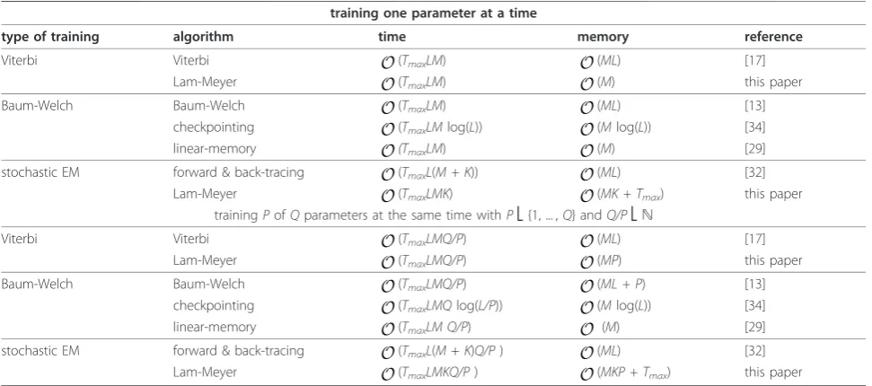
Table 1 Theoretical computational requirements
training one parameter at a time
type of training algorithm time memory reference
Viterbi Viterbi (TmaxLM) (ML) [17]
Lam-Meyer (TmaxLM) (M) this paper
Baum-Welch Baum-Welch (TmaxLM) (ML) [13]
checkpointing (TmaxLMlog(L)) (Mlog(L)) [34]
linear-memory (TmaxLM) (M) [29]
stochastic EM forward & back-tracing (TmaxL(M + K)) (ML) [32]
Lam-Meyer (TmaxLMK) (MK + Tmax) this paper
trainingPofQparameters at the same time withPÎ{1, ... ,Q} andQ/PÎN
Viterbi Viterbi (TmaxLMQ/P) (ML) [17]
Lam-Meyer (TmaxLMQ/P) (MP) this paper
Baum-Welch Baum-Welch (TmaxLMQ/P) (ML + P) [13]
checkpointing (TmaxLMQlog(L/P)) (Mlog(L)) [34]
linear-memory (TmaxLM Q/P) (M) [29]
stochastic EM forward & back-tracing (TmaxL(M+K)Q/P) (ML) [32] Lam-Meyer (TmaxLMKQ/P) (MKP + Tmax) this paper
Overview of the theoretical time and memory requirements for Viterbi training, Baum-Welch training and stochastic EM training for an HMM withMstates, a connectivity ofTmaxandQfree parameters.Kdenotes the number of state paths sampled in each iteration for every training sequence for stochastic EM training. The time and memory requirements below are the requirements per iteration for a single training sequence of lengthL. It is up to the user to decide whether to train theQfree parameters of the model sequentially, i.e. one at a time, or in parallel in groups. The two tables below cover all possibilities.
In the general case we are dealing with a training set = {X1 ,X2
, ... ,XN} ofNsequences, where the length of training sequenceXiisLi. If training involves the entire training set, i.e. all training sequences simultaneously,Lin the formulae below needs to be replaced by i Li
N
=
∑1 for the memory requirements and by maxi
{Li} for the time requirements. If, on the other hand, training is done by considering by one training sequence at a time,Lin the formulae below needs to be replaced by i Li
N
=
for each sequenceXnin the training set, the step which updates the values of the transition and emission prob-abilities can be written as:
t
T X X
T X X
i j
q i j
q n k s n k K n N
i jq n ks n
k K , , , ’ ( , ( )) ( , ( )) + = = = =
∑
∑
∑
1 1 1
1 Π Π n n N j M i q i q n
ks n
k K n N i q n e y
y X X
y X E E = = + = =
∑
∑
∑
∑
= 1 11 1 1
’
( )
( , , ( ))
( , ,
Π
′ ΠΠks n k
K
n N
y∈
∑
=∑
= (X ))∑
′ 1 1These expressions are strictly analogous to equations 1 and 2 that we introduced for Viterbi training. As before, these assume that we know the values
of Ti jq,(Xn,Πks(Xn)) and E y Xiq( , n,Πks(Xn)), i.e. how
often each transition and emission is used in each sampled state path Πks n
X
( ) for every training sequence
Xn.
Obtaining the counts from the forward algorithm and stochastic back-tracing
It is well-known that we can obtain the above countsTi,j
(X, Πs(X)) and Ei(y, X, Πs(X)) for a given training
sequence X, iterationq and a sampled state path Πs(X) by using a combination of the forward algorithm and stochastic back-tracing [13,32]. For this, we first calcu-late all values in the two-dimensional forward matrix using the forward algorithm and then invoke the sto-chastic back-tracing procedure to sample a state-pathΠs (X) from the posterior distributionP(Π|X).
We will now explain these two algorithms in detail in order to facilitate the introduction of our new algorithm. In the following,
● fi(k) denotes the sum of probabilities of all state
paths that have read training sequence X up to and including sequence positionk and that end in state
i, i.e. fi(k) = P(x1, ... , xk , s(xk ) = i), wheres(xk)
denotes the state that reads sequence position xk
from input sequence X. We call fi(k) the forward
probability for sequence position kand state i. ● pi(k,m) denotes the probability of selecting state
m as the previous state while being in state i at sequence position k (i.e. sequence position khas already been read by statei), i.e.pi(k,m) = P(πk−1=
m|πk=i). For a given sequence positionkand state
i,pi(k,m) defines a probability distribution over
pre-vious states as p k mi
m ( , )=
∑
1.The forward matrix is calculated using the forward algorithm [13]:
Initialization:at the start of the input sequence, con-sider all statesmÎ in the model and set
f m
m m( )0
1 0 0 0 = = ≠ ⎧ ⎨ ⎩
Recursion: loop over all positionskfrom 1 toLin the input sequence and loop, for each such sequence posi-tionk, over all statesmÎ \{0} = {1, ... ,M} and set
fm k em xk f kn t
n M
n m
( )= ( )⋅ ( − ⋅) ,
=
∑
0 1 (3)Termination: at the end of the input sequence, i.e. for
k = Landm = MtheEndstate, set
P X fM L f Ln t
n M
x n M
( )= ( )= ( )⋅ ,
=
∑
0Once we have calculated all forward probabilitiesfi(k)
in the two-dimensional forward matrix, i.e. for all states
i in the model and all positionskin the given training sequenceX, we can then use the stochastic back-tracing procedure [13] to sample a state path from the posterior distributionP(Π|X).
The stochastic back-tracing starts at the end of the input sequence, i.e. at sequence position k = L, in the
Endstate, i.e.i=M, and selects statemas the previous state with probability:
p k m
f k e x t
f k i
f k t
i
m k m i
i m i ( , ) ( ) ( ) ( ) ( ) , = − ⋅ ⋅ ⋅ 1
if state is not silent
m m i i
f k i
,
( ) if state is silent
⎧ ⎨ ⎪ ⎪ ⎩ ⎪ ⎪ (4)
This procedure is continued until we reach the start of the sequence and the Startstate. The resulting succes-sion of chosen previous states corresponds to one state pathΠs(X) that was sampled from the posterior distribu-tionP(Π|X).
The denominator in equation (4) corresponds to the sum of probabilities of all state paths that finish in state
i at sequence positionk, whereas the nominator corre-sponds to the sum of probabilities of all state paths that finish in state i at sequence position k and that have statemas the previous state.
When being in state iat sequence positionk, we can therefore use this ratio to sample which previous state
mwe should have come from.
time in order to first calculate the matrix of forward values and then (L) memory and (LTmax) time for
sampling a single state path from the matrix. Note that additional state paths can be sampled without having to recalculate the matrix of forward values. For samplingK
state paths for the same sequence in a given iteration, we thus need ((M + K)TmaxL) time and (ML)
memory, if we do not to store the sampled state paths themselves.
If our computer has enough memory to use the for-ward algorithm and the stochastic back-tracing proce-dure described above, each iteration in the training algorithm would require (M maxi{Li} + Kmaxi{Li})
memory and (MTmax Li K L) i
N
i i N
= =
∑
1 +∑
1 time, whereLi i N
=
∑
1 is the sum of the N sequence lengths in thetraining set and maxi{Li} the length of the longest
sequence in training set . As we do not have to keep the K sampled state paths in memory, the memory requirement can be reduced to (M maxi{Li}).
For many bioinformatics applications, however, where the number of states in the modelM is large, the con-nectivity Tmax of the model high or the training
sequences are long, these memory and time require-ments are too large to allow automatic parameter train-ing ustrain-ing stochastic EM traintrain-ing.
Obtaining the counts in a more efficient way
Our previous observations (V1) to (V5) that led to the linear-memory algorithm for Viterbi training can be replaced by similar observations for stochastic EM training:
(S1) If we consider the description of the forward algorithm above, in particular the recursion in Equation (3), we realize that the calculation of the forward values can be continued by retaining only the values for the previous sequence position.
(S2) If we have a close look at the description of the stochastic back-tracing algorithm, in particular the sam-pling step in Equation (4), we observe that the samsam-pling of a previous state only requires the forward values for the current and the previous sequence position. So, pro-vided we are at a particular sequence position and in a particular state, we can sample the state at the previous sequence position, if we know all forward values for the previous sequence position.
(S3) If we want to sample a state pathΠs(X) from the posterior distribution P(Π|X), we have to start at the
endof the sequence in theEndstate, see the description above and Equation (4) above. (The only valid alterna-tive for sampling state paths from the posterior distribu-tion would be to use the backward algorithm [13] instead of the forward algorithm and to then start the
stochastic back-tracing procedure at the start of the sequence in the Startstate.)
Observations (S1) and (S2) above imply that local information suffices to continue the calculation of the forward values (S1) and to sample a previous state (S2) if we already are in a particular state and sequence posi-tion, whereas observation (S3) reminds us that in order to sample from the correct probability distribution, we have to start the sampling at the end of the training sequence. Given these three observations, it is – as before for Viterbi training –not obvious how we can come up with a computationally more efficient algo-rithm. In order to realize that a more efficient algorithm does exist, one also has to note that:
(S4) While calculating the forward values in the mem-ory-efficient way outlined in (S1) above, we can simulta-neouslysample a previous state for every combination of a state and a sequence position that we encounter in the calculating of the forward values. This is possible because of observation (S2) above.
(S5) In every iterationqof the training procedure, we only need to know the values of Ti jq,( ,X Πs( ))X and
E y Xiq( , ,Πs( ))X , i.e. how often each transition and
emission appears in each sampled state path Πs(X) for every training sequenceX , but notwherein the matrix of forward values the transition or emission was used.
Given all observations (S1) to (S5) above, we can now formally write down a new algorithm which calculates
Ti jq,( ,X Πs( ))X and E y Xiq( , ,Πs( ))X in a computationally more efficient way. In order to simplify the notation, we consider one particular training sequenceX = (x1, ... xL)
of lengthL and omit the superscript for the iterationq, as both remain the same throughout the following algo-rithm. In the following, Ti,j(k, m) denotes the number of
times the transition from state i to state jis used in a sampled state path that finishes at sequence positionkin state mand Ei(y,k,m) denotes the number of times state
i read symbol y in a sampled state path that finishes at sequence position kin state m. As defined earlier, fi(k)
denotes the forward probability for sequence position k
and statei, pi(k, m) is the probability of selecting statem
as the previous state while being in state i at sequence positionk,i,j,nÎ andyÎ .
Initialization: at the start of the training sequenceX
and for all statesmÎ , set
f m
m
T m
E y m
m
i j
i ( )
( , )
( , , )
,
0 1 0
0 0
0 0
0 0
= =
≠ ⎧
Recursion: loop over all positionskfrom 1 toLin the training sequenceX and loop, for each such sequence position k, over all states m Î \{0} = {1, ... , M} and set
f k e x f k t
p k n e x f k t
f
m m k n
n M
n m
m
m k n n m
( ) ( ) ( )
( , ) ( ) ( )
,
,
= ⋅ − ⋅
= ⋅ − ⋅
=
∑
0 11
m m
i j i j l i m j
i i
k
T k m T k l
E y k m E y k l
( )
( , ) ( , )
( , , ) ( , , )
, = , − + , ⋅ ,
= − +
1
1
m i y x k , ⋅ ,
wherel denotes the state at previous sequence posi-tionk−1 that was sampled from the probability distri-bution pm(k, n), n Î S, while being in state m at
sequence positionk.
Termination: at the end of the input sequence, i.e. for
k = Landm = MtheEndstate, set
f L f L t
p L n f L t
f L
T L M T
M n
n M
x n M
M n n M
M
i j i
( ) ( )
( , ) ( )
( ) ( , )
,
,
, ,
= ⋅
= ⋅
= =
∑
0jj l i M j
i i
L l
E y L M E y L l
( , )
( , , ) ( , , )
, ,
+ ⋅
=
where lnow denotes the state at sequence position L
that was sampled from the probability distributionpM(L,
n),n Î , while being in theEndstate Mat sequence positionL, i.e. at the end of the training sequence.
The above algorithm yields Ti j,( ,L M)=Ti jq,( ,X Πs( ))X , and
E y L Mi( , , )=E y Xiq( , ,Πs( ))X (and fM( )L =Pq( ))X , i.e. we know how often a transition from state ito state jwas used and how often symbol y was read by state i in a state pathΠS(X) sampled from the posterior distribution
P(X|Π) in iterationqfor sequenceX.
Theorem 2: The above algorithm yields Ti j,( ,L M)=Ti jq,( ,XΠs( ))X and E y L Mi( , , )=E y Xqi( , ,Πs( ))X .
Proof: The proof for this theorem is very similar to the proof of theorem 1 for Viterbi training and therefore omitted. The key differences are, first, thatlhere corre-sponds to the state at the previous sequence position that is sampled from a probability distribution rather than deterministically determined and, second, thatΠs here corresponds to a sampled state path rather than a deterministically derived Viterbi pathΠ*.
End of proof.
As is clear from the above algorithm, the calculation of the fm,pm, Ti,j andEi values for sequence positionk
requires only the respective values for the previous sequence positionk −1, i.e. the memory requirement can be linearized with respect to the sequence length.
For an HMM withM states, a training sequence of lengthLand for every free parameter to be trained, we thus need (M) memory to store thefmvalues,(Tmax)
memory to store the pmvalues and (M) memory to
store the cumulative counts for the free parameter itself in every iteration, e.g. theTi,jvalues for a particular transition
from stateito statej. If we sampleKstate paths, we have to store the cumulative counts from different state paths
separately, i.e. we needKtimes more memory to store the cumulative counts for each free parameter, but the mem-ory for storing thefmand thepmvalues remains the same.
Overall, ifKstate paths are being sampled in each itera-tion, we thus need (M) memory to store thefmvalues,
(Tmax) memory to store the pmvalues and (MK)
memory to store the cumulative counts for the free para-meter itself in every iteration. For an HMM, the memory requirement of the new training algorithm is thus inde-pendent of the length of the training sequence.
For training one free parameter in the HMM with the above algorithm, each iterations requires (MTmaxL)
time to calculate the fmand thepmvalues and to
calcu-late the cumulative counts for one training sequence. If
Kstate paths are being sampled in each iteration, the time required to calculate the cumulative counts increases to (MTmaxLK), but the time requirements
for calculating thefmand pmvalues remains the same.
For sampling K state paths for the same input sequence and training one free parameter, we thus need (MK + Tmax) memory and (MTmaxLK) time for
every iteration. If the model hasQparameters and if P
of these parameters are to be trained in parallel, i.e.PÎ
{1, ...Q} and Q/P Î N, the memory requirement increases slightly to (MKP + Tmax) and the time
requirement becomes (MT LKQ) P
max . As for Viterbi training, the linear-memory algorithm for stochastic EM training can therefore be readily used to trade memory and time requirements, e.g. to maximize speed by using the maximum amount of available memory, see Table 1 for a detailed overview.
This can be directly compared to the algorithm described in 2.1 with requires (ML) memory and (TmaxL(M + K)) time to do the same. Our new
algo-rithm thus has the significant advantage of linearizing the memory requirement and making it independent of the sequence length for HMMs while increasing the time
requirement only by a factor of MK
M+K , i.e. decreasing it
Examples
The algorithms that we introduce here can be used to train any HMM. The previous sections discuss the theo-retical properties of the different parameter training methods in detail which are summarized in Table 1.
Even though the theoretical properties of the respec-tive algorithms are independent of any particular HMM, the outcome of the different types of parameter training in terms of prediction accuracy and parameter conver-gence may very well depend on the features of a parti-cular HMM. This is because the quantities that can be shown to be (locally) optimized by some training algo-rithms do not necessarily translate into an optimized prediction accuracy as defined by us here.
In order to investigate how well the different methods do in practice in terms of prediction accuracy and para-meter convergence, we implemented Viterbi training, Baum-Welch training and stochastic EM training for three small example HMMs. For each model, we imple-mented the linear-memory algorithm for Baum-Welch training published earlier as well as the linear-memory algorithms for Viterbi training and stochastic EM train-ing presented here.
In the first step, we use each model with the original parameter values to generate the sequences of the data set. We then randomly choose initial parameter values to initi-alize the HMM for parameter training. Each type of para-meter training is performed three times using 2/3 of the un-annotated data set as training set and the remaining 1/ 3 of the data set for performance evaluation, i.e. we per-form three cross-evaluation experiments for each model. Example 1: The dishonest casino
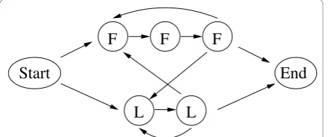
As first case, we consider the well-known example of the dishonest casino [13], see Figure 1. This casino con-sists of a fair (state F) and a loaded dice (state L). The fair dice generates numbers from = {1, 2, 3, 4, 5, 6} with equal probability, whereas the loaded dice generates the same numbers in a biased way. The prop-erties of the dishonest casino are readily captured in a four-state HMM with 8 transition and 12 emission probabilities, six each for each non-silent state FandL. Parameterizing the emission and transition probabilities of this HMM results in two independent transition probabilities and 10 independent emission probabilities, i.e. altogether 12 values to be trained. In order to avoid premature termination of parameter training, we use pseudo-counts of 1 for every parameter to be trained.
The data set for this model consists of 300 sequences of 5000 bp length each. The results of the training experiments are shown in Figures 2 and 3.
Example 2: The extended dishonest casino
In order to investigate a HMM with a more complicated regular grammar, we extended the above example of the
dishonest casino so it can now use the loaded dice (state L) only in multiples of two and the fair dice (state F) only in multiples of three, see Figure 4.
This extended HMM has seven states, the silent Start and End states, two F states and three L states, 11 tran-sition probabilities and 30 emission probabilities. Para-meterizing the HMM’s probabilities yields two independent transition probabilities and 10 independent
F
L
Start
End
Figure 1HMM of the dishonest casino. Symbolic representation of the HMM of the dishonest casino. States are shown as circles, transitions are shown as directed arrows. Please refer to the text for more details.
number of iterations
per
for
mance
0 15 30 45 60 75 90 105 120 135 150
0.0
0.2
0.4
0.6
0.8
1.0
Baum−Welch
Stochastic EM 1 Stochastic EM 3 Stochastic EM 5 Viterbi
emission probabilities to be trained, i.e. 12 parameter values. In order to avoid premature termination of para-meter training, we use pseudo-counts of 1 for every parameter to be trained.
The data set for this model consists of 300 sequences of 5000 bp length each. The results for this extended model are shown in Figures 5 and 6.
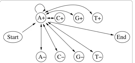
Example 3: The CpG island model
In order to study the features for the different training algorithms for a bioinformatics application, we also investigate an HMM that can be used to detect CpG islands in sequences of genomic DNA [13], see Figure 7. The model consists of 10 states, the silent Start and End states, four non-silent states to model regions inside CpG islands (states A+, C+, G+ and T+) and four non-silent states to model regions outside CpG islands (states A−, C −, G−and T−). The emission probabilities for each of the
eight non-silent states is a delta-function so that any par-ticular state (say A+or A−) has an emission probability of
1 for reading the corresponding DNA nucleotide (in this case A) and a probability of zero for all other nucleotides, i.e.eX+ (Y) =eX−(Y) =δX,YforX,YÎ{A, C, G, T}. This
implies that none of the emission probabilities of this model thus requires training. With a total of 80 transi-tion probabilities the model is, however, highly con-nected as any non-silent state is concon-nected in both directions to any other non-silent state. Parameterizing Figure 3Parameter convergence for the dishonest casino. Average differences of the trained and known parameter values as function of the number of iterations for each training algorithm. For a given number of iterations, we first calculate the average value of the absolute differences between the trained and known value of each emission parameter (left figure) or transition parameter (right figure) and then take the average over the three experiments from the three-fold cross-evaluation. The error bars correspond to the standard deviation from the three cross-evaluation experiments. The algorithms have the same meaning as in Figure 2. Please refer to the text for more information.
F
Start
F
F
End
L
L
Figure 4 HMM of the extended dishonest casino. Symbolic representation of the HMM of the extended dishonest casino. States are shown as circles, transitions are shown as directed arrows. Please refer to the text for more details.
number of iterations
per
for
mance
0 15 30 45 60 75 90 105 120 135 150
0.0
0.2
0.4
0.6
0.8
1.0
Baum−Welch
Stochastic EM 1 Stochastic EM 3 Stochastic EM 5 Viterbi
these transition probabilities results in 33 parameters, 32 of which were determined in training (the transition probability to go to the End state was fixed). In order to avoid premature termination of parameter training, we use pseudo-counts of 1 for every parameter to be trained. The data set for this model consists of 180 sequences of 5000 bp length each. Figures 8 and 9 show the result-ing performance.
Prediction accuracy and parameter convergence Our primary goal is to investigate how the prediction accu-racy of the different training algorithms varies as func-tion of the number of iterafunc-tions. The predicfunc-tion accuracy or performance is defined as the product of the sensitivity and specificity. Figures 2, 5 and 8 show the prediction accuracy as function of the number of
iterations for all three training methods for the respec-tive model.
Another important goal of parameter training is to recover the original parameter values of the correspond-ing model. We therefore also investigate how well the trained parameter values converge to the original para-meter values, see Figures 3, 6 and 9 show the average differences between the trained and known parameter Figure 6Parameter convergence for the extended dishonest casino. Average differences of the trained and known parameter values as function of the number of iterations for each training algorithm. For a given number of iterations, we first calculate the average value of the absolute differences between the trained and known value of each emission parameter (left figure) or transition parameter (right figure) and then take the average over the three evaluation experiments. The error bars correspond to the standard deviation from the three cross-evaluation experiments. The algorithms have the same meaning as in Figure 5. Please refer to the text for more information.
G+ T+
Start
C+ A+
A− C− G− T−
End
Figure 7CpG island HMM. Symbolic representation of the CpG island HMM. States are shown as circles, transitions are shown as directed arrows. Every non-silent state can be reached from the Startstate and has a transition to theEndstate. In addition, every non-silent state is connected in both directions to all non-silent states. For clarity, we here only show the transitions from the perspective of the A+state. Please refer to the text for more details.
number of iterations
per
for
mance
0 15 30 45 60 75 90 105 120 135 150
0.0
0.2
0.4
0.6
0.8
1.0
Baum−Welch
Stochastic EM 1 Stochastic EM 3 Stochastic EM 5 Viterbi
values as function of the number of iterations for each training algorithm and the respective model. Every data point is calculated by first determining the average value of the absolute differences between the trained and known value of each emission parameter (left figures) or transition parameter (right figures) and then taking the average over the three experiments from the three-fold cross-evaluation.
For the dishonest casino and the extended dishonest casino, stochastic EM training performs best, both in terms of performance and parameter convergence. It is interesting to note that the results for sampling one, three or five state paths per training sequence and per iteration are essentially the same within error bars. For these two models, Viterbi training converges fastest, i.e. the Viterbi paths remain the same from one iteration to the next, but the point of convergence is sub-optimal in terms of performance and in particular in terms of para-meter convergence. Baum-Welch training does better than Viterbi training for these two models, but not as well as stochastic BM training as it requires more itera-tions to reach a lower prediction accuracy and worse parameter convergence and as it exhibits the largest var-iation with respect to the three cross-evaluation experi-ments. The latter is due to many high-scoring, sub-optimal state paths. For the CpG island model, all train-ing algorithms do almost equally well, with Viterbi training converging fastest. Table 2 summarizes the CPU time per iteration for the different training
algorithms and models. For all three models, stochastic EM training is faster than Baum-Welch training for one, three or five sampled state paths per training sequence. Viterbi training is even a bit more time efficient than stochastic EM training when sampling one state path per training sequence.
Based on the results from these three small example models, we would thus recommend using stochastic EM training for parameter training.
Conclusion and discussion
A wide range of bioinformatics applications are based on hidden Markov models. Having computationally effi-cient algorithms for training the free parameters of these models is key to optimizing the performance of these models and to adapting the models to new data sets, e.g. biological data sets from a different organism.
We here introduce two new algorithms which render the memory requirements for Viterbi training and sto-chastic EM training independent of the sequence length. This is achieved by replacing the usual bi-directional two-step procedure (which involves first calculating the Viterbi matrix and then retrieving the Viterbi path (in case of Viterbi training) or first calculating the forward matrix and the backward matrix before estimating counts (in case of Baum-Welch training)) by a one-step proce-dure which scans each training sequence only in a one-directional way. For an HMM withM states and a con-nectivity ofTmax, a training sequence of lengthLand one
iteration, our new algorithm reduces the memory requirement of Viterbi training from (ML) to (M ) while keeping the time requirement of (MTmaxL)
unchanged, see Table 1 for details. For stochastic EM training where Kis the number of state paths sampled for every training sequence in every iteration, the mem-ory requirements are (as, typically, L ≫ K + 1 ≥ K+
Tmax/M ) reduced from (ML) to (MK + Tmax) while
the time requirement per iteration changes from
number of iterations
tpro
b con
vergence
0 15 30 45 60 75 90 105 120 135 150
0.0
0.1
0.2
0.3
0.4
0.5
Baum−Welch
Stochastic EM 1 Stochastic EM 3 Stochastic EM 5 Viterbi
Figure 9Parameter convergence for the CpG island model. Average differences of the trained and known parameter values as function of the number of iterations for each training algorithm. For a given number of iterations, we first calculate the average value of the absolute differences between the trained and known value of each transition parameter (this model does not have any emission parameters that require training) and then take the average over the three cross-evaluation experiments. The error bars correspond to the standard deviation from the three cross-evaluation experiments. The algorithms have the same meaning as in Figure 8. Please refer to the text for more information.
Table 2 CPU time use for different models
CPU time (sec) per iteration
dishonest extended dishonest
CpG island Casino Casino Model
Baum-Welch training 8.85 5.94 22.22 stochastic EM trainingK= 1 5.12 3.42 5.42 stochastic EM trainingK= 3 6.02 4.42 10.30 stochastic EM trainingK= 5 7.06 5.38 14.84
Viterbi training 4.42 2.84 5.00
(TmaxL(M + K)) to (TmaxLMK) depending on the
user-chosen value ofK. An added advantage of our two new algorithms is they are easier to implement than the corre-sponding default algorithms for Viterbi training and sto-chastic EM training. In addition to introducing the two new algorithms for Viterbi training and stochastic EM training, we also examine their practical merits for three small example models by comparing them to the linear-memory algorithm for Baum-Welch training which was introduced earlier. Based on our results from these three (non-representative) models, we would recommend using stochastic EM training for parameter training.
We have implemented the new algorithms for Viterbi training and stochastic EM training as well as the lin-ear-memory algorithm for Baum-Welch training into our HMM-compiler HMMCONVERTER[37] which can be used to set up a variety of HMM-based applications and which is freely available under the GNU General Pub-lic License version 3 (GPLv3). Please see http://people.cs. ubc.ca/~irmtraud/training for more information and the source code.
We hope that the new parameter training algorithms introduced here will make parameter training for HMM-based applications easier, in particular those in bioinformatics.
Acknowledgements
Both authors would like to thank the anonymous referees for providing useful comments. We would also like to thank Anne Condon for giving us helpful feedback on our manuscript. Both authors gratefully acknowledge support by a Discovery Grant of the Natural Sciences and Engineering Research Council, Canada, and by a Leaders Opportunity Fund of the Canada Foundation for Innovation to I.M.M.
Authors’contributions
TYL and IMM devised the new algorithms, TYL implemented them, TYL and IMM conducted the experiments, evaluated the experiments and wrote the manuscript. All authors read and approved the final manuscript.
Competing interests
The authors declare that they have no competing interests.
Received: 21 June 2010 Accepted: 9 December 2010 Published: 9 December 2010
References
1. Meyer I, Durbin R:Gene structure conservation aids similarity based gene prediction.Nucleic Acids Research2004,32(2):776-783.
2. Stanke M, Keller O, Gunduz I, Hayes A, Waack S, Morgenstern B:
AUGUSTUS: ab initio prediction of alternative transcripts.Nucleic Acids Research2006,34:W435-W439.
3. Won K, Sandelin A, Marstrand T, Krogh A:Modeling promoter grammars with evolving hidden Markov models.Bioinformatics2008,
24(15):1669-1675.
4. Finn R, Tate J, Mistry J, Coggill P, Sammut S, Hotz H, Ceric G, Forslund K, Eddy S, Sonnhammer E, Bateman A:The Pfam protein families database.
Nucleic Acids Research2008,36:281-288.
5. Nguyen C, Gardiner K, Cios K:A hidden Markov model for predicting protein interfaces.Journal of Bioinformatics and Computational Biology 2007,5(3):739-753.
6. Krogh A, Larsson B, von Heijne G, Sonnhammer E:Predicting transmembrane protein topology with a hidden Markov model: application to complete genomes.Journal of Molecular Biology2001,
305(3):567-580.
7. Bjöorkholm P, Daniluk P, Kryshtafovych A, Fidelis K, Andersson R, Hvidsten T:
Using multi-data hidden Markov models trained on local neighborhoods of protein structure to predict residue-residue contacts.Bioinformatics 2009,25(10):1264-1270.
8. Qian X, Sze S, Yoon B:Querying pathways in protein interaction networks based on hidden Markov models.Journal of Computational Biology2009,
16(2):145-157.
9. Drawid A, Gupta N, Nagaraj V, Gélinas C, Sengupta A:OHMM: a Hidden Markov Model accurately predicting the occupancy of a transcription factor with a self-overlapping binding motif.BMC Bioinformatics2009,
10:208.
10. king F, Sterne J, Smith G, Green P:Inference from genome-wide association studies using a novel Markov model.Genetic Epidemiology 2008,32(6):497-504.
11. Su S, Balding D, Coin L:Disease association tests by inferring ancestral haplotypes using a hidden markov model.Bioinformatics2008,
24(7):972-978.
12. Juang B, Rabiner L:A segmental k-means algorithm for estimating parameters of hidden Markov models.IEEE Transactions on Acoustics, Speech, and Signal Processing1990,38(9):1639-1641.
13. Durbin R, Eddy S, Krogh A, Mitchison G:Biological sequence analysis: Probabilistic models of proteins and nucleic acidsCambridge: Cambridge University Press; 1998.
14. Besemer J, Lomsazde A, Borodovsky M:GeneMarkS: a self-training method for prediction of gene starts in microbial genomes. Implications for finding sequence motifs in regulatory regions.Nucleic Acids Research 2001,29(12):2607-2618.
15. Lunter G:HMMoC–a compiler for hidden Markov models.Bioinformatics 2007,23(18):2485-2487.
16. Ter-Hovhannisyan V, Lomsadze A, Cherno Y, Borodovsky M:Gene prediction in novel fungal genomes using an ab initio algorithm with unsupervised training.Genome Research2008,18:1979-1990.
17. Viterbi A:Error bounds for convolutional codes and an assymptotically optimum decoding algorithm.IEEE Trans Infor Theor1967, 260-269. 18. Keibler E, Arumugam M, Brent MR:The Treeterbi and Parallel Treeterbi
algorithms: efficient, optimal decoding for ordinary, generalized and pair HMMs.Bioinformatics2007,23(5):545-554.
19. Sramek R, Brejova B, Vinar T:On-line Viterbi algorithm for analysis of long biological sequences.Algorithms in Bioinformatics, Lecture Notes in Bioinformatics2007,4645:240-251.
20. Lifshits Y, Mozes S, Weimann O, Ziv-Ukelson M:Speeding Up HMM Decoding and Training by Exploiting Sequence Repetitions.Algorithmica 2009,54(3):379-399.
21. Baum L:An equality and associated maximization technique in statistical estimation for probabilistic functions of Markov processes.Inequalities 1972,3:1-8.
22. Dempster A, Laird N, Rubin D:Maximum likelihood from incomplete data via the EM algorithm.J Roy Stat Soc B1977,39:1-38.
23. Larsen T, Krogh A:EasyGene - a prokaryotic gene finder that ranks ORFs by statistical significance.BMC Bioinformatics2003,4:21.
24. Jensen JL:A Note on the Linear Memory Baum-Welch Algorithm.Journal of Computational Biology2009,16(9):1209-1210.
25. Khreich W, Granger E, Miri A, Sabourin R:On the memory complexity of the forward-backward algorithm.Pattern Recognition Letters2010,
31(2):91-99.
26. Elliott RJ, Aggoun L, Moon JB:Hidden Markov Models. Estimation and ControlBerlin, Germany: Springer-Verlag; 1995.
27. Sivaprakasam S, Shanmugan SK:A forward-only recursion based hmm for modeling burst errors in digital channels.IEEE Global Telecommunications Conference1995,2:1054-1058.
28. Turin W:Unidirectional and parallel Baum-Welch algorithms.IEEE Trans Speech Audio Process1998, ,6:516-523.
29. Miklós I, Meyer I:A linear memory algorithm for Baum-Welch training.
BMC Bioinformatics2005,6:231.