Modelling and Visualization of Three Dimensional Objects Using Inexpensive Digital Cameras

Modelling and Visualization of Three Dimensional Objects

Using Inexpensive Digital Cameras

Ismail Elkhrachy

College of Engineering, Civil Engineering Department, Najran University, K.S.A, king abdulaziz Rd., 11001, P.O. Box 1988,

Najran, Saudi Arabia

Faculty of Engineering Civil Department, Al-Azhar University, Nasr City, 11371 Cairo, Egypt

Emai: [email protected]

ABSTRACT

This paper analyses and evaluate the precision and the accuracy the capability of low-cost terrestrial photogrammetry by using many digital cameras to construct a 3D model of an object. To obtain the goal, a building façade has imaged by two inexpensive digital cameras such as Canon and Pentax camera. Bundle adjustment and image processing calculated by using Agisoft PhotScan software. Several factors will be included during this study, different cameras, and control points. Many photogrammetric point clouds will be generated. Their accuracy will be compared with some natural control points which collected by the laser total station of the same building. The cloud to cloud distance will be computed for different comparison 3D models to investigate different variables. The practical field experiment showed a spatial positioning reported by the investigated technique was between 2-4cm in the 3D coordinates of a façade. This accuracy is optimistic since the captured images were processed without any control points.

Keywords

1.

Introduction

Collecting and modelling 3D surface coordinates data for an object is significant importance in the field of heritage conservation. The precise 3D models of buildings are used for visualization, maintenance, restoration and documentation process. In order to obtain the 3D model, many techniques and methods have been used to collect its surface data, such as scanning by terrestrial laser scanning, topographic, close-range photogrammetry and surveying traditional techniques such as total station instrument [1]. Terrestrial Scanning and photogrammetry are the most common techniques in the last year for many researchers [2]. Photogrammetry is viewed as the best solution for the processing of image data, having the capacity to deliver at any scale of application accurate, metric and detailed 3D surface information [3]. In digital close photogrammetry technique, by using pictures captured with a camera at close range from different angles, the geometric details of any complex shape such as a façade that can be used to create accurate 3D models of objects [5],[9] and [3]. The ability to measure and record surfaces is important to many scientific disciplines and both photogrammetry and laser scanning provide the required capability.

Nowadays digital camera technology is one of the most rapidly developed, cheap, great storage capacity and to use. Their sensor resolution is increasing rapidly, with new ranges of 12 to 30 Mega-pixel. The price of the Canon EOS REBEL T5i its price about 400$. However, you also need photogrammetry software to create a 3D model of the object you have photographed. There are many photogrammetry software’s, some of them are free and the others are commercial. we mainly use the photogrammetric software Agisoft PhotScan Professional Edition costs 3,500$. You need also a tool or equipment to measure data on site to scale, rotate and translate the final model. The laser total station Leica TS 06 Plus is used in our test field. It costs approximately 7,000$ and could be rented from 50$ /day. Thus, the total amount goes from 4,000$ to 11,000$.

On the other hand, using laser scanner techniques is much more expensive than photogrammetry: Leica ScanStation P40 sale price is over 32,500$. Point cloud processing software should be added to these expenses. The Leica Cyclone 3D Point Cloud Processing software costs from 2,000$ to 14,000$, it has different modules. The average renting option is also is 800$/day. The previous cost analysis summarizes why the terrestrial photogrammetry is a low-cost technique to collect 3D surface information.

1.1

Related work

There are also many investigations on digital image-based modelling for complex buildings. Photogrammetry and laser scanning were and compared for accurate modelling of architectural sites by [4]. Many researchers have tried to analyse and investigate many low-cost image based 3D documentation techniques for cultural heritage [5], and [6] Also, a photogrammetric process to achieve the 3-D reconstruction of archaeological sites by using low-cost photogrammetric techniques was presented by [7], also by combining different techniques, mainly topography and photogrammetry, it was possible to obtain dense point clouds of a complex architectonic element [8]. Numerous tests have exhibited that digital none metric cameras are fit for obtaining digital elevation model to sub-millimetre accuracies [9] and [10]. Some practical rules and benefits of the low-cost image for obtaining the 3D model for heritage preservation in Nepal, after 2015 earthquake introduced by [11]. A range of variables that affect the quality of photogrammetric results such as used software, number of photos and control points considered by [12]. A certain digital measuring scheme based on a GPS-enabled digital camera tested by [13]. Many free software are used in low-cost image reconstruction on sites tested by [14]. Their results demonstrated that software makes a difference and the results are not constantly steady.

1.2

Paper objectives

total station. The normal distribution of residuals will be tested. The prober outliers technique will be defined for the data filtering process.

2.

Study area description and data acquisition

An experiment has been conducted aiming to archive the paper objectives. The test building was the façade of the college of engineering, Najran University, south of the Kingdom of Saudi Arabia (KSA). The façade dataset covers a large area: 40 m in width and up to 35 m in height. The data acquisition took place on March 03, 2018. It has low ornate features, so detailed images from the ground is not a challenge. Two types from low-cost none metric digital camera has been selected for investigation. Table 1 shows used cameras and their sensor parameters.

Table 1 Used digital camera parameters

Sensor Image size Focal length (mm)

Number of

used images ISO Canon EOS REBEL

T5i 2592x1728 18 8 100

Pentax Optio E50 3264x2448 6.2 8 100

2.1

Taking pictures

For every tested camera, many exposures from different stations were taken. The camera was fixed by hand, not on a tripod, and the camera settings for every exposure were (within the limits of the camera used; maximum f-stop, minimal ISO to reduce any noise and fixed focus. Some unusable images such as; blurred images, limited area covered etc.) were discarded from the original set of images. From the remaining photographs, two sets of images were created. Final used images for canon and Pentax was 8 photos. Manually selecting photos allows reducing the number of images, avoiding redundancy and speeding-up the software during the processing step. Image selection step may appear tedious, but it may significantly reduce the processing time and the control points (CPs) tagging step.

2.2

Reference data

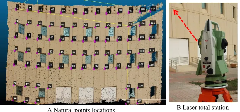
A Natural points locations B Laser total station

Figure 1 Imaged facade and natural targets used as CPs.

In this case, instead of using coded target, we used “natural targets” (any natural mark on the building façade i.e. corners of windows, intersections, and doors,) to not damage the building. The chosen points must not be mistakenly, so those can be carefully chosen to be visible in the photographs and superbly recognizable. The coordinates of 116 well spread natural marks used as CPs measured from 2 stations using Leica TS 06 Plus laser total station. The mean value of the 3D positional difference for CPs obtained from two epochs was 4mm. Some of the CPs were used during the bundle adjustment and accuracy assessment of obtained 3D models.

3.

Methodology

3.1

From images to point clouds

A point cloud is a set of points in a 3D coordinate system and represents the external surface of an object. From a set of images and algorithms, it is possible to derive metric and accurate 3D information of the scene. The workflow consists of a camera calibration, images orientation, and a point cloud generation. After that, the 3D measurements, modelling, texture mapping, and visualization can be done. Nowadays there are several commercial software could be used to get a 3D model of captured images such as Photomodeler, Agisoft PhotScan, iWitness, MicMac, 3DF Zephir, etc. They are mainly produced by the computer vision developers. Many researchers recommended and used Agisoft PhotScan, therefore it will be used during this work to get different 3D models. Our investigation will firstly involve making a range of 3D reconstructions of the taken photographs. These will be varied in terms of their input images and control points.

3.1.1 Bundle adjustment

equations are the formula used as a mathematical model to adjust these bundles. The first known method for bundle adjustment was in 1958 and was used to minimize the projection error after estimating point coordinates and camera positions from aerial images using least squares [15]. The image processing was performed using PhotoScan Professional. It is a commercial product developed by Agisoft PhotScan® for digital photogrammetry, commonly used for archaeological and mapping purposes.

In this work, two different BA solution are investigated to test the efficiency of the used digital camera. The first solution of BA is performed with best CPs to get the most accurate 3D model. The second is performed without any CPs. For scaling the uncontrolled models, two scale bars measurement were made with a long tape, one to scale the model and the second to check the result.

3.1.1 Ground Control points

To provide the transformation between images and object space frame, the additional measurements are needed to add the scale, position, and orientation of the model in the required coordinate system. The transformation is usually ensured by using some CPs, whose coordinates are known in the image as well as in the object frame. They also should improve the results by used software. The position of CPs can be surveyed by the laser total station. Another way is to leave the model in a free-network mode and to retrieve the correct scale using a known distance on the object. Therefore 3D models from the same photoset will be made with and without CPs to test whether this is valid, and to what degree of accuracy can be obtained. Also, the total number of CPs used has a significant effect. Models will be created from total CPs (21 points) and reduced them to be only 4 points, to see if there is any change in the results. The four control point scenarios are displayed in Figure 2.

Figure 2 Configurations of the 4, ,8, 12 and 21 control points, clockwise from top-left.

3.2

Accuracy measures and data comparison

3.2.1 Cloud-to-cloud compare (signed distance computation)

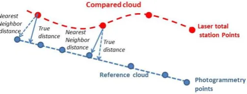
source software such as CloudCompare and Meshlab [16] and [17]. For each comparison, direct cloud-to-cloud (C2C) distance are computed between each photogrammetric point cloud and the reference one. C2C is a direct 3D comparison of the point clouds, without any need to create regular grids or meshes of the original data or to compute the normal to the surfaces. Distance calculations are based on different performing algorithms, such as the Nearest neighbour, Nearest neighbour with local modelling Normal shooting and Iterative Closest Point (ICP). Each point of the former and finding its nearest neighbour on the latter [18] and [19].

The default way to compute C2C is the nearest neighbour distance (as shown in Figure 3) because of its simplicity. For each point of the compared cloud, CloudCompare searches the nearest point in the reference cloud and computes their (Euclidean) distance. Its results can be unreliable due to roughness and different point density between compared clouds.

Figure 3 Cloud-to-cloud distance based on nearest neighbor.

The 3D-virtual reconstruction accuracy has been assessed through CPs (ground control points) comparing the XYZ coordinates of the points measured on the “real model” with laser total station and the other ones supplied by the photogrammetric reconstruction on the “virtual model” for the homologous points.

3.2.2 Statistical analysis

Accuracy measures are derived from coordinate differences of some points obtained from photogrammetric solution and another reference one. The reference values should be another method which can produce reference values with an accuracy which at least 3 times higher [20] and [21]. Such points which can be determined in both systems are named checkpoints or control points. These differences are called ‘discrepancies or errors’ as shown in Equation (1) and (2).

Ex= (xpho− xtot), Ey = (ypho− ytot), Ez = (zpho− ztot) (1)

𝐷 = √(Ex)2+ (Ey)2+ (E𝑧)2 (2)

Where:

Ex, Ey, Ez = Errors or residuals in x, y and z directions.

xpho, ypho, zpho = estimated coordinates from image measurements

D = error length based on coordinate residuals

From the differences the Root Mean Square Error (RMSE), the Mean value and the Standard Deviation (σ) are calculated by using Equations (3), (4) and (5).

RMSEx= √ ∑(E_x)2

n , RMSEy= √ ∑(E_y)2

n , RMSEz= √ ∑(E_z)2

n (3)

𝑅𝑀𝑆𝐸total= √(𝑅𝑀𝑆𝐸𝑥)2+ (𝑅𝑀𝑆𝐸𝑦)2+ (𝑅𝑀𝑆𝐸𝑧)2 (4)

σ = √∑(x − x)

2

n − 1 (5)

Where:

RMSEx, RMSEy, RMSEz = root mean square error for X, Y, Z coordinates

𝑅𝑀𝑆𝐸total = total root mean square error for a point

n = number of observations in the sample.

x = the observed values of the sample items

x = is the mean value of these observations

σ = the sample standard deviation

After calculating the errors, a histogram of the errors will inform whether the distribution of the errors is normal or not. The curve for a normal distribution can be superimposed. If the curve does not match the data very well, then the distribution is not normal. A better diagnostic plot in order to detect a deviation from the normal distribution is the so-called quantile-quantile (Q-Q) plot. Also, the Skewness value gives an indication of departure from symmetry in a distribution and is expressed as:

𝑆𝑘𝑒𝑤𝑛𝑒𝑠𝑠 =∑ (𝑥𝑖− 𝜇)

3 𝑛

𝑖=1

(𝑛 − 1)𝜎3 (6)

The skewness for a normal distribution is zero, and any symmetric data should have a skewness near zero. Negative values for the skewness indicate data that are skewed left and positive values for the skewnessindicate data that are skewed right. The Kurtosis is a measure of the data are peaked or flat relative to a normal distribution and is expressed as:

𝐾𝑢𝑟𝑡𝑜𝑠𝑖𝑠 =∑ (𝑥𝑖− 𝜇)

4 𝑛

𝑖=1

(𝑛 − 1)𝜎4 (7)

If the distribution is perfectly normal, Skewness and Kurtosis values of zero and three are obtained, respectively.

BA a technique is based on the idea that many light rays which come from the camera are forming a bundle of rays all intersect to generate 3D positions. Collinearity equations are the formula used as a mathematical model to adjust these bundles. The first known method for bundle adjustment was in 1958 and was used to minimize the projection error after estimating point coordinates and camera positions from aerial images using least squares [22]. The image processing was performed using PhotoScan Professional. It is a commercial product developed by Agisoft® for digital photogrammetry, commonly used for archaeological and mapping purposes. Agisoft PhotScan software used to reconstruct 3D models. To get the photogrammetry solution using this software, four main stages should be done [23] :

9 2. Figure4).

3. Creation of the dense point cloud using the estimated camera positions and the pictures themselves. The software calculates depth maps for each image.

4. Reconstruction of a 3D polygonal mesh representing the object surface based on the dense point cloud.

5. The reconstructed mesh can be textured following different mapping modes.

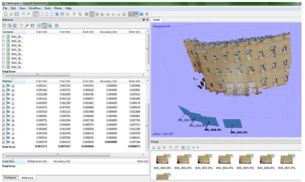
Figure 4 Agisoft PhotScan parameters

All the mentioned steps are fully automated. Figure 5 shows a dense point cloud as an example of obtained data. The software is user-friendly, but the adjustment of parameters is limited by pre-defined values. It can be noted that the user manual describes mainly the general workflow and gives only very limited details regarding the theoretical basis of the underlying calculations and the associated parameters.

Figure 5 Dense point cloud detail after 3D model reconstruction.

4.1

Comparison of The bundle Block Adjustment for different

cameras

10

4.1.1 BA accuracy based on using CPs

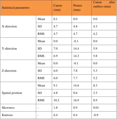
After georeferencing using 38 CPs the accuracies are listed in Table 2.

Table 2 Statistical of discrepancies after georefrencing using 38 CPs.

Statistical parameters Canon

(mm)

Pentax (mm)

Canon after outliers (mm)

X-direction

Mean 0.1 0.0 0.0

SD 4.7 4.8 4.3

RMS 4.7 4.7 4.2

Y-direction

Mean 0.0 -0.1 0.0

SD 7.0 14.4 5.9

RMS 6.9 14.3 5.8

Z-direction

Mean 0.0 -0.1 0.0

SD 6.0 7.8 5.3

RMS 6.0 7.7 5.2

Spatial position

Mean 9.1 14.6 8.3

SD 4.8 8.6 3.3

RMS 10.2 16.9 8.9

Skewness - 1.8 0.9 0.01

Kurtosis - 6.4 0.4 -0.9

11

Figure 6 Residuals histogram and Q-Q plot for Canon before outliers.

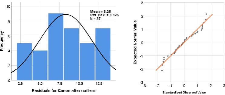
The histograms show that the tails of the residuals distribution are small “thin” or “skinny” compared with the normal distribution while that data has positively skewed.

After the

filtering, the resulting datasets are more close to a normal distribution

: this is confirmed by both graphical

analyses (Q-Q plot in

Figure 7) and

Kurtosis and Skewness

parameters in Table 2

Figure 7 Residuals histogram and Q-Q plot for Canon after outliers.

12

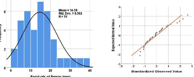
Figure 8 Residuals histogram and Q-Q plot for Pentax camera.

The obtained 3D model accuracies by using two low-cost digital cameras an expected improvement in the position accuracy of the computed coordinates, related to the precision of used laser total station observations. Analysing the obtained results gives attractive finding; since the position accurses between 1-1.7cm were achieved using two low-cost digital cameras.

4.1.2 Cloud to cloud comparisons

Many researchers have used the terrestrial laser scanner as a reference surface to compare the accuracy of the obtained 3D model for other techniques such as photogrammetry or even Mobil mapping system (MMS). For our case the terrestrial laser scanner data aren’t available, therefore 116 natural CPs which are collected by laser total station are used as reference points instead of laser scanner data. CloudCompare software has the ability to calculate cloud to cloud distances (C2C) between two cloud points and represents the differences graphically to show which areas match the reference cloud data closely and which do not. Before calculation, t

he

bottom part is removed from the investigation

due to the presence of obstructions, such

as

, etc.

Table 3 Statistical results of the C2C absolute distances between the model from Canon and two other cameras.

Reference Compared Mean

(mm)

Standard deviation (mm)

RMSE (mm)

116 CPs from laser total station

Canon 16 26 31

Pentax 21 67 71

13

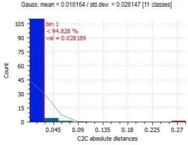
however, Pentax has 98% of differences less 7cm as shown in Figure 9. Results clearly indicate that different digital cameras significantly affect the quality of results.

Canon

Pentax

Figure 9 Histograms of C2C absolute distances testing of models generated from Canon and Pentax cameras compared to 116 laser total station points.

4.2

Relative comparison between Canon and Pentax models

The relative precision between obtained two 3D models is presented. While the Canon camera gave an accuracy 1cm, therefore the canon model will be used as the reference surface to compute the comparison. Obtained 3D models from two cameras are compared by each other. The C2C distances were calculated. The Canon model is used as reference surface and the model from Pentax is compared. The mean value and stander deviation of distances were 2.7cm and 4.3cm. The RMSE was 5.2cm (Table 4).

Table 4 C2C absolute distances for Relative comparison

Reference Compared Mean

(mm)

Standard deviation (mm)

RMSE (mm)

14

Figure 10 demonstrates a graphical representation of C2C distances between the compared two surfaces. The area with red colour at windows and boundaries has a difference more than 8cm. Blue means the differences values less than 2cm, green means difference less than 4cm).

Figure 10 C2C absolute distances for Relative comparison between Canon and Pentax models

Also Figure 11 shows the histograms of obtained results, 95% of points are less than 7.7cm while 54% are less than 1.6cm.

Figure 11 Histograms of C2C absolute distances for Pentax using Canon as reference model. 53.8% of points < 1.6cm and 94.24% are <7.6cm.

4.3

BA accuracy

without using

control points

15

are still aligned by ICP to keep the test consistent. This rotates and translates it to best fit the models obtained by using CPs clouds, without changing the scale. Outlying points are excluded from the process in order to improve the fit. The obtained statistical results of the C2C absolute distances without using CPs are listed in Table 5

Table 5 Statistical results of the C2C absolute distances without using CPs

Compared Reference Mean

(mm)

Standard deviation (mm)

RMSE (mm)

116 CPs from laser total station

Canon 23 13 26

Pentax 41 121 26

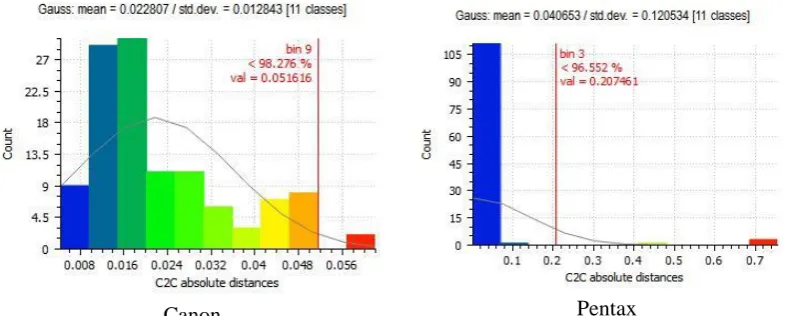
The mean value of C2C distances was 23mm and 41mm for Canon and Pentax camera respectively. The obtained standard deviations were 13cm and 121cm. This concludes that obtained 3D model from Pentax was noisy while its standard deviation was 121mm. Also, 98% of obtained point cloud within 5cm for Canon, while at97% of point cloud are less than 21cm (Figure 12).

Canon Pentax

Figure 12 Histograms of C2C absolute distances for Canon and Pentax without using any CPs. Laser total station as reference model

4.4

Effect of the number of control points on the results

16 Table 6 Number of CPs effect.

CPs number

Canon Pentax

Mean (mm)

SD (mm)

RMS (mm)

Mean (mm)

SD (mm)

RMS (mm)

0 23.0 13.0 26.0 41.0 121.0 26.0

4 16.0 20.0 26.0 25.0 60.0 65.0

8 16.0 25.0 30.0 32.0 76.0 82.0

12 14.0 20.0 24.0 30.0 76.0 81.0

21 14.0 21.0 25.0 21.0 76.0 79.0

38 16.0 26.0 31.0 21.0 67.0 71.0

The mean distances were stable between 4 and 38 control points for Canon camera was only 15mm. Without control points the difference is 7mm.

Figure 13 Mean values of C2C distances for different CPs.

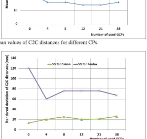
Figure 14 Standard deviation values of C2C distances for different GPs.

17

5.

Discussion

The most accurate results were obtained by using control points, the mean values of C2C distances were between 16mm and 21mm. The lowest mean C2C distance was 14mm, achieved by the canon camera when 14 control points are used. By using 8 control points the accuracy are stable and has very small change. This mean values of C2C distances using 8 control points good distributed are the optimum number of control points for both used digital cameras. In case of no control points are used, the mean value of C2C distances was between 23-41mm. Comparisons indicate that the largest variances between the laser total station and the photogrammetric outcomes can be seen in the case of a low-cost Pentax camera. C2C distances between laser total station data and photogrammetry outcomes when using Canon digital camera are distinctly lower. The mean value of the differences is 14mm. When a larger number of CPs is employed, the risk of the model deformation rises as shown in Figure 14. This risk can be reduced by using a larger number of CPs. After using more than 12 CPs the standard deviation starts to increase. The corresponding error distribution (Figure 10) demonstrates that the areas conveying the biggest C2C distances at zones imaged from high distances and with high acquisition angles, such as the right and upper parts of the façade.

Furthermore

the same

error patterns occurred

6.

Conclusions

Low-cost 3D model can be obtained with Agisoft Photoscan software and an inexpensive digital camera such as Canon or Pentax. The obtained accuracy shows that this technique is comparable in many considerations (accuracy, time demands, demanded outputs) and can be applied for a building documentation. It has faster acquisition, low-cost, slower point cloud production process when it compared with the terrestrial laser scanner. Both tested cameras show significant noise level in the data, noise level reaches values as high as several centimetres for Canon camera. For high accuracy purposes, the user should be aware to get the right digital sensor. In case of high accuracy documentation, control points should be used and distributed appropriately.

Although there were few control points acquired by laser total station used in the

comparison process, when they compared with the huge point cloud from

terrestrial

laser scanner, they gave the same accuracy results during test field.

distances are measured in

the other direction, from the laser

to the photogrammetric clouds.

complete dense, but

he control

are not dense then the C2C

distances will be large and

mean

standard deviation will be higher.

Acknowledgements:

18

7.

References

1.

Scherer, M.,

About the synthesis of different methods in surveying.

INTERNATIONAL ARCHIVES OF PHOTOGRAMMETRY REMOTE

SENSING AND SPATIAL INFORMATION SCIENCES, 2002.

34(5/C7): p.

423-429.

2.

Remondino, F.,

Heritage recording and 3D modeling with photogrammetry and

3D scanning.

Remote Sensing, 2011. 3(6): p. 1104-1138.

3.

Luhmann, T., et al.,

Close range photogrammetry: principles, techniques and

applications

. 2006: Whittles.

4.

Barsantia, S.G., F. Remondino, and D. Visintini,

3D surveying and modelling

of archaeological sites-some critical issues.

ISPRS photogrammetry, remote

sensing and spatial information sciences, Strasbourg, France, Sept, 2013: p.

2-6.

5.

Boochs, F., et al.

Low-cost image based system for nontechnical experts in

cultural heritage documentation and analysis

. in

Proc. of XXI International

CIPA Symposium

. 2007.

6.

Remondino, F. and A. Rizzi,

Reality-based 3D documentation of natural and

cultural heritage sites—techniques, problems, and examples.

Applied

Geomatics, 2010. 2(3): p. 85-100.

7.

Barazzetti, L., et al.,

Photogrammetric survey of complex geometries with

low-cost software: Application to the ‘G1′ temple in Myson, Vietnam.

Journal of

Cultural Heritage, 2011. 12(3): p. 253-262.

8.

Robleda Prieto, G. and A. Pérez Ramos,

MODELING AND ACCURACY

ASSESSMENT FOR 3D-VIRTUAL RECONSTRUCTION IN CULTURAL

HERITAGE USING LOW-COST PHOTOGRAMMETRY: SURVEYING OF

THE “SANTA MARÍA AZOGUE” CHURCH’S FRONT.

3D-ARCH 2015 “3D

virtual reconstruction and visualization of complex architecture, 2015: p.

263-270.

9.

Chandler, J.H., J.G. Fryer, and A. Jack,

Metric capabilities of low‐cost digital

cameras for close range surface measurement.

The Photogrammetric Record,

2005. 20(109): p. 12-26.

10.

Läbe, T. and W. Förstner.

Geometric stability of low-cost digital consumer

cameras

. in

Proceedings of the 20th ISPRS Congress, Istanbul, Turkey

. 2004.

11.

Dhonju, H., et al.,

Feasibility study of low-cost image-based heritage

documentation in Nepal.

The International Archives of Photogrammetry,

Remote Sensing and Spatial Information Sciences, 2017. 42: p. 237.

12.

Altman, S., W. Xiao, and B. Grayson,

EVALUATION OF LOW-COST

TERRESTRIAL PHOTOGRAMMETRY FOR 3D RECONSTRUCTION OF

COMPLEX BUILDINGS.

ISPRS Annals of Photogrammetry, Remote Sensing

& Spatial Information Sciences, 2017. 4.

13.

Ragab, A.F. and A.E. Ragheb,

Efficiency Evaluation of Processed

Photogrammetric Data Captured by GPS Digital Camera.

World Applied

Sciences Journal, 2010. 8(4): p. 414-421.

14.

Remondino, F., et al.

Low-cost and open-source solutions for automated image

orientation–A critical overview

. in

Euro-Mediterranean Conference

. 2012.

Springer.

15.

Brown, D.C.,

A solution to the general problem of multiple station analytical

stereotriangulation

. 1958: D. Brown Associates, Incorporated.

16.

Cignoni, P., et al.

Meshlab: an open-source mesh processing tool

. in

19

17.

Girardeau-Montaut, D.,

Cloudcompare-open source project.

OpenSource

Project, 2011.

18.

Koutsoudis, A., et al.,

Multi-image 3D reconstruction data evaluation.

Journal

of Cultural Heritage, 2014. 15(1): p. 73-79.

19.

Lague, D., N. Brodu, and J. Leroux,

Accurate 3D comparison of complex

topography with terrestrial laser scanner: Application to the Rangitikei canyon

(NZ).

ISPRS journal of photogrammetry and remote sensing, 2013. 82: p.

10-26.

20.

Gesch, D., et al.,

The national elevation dataset.

Photogrammetric engineering

and remote sensing, 2002. 68(1): p. 5-32.

21.

Photogrammetry, A.S.f. and R. Sensing,

ASPRS accuracy standards for

large-scale maps.

Photogrammetric Engineering and Remote Sensing, 1990. 56(7): p.

1068-1070.

22.

Abdel-Aziz, Y., H. Karara, and M. Hauck,

Direct linear transformation from

comparator coordinates into object space coordinates in close-range

photogrammetry.

Photogrammetric Engineering & Remote Sensing, 2015.

81(2): p. 103-107.

23.

Jaud, M., et al.,

Assessing the accuracy of high resolution digital surface models

computed by PhotoScan® and MicMac® in sub-optimal survey conditions.

Remote Sensing, 2016. 8(6): p. 465.