http://www.sciencepublishinggroup.com/j/ajmcm doi: 10.11648/j.ajmcm.20190402.12
ISSN: 2578-8272 (Print); ISSN: 2578-8280 (Online)
Application of Multiple Linear Regression Technique to
Predict Noise Pollution Levels and Their Spatial Patterns in
the Tarkwa Mining Community of Ghana
Peter Ekow Baffoe
1, *, Alfred Allen Duker
21
Department of Geomatic Engineering, Faculty of Mineral Resources Technology, University of Mines and Technology, Tarkwa, Ghana 2
Department of Geomatic Engineering, School of Engineering, Kwame Nkrumah University of Science and Technology, Kumasi, Ghana
Email address:
*
Corresponding author
To cite this article:
Peter Ekow Baffoe, Alfred Allen Duker. Application of Multiple Linear Regression Technique to Predict Noise Pollution Levels and Their Spatial Patterns in the Tarkwa Mining Community of Ghana. American Journal of Mathematical and Computer Modelling.
Vol. 4, No. 2, 2019, pp. 36-44. doi: 10.11648/j.ajmcm.20190402.12
Received: April 30, 2019; Accepted: June 4, 2019; Published: June 20, 2019
Abstract:
Predicting and preventing intraurban noise levels in our communities are very challenging for urban planning, epidemiological studies and environmental management, especially in the developing world. Most existing noise-predicting models are limited in providing changes in noise levels during intraurban development and the corresponding noise pollution. In this study, noise levels were measured at 50 purpose-designed monitoring stations and then a land-use regression model was developed for the intraurban noise prediction applying the multiple linear regression (MLR) technique. The measured and the predicted noise levels were compared. These were further compared with noise estimates from a standard noise model, Lyons Empirical model. The results from the developed MLR model did not show any significant differences in the patterns as compared with those of the Lyons Empirical model. The model performance indicators showed a standard deviation of 1.585, high correlation (R) of 0.98, R2 of 0.961 and RMSE of 1.569. The resulting maps showed a heterogeneous distribution of the noise pollution levels in the community. This confirms the usefulness of the method for assessing the spatial pattern of noise pollution in a community. This makes it a useful tool for urban planning, epidemiological studies and environmental management.Keywords: Noise Level, Noise Pollution, Noise Models, Land Use Regression Models
1. Introduction
Intraurban noise pollution is prevalent in our cities, especially in the mining communities where many factors contribute to noise pollution and distribution. Increase in urban noise pollution brings about associated health problems including hearing impairment, sleep disturbances, interference with spoken communication, cardiovascular problems, and disturbances in mental health, impaired task performance, negative social behavior and annoyance reactions [1]. In line with that, many researchers have studied the problem of noise pollution in many cities throughout the world [2-9]. Other studies have also confirmed that noise pollution is a threat to the health and well-being of humans [1, 10-12]. With the continuous trend of population growth,
urbanisation and its associated varied and mobile sources of noise, noise pollution will increase in magnitude and severity. This therefore, calls for more research in this area of noise pollution. However, comprehensive noise exposure assessment techniques are not available.
purpose-designed monitoring stations (PMS) and predictor variables collected mainly through Geographic Information Systems [13]. LUR models are very easy to adopt since they have quality performance in detecting environmental air pollutions in the urban areas, as their empirical structure requires the use of standardized approaches.
In the field of noise exposure, distribution and prediction, application of LUR modelling has been least explored. It was first applied in north-east China, where the technique was used in two different sites using 101 PML for model development and 101 PML for model validation. The model performance explained 83.2% variability of the noise pollution levels and was successfully used at three different scales [14]. The second application of the LUR was in three different European cities to explain variability of the intraurban noise pollution of the cities. The model performance was good with adjusted R2 range of 0.66-0.87 and also 0.70-0.89 in both applications. The short-term noise measurements gave a correlation of 0.62-0.78 with noise estimates from the standard noise models when compared with it [13].
In line with the reported merits of LUR in literature, the aim therefore of this current study is to develop a generic LUR model for predicting noise pollution levels in urban areas, especially in the mining communities using MLR method. The results are potential for urban planning,
epidemiological studies and environmental management.
2. Resources and Methods Used
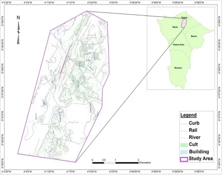
2.1. Study Area
Tarkwa Mining Community (TMC) is an area on the south-western part of Ghana and is within the Tarkwa Nsuaem Municipality. The study area is geographically located between latitudes 4° 00' 00" N and 5° 00' 00" N and longitudes 1° 45' 00" W and 2° 00' 00" W, and is about 89 km north of Takoradi, the capital of the Western Region of Ghana.
It is an old mining town which is well noted for the mining of minerals such as gold and manganese. Goldfields Ghana limited, Anglo-gold Ashanti, and Ghana Manganese Company are some of the large scale mining companies found in the TMC. There are also numerous allied mining companies located in the study area. Several small scale mining activities are also going on in the TMC. Over the past few years TMC has seen infrastructural developments including road constructions, building of health posts, education, industries, banking, hospitality services and private business development [15]. Figure 1 shows a map of the Tarkwa Mining Community.
2.2. Measurements of Field Data
The geo-spatial locations of the purpose-designed monitoring stations (PMS) in the TMC were surveyed using Garmin GPS 60CSx handheld Global Positioning System (GPS) of 2 m accuracy. A calibrated Larson Davis’s SoundTrack LxT Sound Level Meter was used to measure the noise levels in the study area. The outdoor noise levels were measured from August 2014 to January 2015. The measurements of the PMS were taken at street level and were also determined with the aid of the city digital map.
To avoid noise reflections, the noise-level meter was set on a tripod at about 1.5 m above the ground level and separated from the noise sources by at least 1.5 m. This decision was made in connection with what has been reported and accepted in the literature. For example, in [16] used 1.5 m above ground level and 1.22-1.52 m from the source of the noise. The tolerance of the calibrated Larson Davis’s Sound Track LxT trademark device is ±0.6 dBA. A-weighted instantaneous sound pressure levels were recorded three times daily at the selected positions in the study area. The total number of the points used for the modelling was 50.
2.3. Predicting Noise Pollution Levels Using MLR Approach
The noise predictive model for forecasting noise levels in the study area was developed by following the normal procedures for developing land-use regression model, using the multiple linear regression method. The noise level was defined as the dependent variable and the areas of the various land-uses within the study area were defined as independent variables.
Thus, the general equation consisted of five independent variables namely land-use, traffic intensity, road network, distance to the main road, and population density. Due to the heterogenous nature of the independent variables, they were converted into a homogeneous one that is adaptable in the multiple linear regression equation. This was done using the Analytic Hierarchy Process (AHP) of the Multi-Criteria Decision Analysis technique, which is used to solve complex multi-criteria decisions. The equations formulated from AHP were solved using matrices.
2.3.1. Application of the Analytic Hierarchy Process A mathematical expression was developed to provide weights for each criterion as a function of its rank. In computing the vector of criteria weights, a pairwise comparison matrix (A) was formulated for each pair of independent variables. The matrix A
is m x m matrix, where m is the number of evaluation criteria that was considered. Each entry ajkof matrix A represented the importance of the jth criterion compared to the kth criterion. The following conditions were set as defined in AHP procedures: if
ajk˃1, then the jth criterion is more important than the kth criterion and vice versa. If two criteria have the same importance, then the entry ajkis 1. The entries, ajkand akj satisfy the following constraint in Equation 1:
ajk.akj = 1 (1)
In this study, the importance of each factor criterion over the other was determined and quantified using the scale of pairwise comparison as developed by Saaty in the AHP [17].
The comparisons were quantified on a scale of 1 to 9. The quantity 1 represents two factors of equal importance. The quantity 9 also denotes a factor with extreme importance over the other [18]. Based on literature as well as experts’ opinion, the judgements for the independent variables were formulated. Each independent variable has five alternatives and five decision criteria. Each of the alternatives was evaluated in terms of the decision criteria and the relative importance (or weight) of each criterion.
The results are thus represented in normalized pairwise comparison matrices in proceeding Equations 2 and 3.
∑
==
m l lk jk jka
a
a
1 (2)After creating the normalized pairwise comparison matrices for the independent variables, the criteria weight vector, w is built by averaging the entries on each row of Anorm as shown in Equation 3.
m
a
w
m l jl j∑
==
1 (3)The whole processes were then summarized thus; the judgment tables was represented by 5 x 5 matrices and then squared to obtain an eigenvector. The result was then normalised by summing the eigenvector and dividing each value of the eigenvector by the sum. The weights for the individual factors were obtained after the normalisation process. The process was then repeated a number of times until the weights assigned to each factor were consistent. A consistency ratio of 0.02 was achieved which is less than the maximum allowable ratio of 0.10.
2.3.2. Applying the Multiple Linear Regression Approach The prediction model used to estimate noise pollution levels in the study area was developed using multiple linear regression approach, with matrix notation and analyses using the Statistical Package for the Social Sciences (SPSS) and MATLAB. From the multiple linear regression (MLR) model the dependent variable is related to five independent variables. The general multiple linear regression expression for k variables is as given in Equation 4.
n i e x x x
yi=
β
o+β
1 i1+β
2 i2+…+β
k ik+ i, =1,2,…, (4)In order to solve for the regression coefficient in the MLR model, as in Equation (4), the method of least squares is used. These coefficients (see Equaton 4), illustrate the unrelated contributions of each independent variable towards predicting the dependent variable. It is important to note that, the computations used in finding the regression coefficients (βi, i = 1, 2, 3, …, k), residual sum of square (SSE), regression sum of squares (SSR), etc is complex therefore, the multiple regression model in terms of observations were written using matrix notation.
This is because using matrix allows for a more compact framework in terms of vectors representing the observations, levels of regressor variables, regression coefficients, and random errors. Therefore, Equation 4 was represented in a compact as in Equation 5:
ε
β
+
=
X
Y
(5)Where, Y is noise pollution levels, X represents the independent variables; is residuals; and A is the value of Y
when all Xs are zero. After formulating the matrix equations, matrix commands in Excel were used to solve the equations and the results compared with that from SPSS software. Finally using MATLAB, the values for the coefficient of regression β, were calculated and the prediction equation was presented as in Equation 6.
ε
+
+
+
+
+
+
=
b
0b
1x
1b
2x
2b
3x
3b
4x
4b
5x
5Y
(6)Where, Y is dependent variable, what is being modelled or
predicted, x is explanatory variables, variables that influence or help explain the dependent variable, b is Coefficients, values computed by the regression equations, reflecting the relationship and strength of each explanatory variable to the dependent variable; έ is residuals, the portion of the dependent variable that isn’t explained by the model; the model under and over predictions.
The least square estimator of the coefficients of the regression equation (β) is given by Equation 7.
)
(
)
(
X
TX
−1X
TY
=
β
(7)Since X is not usually a squared matrix, it is multiplied by the transpose of X, that is XTX and the inverse of (XTX) calculated. Hence the estimator β is calculated thus using Equation 7.
The data was populated using the MATLAB software and the predicted noise levels as projected for the future were then used to develop the spatial distribution of the estimated noise levels.
2.3.3. Applying the Lyons Empirical Model
In order to confirm the developed MLR noise prediction model, the Lyons Empirical prediction model was compared to it. The Lyons Empirical Model is a mathematical model developed and applied in an area of similar conditions as that of the TMC by Lyons in [19]. The long term estimates of noise pollution levels by this model were achieved by using Equation 8.
L (Road Noise) = 10logV - 15logD + 30 logS + 10log [tanh (1.19*10-3) *VD/S] + 29 (8)
Where,
L (Road Noise) = Predicted noise level (dBA), V = Volume of traffic per hour (vehicles/hour), S = Average vehicle speed (km/hour),
D = Distance from Centre line of road.
Although the Lyons Empirical Model is a mathematical model, in this research it was considered as a “GIS only” model, since all the computations and developments were applied in the GIS environment using the Raster Calculator in ArcGIS. The mapped domain was in grid cells and the Map Algebra was used to do the calculations.
Formulating the noise map using this model, the average volume of vehicle per hour counted was 520 vehicles/hour. The average speed determined was 45 km/h and a distance map of 7 meters cell size was used. All the roads in the TMC are single carriage therefore the 7 meters cell size was used since their width is about 7 meters. The data were input into the Lyons Empirical Model and the raster calculator was used to calculate the noise map.
3. Results and Discussion
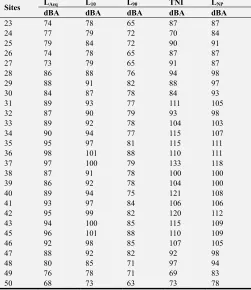
3.1. Results of the Measured Noise Levels
The results of the measured noise levels are presented in Table 1. These are presented with locations of the PMS
indicated ‘Sites’ along the major road (as explained earlier) and the computed values of noise level descriptors for the various locations in the study area.
Table 1. Average Noise Descriptors at the Monitoring Locations.
Sites LAeq L10 L90 TNI LNP
dBA dBA dBA dBA dBA
1 65 68 58 68 75
2 78 81 73 75 86
3 84 88 74 100 98
4 84 86 75 89 95
5 75 77 67 77 85
6 86 88 79 85 95
7 79 81 72 78 88
8 88 92 76 110 104
9 85 91 80 94 96
10 86 91 79 97 98
11 89 92 81 95 100
12 90 94 82 100 102
13 91 96 85 99 102
14 98 100 90 100 108
15 96 99 86 108 109
16 94 96 81 111 109
17 83 85 75 85 93
18 81 85 74 88 92
19 84 87 72 102 99
20 85 90 71 117 104
21 75 81 69 87 87
Sites LAeq L10 L90 TNI LNP
dBA dBA dBA dBA dBA
23 74 78 65 87 87
24 77 79 72 70 84
25 79 84 72 90 91
26 74 78 65 87 87
27 73 79 65 91 87
28 86 88 76 94 98
29 88 91 82 88 97
30 84 87 78 84 93
31 89 93 77 111 105
32 87 90 79 93 98
33 89 92 78 104 103
34 90 94 77 115 107
35 95 97 81 115 111
36 98 101 88 110 111
37 97 100 79 133 118
38 87 91 78 100 100
39 86 92 78 104 100
40 89 94 75 121 108
41 93 97 84 106 106
42 95 99 82 120 112
43 94 100 85 115 109
45 96 101 88 110 109
46 92 98 85 107 105
47 88 92 82 92 98
48 80 85 71 97 94
49 76 78 71 69 83
50 68 73 63 73 78
Where LAeq is A-weighted equivalent sound pressure level; L10 and L90 are the exceedence percentiles, average sound level, LD, the day-night average sound level, LDN, the noise pollution level, LNP and the traffic noise index, TNI.
3.2. Results from the Predictive Model
The results of the MLR model developed for predicting the noise levels of the study area are presented. The essence was to apply Landuse variables (POP, Traffic, Roadnet, Landuse, Distance) as input in the MLR technique to predict the level of noise within the TMC. This regression analysis allows modelling, examining, and exploring of spatial relationships. This helps to better understand the factors behind observed spatial patterns, and to predict outcomes based on that understanding.
The MLR noise prediction model developed based on the AHP principle is presented in Equation 9. The resulting correlation coefficient between the variables, summary coefficients of the multiple linear regression and others from the SPSS statistical software are presented in Table 2. The model performance based on statistical indicators is presented in Table 3.
Table 2. Coefficients of the Regression Equation.
Coefficients P-value Lower 95% Upper 95%
Intercept 68.088 5.473E-44 65.907 70.268
POP 112.602 1.38E-25 102.610 122.593
TRAFFIC -124.815 1.181E-24 -136.506 -113.123
ROADNET 36.570 4.699E-21 32.324 40.815
LANDUSE 14.146 6.624E-08 9.763 18.528
DIST 45.503 5.22E-19 39.506 51.500
Noise Levels = 112.602*(POP) – 124.815*(TRAFFIC) + 36.570*(ROADNET)
+14.146*(LANDUSE) + 45.503*(DIST) + 68.088 (9)
Table 3. Model Summary.
Mathematical Model
Performance Indicators
RMSE Mean Standard Deviation Maximum Minimum R2 R
MLR 1.569 2.462 1.585 3.718 -3.756 0.961 0.98
RME = root mean square error, R2 = coefficient of determination, R = correlation coefficient
Figure 2. Trend of Predicted and Measured Noise Levels for the Study Area.
The predicted noise levels from the MLR model is presented in Figure 2. Figure 2 shows the trend of predicted and measured values of noise level during day-night in the study.
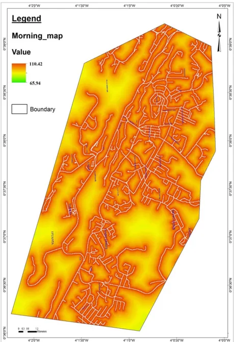
The MLR model developed was run in the MATLAB environment and the results were used to plot the spatial distribution of the noise levels of the area. The spatial distribution of the estimated noise pollution levels from the monitoring stations in the study area forecasted are presented in Figure 3 demonstrating that GIS could be used for noise mapping.
3.3. Discussion
The equivalent noise levels measured in the study area are presented in Table 1. The Table 1 shows the daily average values of noise descriptors for the monitoring stations along the major Takoradi-Tarkwa road. The monitoring stations were designated with numbers 1 to 50.
From Table 1, location 36 recorded the highest values of LAeq (98 dBA), location 37 is the next station that recorded level of LAeq (97 dBA), location 1 recorded the lowest LAeq of (65 dBA), and the station was followed by location 50. It was noted that monitoring locations with high noise descriptors were found in areas of high noise activities and vice versa. Among factors responsible for the differences in noise levels in the monitoring stations surveyed include location site, presence of intrusive noise, traffic volume, and commercial activities.
This further confirm the assertion made by [20] that noise pollution generated from ambient noise levels in a given area depend on a number of specific variables including road traffic characteristics; especially traffic volume, vehicle horn, rolling stock and tires. Some researchers have demonstrated in literature that the urban conditions of a given area are also important factor influencing the noise levels. There is a variation in the noise levels with the period of the day and the nature of the location.
Considering the regulations from Environmental Protection Agency (EPA) standards, in which equivalent sound level above 65 dBA is judged as high and could put the population at high risk, only 9 locations, representing 18%, of the 50 monitoring stations surveyed, can be classified as normally acceptable. The rest of the stations can be classified as clearly unacceptable. It is demonstrated in literature that living in areas of high noise pollution put that population in the area at risk of numerous health effects of noise pollution including, psychological, sleep and behavioural disorder as in [2] and [1]. Therefore, in comparing the values in Table 1, it could be observed that there is a danger (i.e., adverse health impact) in staying in such communities. These may results in fluctuations in the costs of house pricing in the area.
The design and implementation of noise prediction model using MLR technique yielded very good results. This will help forecast long-term variability of urban noise levels in the Tarkwa mining communities. The developed equation has brought to bear for the first time that MLR could be used to formulate noise prediction models. The results obtained, as shown in Figure 2, indicate that it is possible to develop a LUR model using the MLR technique with independent variables and that the results could be used for noise mapping as illustrated in Figure 3. The MLR produced results compared well with the study conducted by [13], which confirmed that the noise prediction model could be used in epidemiological studies.
It should be noted that Pearson correlation analysis at 0.05 significance level (two-tailed) was performed in a step wise manner on the input and output data. The essence was to
select the most suitable input parameters applicable for developing the MLR models. The results revealed that the relationship existing between POP, Traffic, Roadnet, Landuse, Distance and measured noise level are statistically significant with ρ ≤ 0.05. The interpretation is that the measured noise level provides enough convincing evidence to reject the null hypothesis and accept the alternative hypothesis that “the population correlation coefficient is different from zero” that is ρ≠0. This can be confirmed from Table 2. Therefore, in the MLR formulation, this study selected POP, Traffic, Roadnet, Landuse, and Distance as input parameters.
The performance indicators of this model, as observed in Table 3 showed RMSE, standard deviation, R2 and R values of 1.569, 1.585, 0.961 and 0.98 respectively. On the basis of quantitative evidence (Table 3), the obtained RMSE value signifies that the MLR model predictions are in consonance with the observed data. Hence, the RMSE result indicates a good statistical estimation measure of the residuals generated by the MLR model. In continuance of that, the standard deviation value shows the extent of precision of the predicted MLR results. The R2 value here indicates the tolerability of the MLR prediction values. Thus, 96.1% changes in the measured noise levels are explained by the variation in the predicted outcomes from the MLR model. The R findings, on the other hand, show the strength and direction of linear dependency existing between the observed noise levels and the predicted outputs from the MLR model. The inference made in line with the maximum and minimum values (Table 3) is that when the MLR model is applied within the study area to predict noise level a maximum error of 3.718 and minimum -3.756 could be achieved. Therefore, in this study, it is obvious that the MLR structure appears to perform satisfactorily. Figure 2 intuitively confirm this assertion where it is evident that the MLR predicted values are closely related to the observed noise levels. Therefore, it can be concluded that the statistical indicators presented in Table 3 are all within the acceptable limits.
The noise prediction model developed in this research is exclusively different from the current LUR models, since in this model a variety of independent variables are applied both in the formation of the MLR equations and application. It is also different from other basic prediction models by the consideration of land-use and other relevant variables. The results from this modelling process show that, with accurate data, noise prediction models are now promising tools, as demonstrated, for noise exposure assessment with potential applications in urban planning, epidemiological studies and environmental management, particularly in areas where noise predictions models or noise maps from competent authorities are not available.
4. Conclusion
sub-region, using MLR method. The statistical indicators used to verify the viability of the developed MLR model showed a RMSE of 1.569, standard deviation of 1.585, correlation coefficient (R) of 0.98 and R2 of 0.961. These statistical findings have revealed that the developed LUR based on the MLR could be used for noise prediction of an area with an accuracy of 98%. This assertion is based on the R of 0.98 obtained in this study. The use of R as a model assessor is in line with the study of [6] and [5] who also used the same approach for the model adequacy. Furthermore, results obtained from the MLR model is in consonance with the standard noise model (Lyons Empirical model). This was noticed from the visual observation from the noise maps produced in Figures 3 and 4.
The developed MLR model had also demonstrated its use in mapping intraurban noise in relation to urban land-use as changes occur. This is useful for urban planning and environmental noise management. It could also be applied predict intraurban noise changes with time and epidemiological studies as well as decision-making tool. It was observed from the study that the more the monitoring stations, the better the model performance. Therefore, the model performs better for large scale area like the study area and vice versa.
References
[1] Goines, L. and Hagler, L. (2007), Noise Pollution: A Modern Plaque, Southern Medical Journal, Vol. 100, Pp. 287-294. [2] Essandoh, P. K. and Armah, F. A., (2011), “Determination of
Ambient Noise Levels in the Main Commercial Area of Cape Coast, Ghana”, Research Journal of Environmental and Earth Science, Vol. 3 (6), pp. 637-644.
[3] Ozer, S., Murat, Y. and Yılmaz, H. (2009), “Evaluation of Noise Pollution Caused By Vehicles in the City of Tokat, Turkey”, Scientific Research and Essay, Vol. 4, No. 11, pp. 1205-1212.
[4] Alberola, J., Flindell, H. and Bullmore, J. (2005), “Variability in Road Traffic Noise Levels”, European Commission, Environmental Noise Directive 2002/49/EC, Off. J. European Communities L189, pp. 12-25.
[5] Lebiedowska, B. (2005), “Acoustic Background and Transport Noise in Urbanised Areas: A Note on the Relative Classification of the City Soundscape”, Trans. Res. Part D: Transport and Environment, Vol. 10, No. 4, pp. 341-345. [6] Morillas, B. J. M., Escobar, G. V., Vaquero, J. M., Sierra, M. J.
A. and Gómez, V. R. (2005), “Measurement of Noise Pollution in Badajoz City, Spain”, Acta Acustica United with Acustica, Vol. 91, No. 4, pp. 797-809.
[7] Pucher, J., Korattyswaropam, N., Mittal, N., and Ittyerah, N. (2005), “Urban transport crisis in India”, Transportation Policy, Vol. 12, No. 3, pp. 185-198.
[8] Tansatcha, M., Pamanikabud, P., Brown, A. L. and Affum, J. K. (2005), “Motorway Noise Modelling Based on Perpendicular Propagation Analysis of Traffic Noise”, Applied Acoustics, Vol. 66, No. 10, pp. 1135-1150.
[9] Zannin, P. H. T., Calixto, A., Diniz, F. B. and Ferreira, J. A. C. (2003), “A Study of Urban Noise Annoyance in a Large Brazilian City: The Importance of a Subjective Analysis in Conjunction with Objective Analysis”, Environmental Impact Assessment, Rev., Vol. 23, pp. 245-255.
[10] Benfield, J. A., Nurse, G. A., Jakubowski, R., Gibson, A. W., Taff, B. D., Newman, P., and Paul A. Bell, P. A., (2014), “Testing Noise in the Field: A Brief Measure of Individual Noise Sensitivity”, Environment and Behavior, Vol. 46 (3), pp. 353–372.
[11] Ighoroje, A. D. A, Marchie, C., and Nwobodo, E. D. (2004), Noise-Induced Hearing Impairment as an Occupational Risk Factor among Nigerian Traders, Nigerian Journal of Physiological Sciences 19 (1-2): 14-19, Physiological Society of Nigeria 2004.
[12] Passchier-Vermeer, W., and Passchier, W. F., (2000), Noise Exposure and Public Health, Environmental Health Perspective, Vol. 108, p. 123-131.
[13] Aguilera, I., Foraster, M., Basagaña, X., Corradi, E., Deltel, A., Morelli, X., Phuleria, H. C., Ragettli, M. S., Rivera, M., Thomasson, A., Rémy Slama, R., and Künzli, N., (2015), “Application of Land-use Regression Modelling to Assess the Spatial Distribution of Road Traffic Noise in Three European Cities.”, Journal of Expo Science Environ Epidemiol. Vol. 25 (1): 97-105.
[14] Xie, D., Liu, Y., and Chen, J., (2011), “Mapping Urban Environmental Noise: A Land Use Regression Method”, Environmental, Science and Technology, Vol. 45, 7358–7364. [15] Kumi-Boateng, B. (2012), “A Spatio-Temporal Based
Estimation of Land-Use Cover Change and Sequestered Carbon in the Tarkwa Mining Area of Ghana”, PhD Thesis, University of Mine and Technology, Tarkwa, 2012, pp. 163. [16] Mehdi, M. R., Minho, K., Jeong, C. S. and Mudassar, H. A.
(2010), “Spatio-Temporal Patterns of Road Traffic Noise Pollution in Karachi, Pakistan”, Environment International journal, Vol. 12, pp. 1-8.
[17] Saaty, T. L. (1980), The Analytical Hierarchy Process, McGraw-Hill, pp. 23-157.
[18] Saaty, T. (2008), “Decision making with the analytic hierarchy process”, Journal of Services Sciences, Vol. 1, No. 1, pp. 83-99.
[19] Slaboch, P. and Morris, S. (2006), “Sound and vibration produced by an airfoil tip in a turbulent boundary layer flow with an elastic endwall,” 12th AIAA/CEAS Aeroacoustics Conference, Cambridge, MA, USA, pp. 879-895.