Weighted Clustering and Evolutionary Analysis of Hybrid Attributes Data Streams

Weighted Clustering and Evolutionary Analysis

of Hybrid Attributes Data Streams

Chen Xinquan

Shangrao Normal University/Department of Mathematics and Computer, Shangrao, China Email: [email protected]

Abstract—It presents some definitions of projected cluster and projected cluster group on hybrid attributes after having given some definitions on ordered attributes and sorted attributes to solve clustering analysis problem of infinite hybrid attributes data streams in finite space. In order to improve the clustering quality of hybrid attributes data streams, it presents a two-step projected clustering method, which can often make better clustering effects in two simulated experiments although it is very simple. At last, it gives a dividing and merging framework of infinite hybrid attributes data streams. In order to implement this framework, it presents 8 properties in Section IV, some data structure definitions and 15 algorithms in appendix. The framework is verified and these algorithms are tested by German data set with a better clustering quality than WKMeans sometimes if having set right parameters.

Index Terms—ordered attributes, sorted attributes, hybrid attributes, projected clustering, merging clusters, subtracting of clusters, merging cluster groups, evolutionary analysis of cluster groups

I. INTRODUCTION

Clustering is to partition a data set into several disjoint groups so that data points in the same group are near to each other according to some distance metric. Clustering data streams has become an important research direction in data mining since 2000. It is a more challenging problem for high dimensionality, clustering speed, clustering precision, clustering meaning, data sparsity, noise or outliers, and so on. Weighted clustering and evolutionary analysis of hybrid attributes data streams should be an important research direction because of the large number of practical applications.

Joshua Zhexue Huang et al. [1] proposed WKMeans algorithm which was implemented as a component in AlphaMiner [2] after combining k-means clustering algorithm with feature-weighting. Wang X.Z. et al. [3] gave an improved FCM algorithm after a feature-weighting research in FCM clustering algorithm.

For traditional static data sets, there are already many research papers about projected clustering, subspace clustering, and so on. Aggarwal C. et al. [4] proposed a projected data stream clustering method called HPStream.

Gabriela Moise et al. [5] presented a projected clustering method, P3C, which can deal with both numerical and categorical data. Aggarwal C. et al. [6] proposed CluStream framework, which contains online micro-cluster maintenance and macro-micro-cluster creation. CluStream can only handle numerical data streams, so it is a valuable research direction to find some framework and methods which can handle both numerical and categorical data streams. In order to solve this difficult problem it gives a dividing and merging framework of infinite hybrid attributes data streams in this paper.

This paper is organized as follows. Section II gives some definitions of hybrid attributes data streams. In Section III, it presents a two-step projected clustering method of hybrid attributes data streams. Section IV presents a dividing and merging framework of hybrid attributes data streams. Section V gives several simulated experiments for the two-step projected clustering method and the dividing and merging framework. Conclusions and future work are presented in Sections VI.

II. SOME DEFINITIONS OF HYBRID ATTRIBUTES DATA

STREAMS

>

×

×

×

×

×

<

A

A

_m

A

_m+

A

_m+m

,

T

2 1 1

1 1

1

L

L

is a

domain description of m(m = m1+m2) dimensions data stream marked by a time stamp for every data point. In this m dimensions space, which contains m1 ordered attributes and m2 sorted attributes, these is a data stream

} , , , , ,

{< _{1 1} >_L < > _L

= X T XN TN

SD , where

) , , ( _{i1 im}

i x x

X = _L (i=1,_L,N,_L) is the i-th data point and Ti(i=1,L,N,L) is the i-th time stamp.

A. Some definitions of projected cluster and projected cluster group on ordered attributes

Definition 1(Projected cluster on ordered attributes)

A projected cluster DSC1

=

{

,

,

,

,

}

1

1

>

<

>

<

n

n i

i i

i

T

X

T

X

_L

of a m dimensions

data stream subset DSm

=

{

,

,

,

,

}

1

1

>

<

>

<

N

N j

j j

j

T

X

T

X

_L

on m1 ordered

attributes can be defined as a five-member group DSorder(Cluster) =

<

CF

CF

cf

cf

n

>

t t x x

,

1

,

2

,

1

,

2

(1)

This projected cluster structure DSorder(Cluster) is constructed according to the cluster structure of CluStream [6] and [8]. In formula (1),

)

2

,

,

2

(

2

1

1

x m x

x

CF

CF

CF

=

_L

, in which

( )

∑

=

= in

i j

jk x

k x

CF

1

2

2

(

k

=

1

,

L

,

m

1

)

is the square sum of

the k-th dimension values of data points in DSC1.

)

1

,

,

1

(

1

1

1

x m x

x

CF

CF

CF

=

_L

, in which

∑

=

= in

i j

jk x

k x

CF

1

1

(

k

=

1

,

L

,

m

1

)

is the sum of the k-th

dimension values of data points in DSC1.

( )

∑

=

= in

i j

j t

T cf

1 2

2 is the square sum of time stamps of data

points in DSC1.

∑

=

=

in i j

j t

T

cf

1

1

is the sum of time stamps of data points in

DSC1.

n is the number of data points in DSC1.

Definition 2(Projected cluster group on ordered attributes)

A projected cluster group of a m dimensions data stream subset DSm =

{

<

X

j₁

,

T

j₁

>

,

L

,

<

X

j_N

,

T

j_N

>

}

on m1 ordered attributes can be defined as a three-member group [8]

DSorder(Cluster group) = (W1, K1, p1) (2) In formula (2),

)

,

,

(

1

1

1

w

w

m

W

=

_L

is the weighted feature vector of

data stream subset DSm on m1 ordered attributes.

K1 is the number of projected clusters in this projected cluster group.

p1 is the pointer that points a data structure storing K1 projected clusters of this projected cluster group. B. Some definitions of projected cluster and projected cluster group on sorted attributes

Definition 3(Projected cluster on sorted attributes, the first definition)

A projected cluster DSC2

=

{

,

,

,

,

}

1

1

>

<

>

<

n

n i

i i

i

T

X

T

X

_L

of a m dimensions

data stream subset DSm

=

{

,

,

,

,

}

1

1

>

<

>

<

N

N j

j j

j

T

X

T

X

_L

on m2 sorted

attributes can be defined as a five-member group DSsort(Cluster) =

<

VF

ND

cf

cf

n

>

t t

,

1

,

2

,

,

(3)

This projected cluster structure DSorder(Cluster) is constructed extendedly according to the cluster structure of CluStream [6]. In formula (3),

)

,

,

(

2 1

1 1 m m

m

VF

VF

VF

=

₊

_L

₊ , in which

k

VF

(

k

=

m

₁

+

1

,

_L

,

m

₁

+

m

₂

)

is the most frequent value of data points in DSC2 in the k-th dimension.

Especially,

VF

k makes null when values of data points

in DSC2 in the k-th dimension are equally distributed in

its domain.

)

,

,

(

2 1

1 1 m m

m

ND

ND

ND

=

₊

_L

₊ , in which

k

ND

(

k

=

m

₁

+

1

,

_L

,

m

₁

+

m

₂

)

is the number of data points in DSC2 different from

VF

k in the k-th dimension.

( )

∑

=

= n

i

i j

j t

T cf

1 2

2 is the square sum of time stamps of data

points in DSC2.

∑

=

= in

i j

j t

T cf

1

1 is the sum of time stamps of data points in

DSC2.

n is the number of data points in DSC2.

Note:

(

,

,

)

2 1

1 1 m m

m

VF

VF

VF

=

₊

_L

₊ of Definition 3 is

similar to center vector,

and

(

,

,

)

2 1

1 1 m m

m

ND

ND

ND

=

₊

_L

₊ is similar to

standard deviation.

Definition 4(Projected cluster group on sorted attributes)

A projected cluster group of a m dimensions data

stream subset DSm =

{

,

,

,

,

}

1

1

>

<

>

<

N

N j

j j

j

T

X

T

X

_L

on m2 sorted attributes can be defined as a three-member group

DSsort(Cluster group) = (W2, K2, p2) (4) In formula (4),

)

,

,

(

2 1

1 1

2

w

m

w

m m

W

=

₊

_L

₊ is the weighted feature

vector of data stream subset DSm on m2 sorted attributes. K2 is the number of projected clusters in this projected cluster group.

p2 is the pointer that points a data structure storing K2 projected clusters of this projected cluster group. Definition 5(Projected cluster on sorted attributes, the second definition)

A projected cluster DSC2

=

{

,

,

,

,

}

1

1

>

<

>

<

n

n i

i i

i

T

X

T

X

_L

of a m dimensions

data stream subset DSm

=

{

,

,

,

,

}

1

1

>

<

>

<

N

N j

j j

j

T

X

T

X

_L

on m2 sorted

attributes can be defined as a four-member group: DSsort(Cluster) =

<

AF

cf

cf

n

>

t t

,

1

,

2

,

(5)

This projected cluster structure DSorder(Cluster) is constructed extendedly according to clustering result tree of Wkmeans in AlphaMiner [2] and cluster structure of CluStream [6]. In formula (5),

)

,

,

(

2 1

1 1 m m

m

AF

AF

AF

=

₊

_L

₊ , in which

k

AF

(

k

=

m

₁

+

1

,

_L

,

m

₁

+

m

₂

)

is dependent on the domain values of the k-th dimension. Suppose

k k

a

AF

=

is the number of the domain values of the k

-th dimension, -then

)

,

,

,

,

(

<

_{1 1}

>

<

>

=

k

k ka

ka k

k

k

v

n

v

n

AF

_L

can denote ak

points in the k-th dimension. In order to handle conveniently, ak different sort values are arranged orderly.

( )

∑

=

= in

i j

j t

T cf

1 2

2 is the square sum of time stamps of data

points in DSC2.

∑

=

= in

i j

j t

T cf

1

1 is the sum of time stamps of data points in

DSC2.

n is the number of data points in DSC2.

Note: In clustering result tree of WKMeans [2], it records various sort values and its corresponding number of data points of this cluster for ordered attributes, and it also records means and standard deviation for sorted attributes. The cluster structure in this paper can records more detail information. When sorted attributes make too many values, this cluster structure will be too large.

C. Some definitions of cluster and cluster group on hybrid attributes

Definition 6(cluster on hybrid attributes, the first definition)

A cluster DSC =

{

,

,

,

,

}

1

1

>

<

>

<

n

n i

i i

i

T

X

T

X

L

of

a m dimensions data stream subset DSm

=

{

,

,

,

,

}

1

1

>

<

>

<

N

N j

j j

j

T

X

T

X

_L

can be defined as a

seven-member group

DS(Cluster) =

<

CF

2

x

,

CF

1

x

,

VF

,

ND

,

cf

2

t

,

cf

1

t

,

n

>

(6) In formula (6),

)

2

,

,

2

(

2

1

1

x m x

x

CF

CF

CF

=

_L

, in which

( )

∑

=

= in

i j

jk x

k x

CF 1

2

2

(

k

=

1

,

L

,

m

1

)

is the square sum of

the k-th dimension values of data points in DSC.

)

1

,

,

1

(

1

1

1

x m x

x

CF

CF

CF

=

_L

, in which

∑

=

= in

i j

jk x

k x

CF 1

1

(

k

=

1

,

L

,

m

1

)

is the sum of the k-th

dimension values of data points in DSC.

)

,

,

(

2 1

1 1 m m

m

VF

VF

VF

=

₊

_L

₊ , in which

k

VF

(

k

=

m

₁

+

1

,

_L

,

m

₁

+

m

₂

)

is the most frequent value of data points in DSC in the k-th dimension. Especially,

VF

_k makes null when values of data points in DSC in the k-th dimension are equally distributed in its domain.

)

,

,

(

2 1

1 1 m m

m

ND

ND

ND

=

₊

_L

₊ , in which

k

ND

(

k

=

m

₁

+

1

,

_L

,

m

₁

+

m

₂

)

is the number of data points in DSC different from

VF

_k in the k-th dimension.

( )

∑

=

= in

i j

j t

T cf

1

2

2 is the square sum of time stamps of data

points in DSC.

∑

=

= in

i j

j t

T cf

1

1 is the sum of time stamps of data points in

DSC.

n is the number of data points in DSC.

Definition 7(cluster on hybrid attributes, the second definition)

A cluster DSC =

{

,

,

,

,

}

1

1

>

<

>

<

n

n i

i i

i

T

X

T

X

_L

of a

m dimensions data stream subset DSm

=

{

,

,

,

,

}

1

1

>

<

>

<

N

N j

j j

j

T

X

T

X

_L

can be defined as a

six-member group:

DS(Cluster) =

<

CF

2

x

,

CF

1

x

,

AF

,

cf

2

t

,

cf

1

t

,

n

>

(7) In formula (7),

)

2

,

,

2

(

2

1

1

x m x

x

CF

CF

CF

=

_L

, in which

( )

∑

=

= in

i j

jk x

k x

CF

1 2

2

(

k

=

1

,

L

,

m

1

)

is the square sum of

the k-th dimension values of data points in DSC.

)

1

,

,

1

(

1

1

1

x m x

x

CF

CF

CF

=

_L

, in which

( )

∑

=

= in

i j

jk x

k x

CF

1

1

(

k

=

1

,

L

,

m

1

)

is the sum of the k-th

dimension values of data points in DSC.

)

,

,

(

2 1

1 1 m m

m

AF

AF

AF

=

₊

_L

₊ , in which

k

AF

(

k

=

m

₁

+

1

,

_L

,

m

₁

+

m

₂

)

is dependent on the domain values of the k-th dimension. Suppose

k k

a

AF

=

is the number of the domain values of the k

-th dimension, -then

)

,

,

,

,

(

<

1 1

>

<

>

=

k

k ka

ka k

k

k

v

n

v

n

AF

_L

can denote ak

different sort values and its corresponding number of data points in the k-th dimension. In order to handle conveniently, ak different sort values are arranged orderly.

( )

∑

=

= in

i j

j t

T cf

1 2

2 is the square sum of time stamps of data

points in DSC.

∑

=

= in

i j

j t

T cf

1

1 is the sum of time stamps of data points in

DSC.

n is the number of data points in DSC.

Definition 8(cluster group on hybrid attributes)

A cluster group of a m dimensions data stream subset DSm =

{

<

X

j₁

,

T

j₁

>

,

L

,

<

X

j_N

,

T

j_N

>

}

can be defined

as a three-member group:

DS(Cluster group) = (W, K, p) (8) In formula (8),

)

,

,

,

,

,

(

2 1 1

1 1

1

w

m

w

m

w

m m

w

W

=

_L

₊

_L

₊ is the weighted

feature vector of data stream subset DSm on m hybrid

attributes.

D. Constructing method of cluster and cluster group on hybrid attributes

Because one section of hybrid attributes data stream which can be seen as a static data set and be loaded into EMS memory, its cluster group can be obtained by the following two-step projected clustering method. And its cluster data structure can be computed according to the cluster’s data points. Another constructing method of cluster group can use WKMeans [2] or weighted FCM algorithm [7].

III. TWO-STEP PROJECTED CLUSTERING METHOD OF

HYBRID ATTRIBUTES DATA STREAMS

A. Two-step projected clustering method

Suppose DSorder(Cluster group)=

{

1

,

,

1

}

1

1

C

K

C

_L

is a

projected clustering result of data stream subset DSm on

m1 ordered attributes and DSsort(Cluster group)=

}

2

,

,

2

{

2

1

C

K

C

_L

is a projected clustering result of data stream subset DSm on m2 sorted attributes.

)

,

,

1

(

1

i

K

₁

C

_i

=

_L

is a cluster of DSorder(Cluster group) which is a set containing label information of its data points, and it is the same with

C

2

_j

(

j

=

1

,

_L

,

K

₂

)

for DSsort(Cluster group).

After having merged DSorder(Cluster group) and DSsort(Cluster group), we can obtain a clustering result of data stream subset DSm on hybrid attributes.

The two-step projected clustering method:

DS(Cg) = { }; //this cluster group records clustering result on hybrid attributes. Cluster group abbreviates Cg. for (i = 1; i ≤K1; i++)

{ for (j = 1; j ≤K2; j++) {

DS(Cg) = DS(Cg)

∪

{C1i∩ C2j};

} }

B. Improvement of two-step projected clustering method The time complexity of the original two-step projected

clustering method is

}) 2 { max } 1 { max (

2

1 1, ,

, , 1 2

1 j

K j i K

i C C

K K O

L

L =

= ⋅

⋅

⋅ , because the

simple algorithm getting intersection of two sets needs

}) 2 { max } 1 { max (

2

1 1, ,

, ,

1 K i j K j

i C C

O

L

L =

= ⋅ . The time complexity

of getting intersection algorithm can be reduced if ordering the two sets DSorder(Cg)=

{

C

1

1

,

L

,

C

1

K₁

}

and

DSsort(Cg)=

{

C

2

1

,

L

,

C

2

K₂

}

at first. The best time

complexity of the ordering algorithm for DSorder(Cg) and

DSsort(Cg) is

}) 2 log 2 { max }

1 log 1 { max (

2

1 1, ,

2 ,

, 1

1 j j

K j i

i K

i C C K C C

K

O ⋅ ⋅ + ⋅ ⋅

=

= L L

.

Suppose the two ordered sets are CO1i and

CO2j(i=1,L,K1;j=1,L,K2), then its time complexity of getting intersection algorithm is O(CO1_i +CO2_j).

It is also equal to

)

2

1

(

C

i

C

j

O

+

(i=1,L,K1;j=1,L,K2). So the time complexity of the improved two-step projected clustering method is

}) 2 1 { max }

2 log 2 { max } 1 log 1 { max (

2 1 2

1

, , 1 , , 1 2 1 ,

, 1 2 ,

, 1

1 i j

K j

K i j j K j i i K

i C C K C C K K C C

K

O ⋅ ⋅ + ⋅ ⋅ + ⋅ ⋅ +

= = =

=

L L L

L

C. Getting intersection from two ordered sets

Input: Two ordered sets S1=

{

X

1

,

L

,

X

n1

}

and S2=

{

Y

1

,

L

,

Y

n2

}

.

Output: S = { }; //S records the intersection of S1 and S2. Initial S is null.

Procedure: int i = 1; j = 1;

while (i ≤ n1 && j ≤ n2) {

if (Xi == Yj) {

S = S

∪

{ Xi }; //append Xi to S

i++; j++;

} else

if (Xi < Yj) i++; else

j++; }

if (i ≤ n1)

for (k = i; k ≤ n1; k++) {

S = S

∪

{ Xk };

} //append remanent elements in S1 to S if (j ≤ n2)

for (k = j; k ≤ n2; k++) {

S = S

∪

{ Xk };

} //append remanent elements in S2 to S

Note: This is a simple method getting intersection from two ordered sets. Here it is listed independently only for integrality although it should not be the first method.

IV. DIVIDING AND MERGING FRAMEWORK OF HYBRID

ATTRIBUTES DATA STREAMS

B. Merging stratery of hybrid attributes data streams We can use a weighted clustering algorithm on hybrid attributes or two-step projected clustering method for each data stream section in order to get its cluster data structure which saves its some necessary information. How to select a merging strategy is often based on application.

1) Merging and subtracting of projected clusters and projected cluster groups on ordered attributes

The addition of projected clusters and the merging of projected cluster groups can get some summary information in some range in order to obtain cluster distributed status of data stream on ordered attributes. The subtraction of projected clusters and projected cluster groups can be used to do an evolutionary analysis of data stream on ordered attributes. This is the difference from CluStream [6]. Their implementation methods can be found in [6] and [8].

2) Merging and subtracting of projected clusters and projected cluster groups on sorted attributes

a) Merging and subtracting of projected clusters on sorted attributes

If we use the first definition(see Definition 3) for projected cluster on sorted attributes, then the merging judgement condition of DSsort(Cluster1) and DSsort(Cluster2) can be designed as

VF(Cluster1) = VF(Cluster2) (9) Property 1 (the first additive property of projected cluster on sorted attributes)

Suppose C1=

<

VF

1

,

ND

1

,

cf

2

1

,

cf

1

1

,

n

1

>

t t

and C2=

<

VF

2

,

ND

2

,

cf

2

2

,

cf

1

2

,

n

2

>

t t

are two projected clusters being able to merge on sorted attributes(satisfied VF1=VF2). Then their merged cluster can be represented as

C=C1+C2=

>

+

+

+

+

<

VF

,

ND

1

ND

2

,

cf

2

1

cf

2

2

,

cf

1

1

cf

1

2

,

n

1

n

2

t t t t

(10) In formula (10), VF = VF1 = VF2.

Property 2 (the first subtractive property of projected cluster on sorted attributes)

Suppose C1=

<

VF

1

,

ND

1

,

cf

2

1

,

cf

1

1

,

n

1

>

t t

and C2=

<

VF

2

,

ND

2

,

cf

2

2

,

cf

1

2

,

n

2

>

t t

are two projected clusters being able to make subtraction on sorted attributes(satisfied VF1=VF2). Then the difference of two projected clusters can be represented as

C = C2 -C1 =

>

−

−

−

−

<

VF

,

ND

2

ND

1

,

cf

2

2

cf

2

1

,

cf

1

2

cf

1

1

,

n

2

n

1

t t t t

(11) In formula (11), VF = VF1 = VF2.

The above two properties is obvious according to its definition.

If we use the second definition(see Definition 5) for projected cluster on sorted attributes, then the merging judgement condition of DSsort(Cluster1) and DSsort(Cluster2) can be designed as

(

)

(

⋅

)

≤δ

=

∑

+

+ =

2 1

11

2 , 1 )

2 , 1 (

m m

m k

k k k k

sort C C w dis AF AF

dis (12)

In formula (12),

δ

is a threshold larger than 0,

w

_k is the merged feature weight of Cluster1 and Cluster2 in the k

-th dimension, and

(

)

_∑

=

−

= ak

j

j k j k k

k

k AF AF n n

dis

1

1 2 2

,

1

(

k

=

m

1

+

1

,

L

,

m

1

+

m

2

)

.

Property 3 (the second additive property of projected cluster on sorted attributes)

Suppose C1=

<

AF

1

,

cf

2

1

,

cf

1

1

,

n

1

>

t t

and C2=

<

AF

2

,

cf

2

2

,

cf

1

2

,

n

2

>

t t

are two projected clusters being able to merge on sorted attributes(satisfied formula (12)). Then their merged cluster can be represented as C=C1+C2=

>

+

+

+

+

<

AF

1

AF

2

,

cf

2

₁t

cf

2

t₂

,

cf

1

₁t

cf

1

t₂

,

n

₁

n

₂ (13) In formula (13), Suppose

)

,

,

(

2

1

2 1

1 1 m m

m

AF

AF

AF

AF

AF

=

+

=

₊

_L

₊ ,

)

1

,

,

1

(

1

2 1

11 m m

m

AF

AF

AF

=

₊

_L

₊ ,

)

2

,

,

2

(

2

2 1

11 m m

m

AF

AF

AF

=

₊

_L

₊ .

Here,

1

=

(

<

₁

,

1

₁

>

,

,

<

,

1

>

)

k

k ka

ka k

k

k

v

n

v

n

AF

_L

,

)

2

,

,

,

2

,

(

2

k

=

<

v

k1

n

k1

>

<

v

ka_k

n

ka_k

>

AF

_L

.

Suppose

k k k

AF

a

AF

1

=

2

=

(

k

=

m

1

+

1

,

L

,

m

1

+

m

2

)

is

the number of different sort values in the k-th dimension. Because ak different sort values are arranged orderly, so

we can add the number of data points according to corresponding sort value for two projected clusters. Then

)

,

,

,

,

,

,

(

<

1 1

>

<

2 2

>

<

>

=

k

k ka

ka k

k k

k

k

v

n

v

n

v

n

AF

_L

)

,

,

1

(

k

=

m

₁

+

_L

m

₁

+

m

₂ can be obtained by

)

2

1

,

,

,

2

1

,

(

<

1 1

+

1

>

<

+

>

=

k k

k ka ka

ka k

k k

k

v

n

n

v

n

n

AF

_L

Property 4 (the second subtractive property of projected cluster on sorted attributes)

Suppose C1=

<

AF

1

,

cf

2

1

,

cf

1

1

,

n

1

>

t t

and C2=

<

AF

2

,

cf

2

2

,

cf

1

2

,

n

2

>

t t

are two projected clusters being able to make subtraction on sorted attributes (satisfied formula (12)). Then the difference of two projected clusters can be represented as

C = C2 -C1 =

>

−

−

−

−

<

AF

2

AF

1

,

cf

2

t₂

cf

2

₁t

,

cf

1

₂t

cf

1

₁t

,

n

₂

n

₁ (14) In formula (14), Suppose

)

,

,

(

1

2

2 1

1 1 m m

m

AF

AF

AF

AF

AF

=

−

=

₊

_L

₊ ,

)

1

,

,

1

(

1

2 1

1 1 m m

m

AF

AF

AF

=

₊

_L

₊ ,

)

2

,

,

2

(

2

2 1

1 1 m m

m

AF

AF

AF

=

₊

_L

₊ .

Here,

AF

1

k

=

(

<

v

k1

,

n

1

k1

>

,

L

,

<

v

ka_k

,

n

1

ka_k

>

)

,

)

2

,

,

,

2

,

(

2

k

=

<

v

k1

n

k1

>

<

v

ka_k

n

ka_k

>

AF

_L

.

Suppose

k k k

AF

a

the number of different sort values in the k-th dimension. Because ak different sort values are arranged orderly, so

we can make subtraction of the number of data points according to corresponding sort value for two projected clusters.

Then

=

(

<

₁

,

₁

>

,

,

<

,

>

)

k

k ka

ka k

k

k

v

n

v

n

AF

_L

)

,

,

1

(

k

=

m

₁

+

_L

m

₁

+

m

₂ can be obtained by

)

1

2

,

,

,

1

2

,

(

<

_{1 1}

−

₁

>

<

−

>

=

k k

k ka ka

ka k

k k

k

v

n

n

v

n

n

AF

_L

b) The merging and evolutionary analysis of two projected cluster groups on sorted attributes

The merging and evolutionary analysis method is similar to [8].

If we use the first definition of projected cluster on sorted attributes, the merging judgement condition is VF(Cluster1) = VF(Cluster2).

If we use the second definition of projected cluster on sorted attributes, the merging judgement condition can be designed as formula (12).

3) Merging and subtracting of clusters and cluster groups on hybrid attributes

a) Merging and subtracting of clusters on hybrid attributes

Merging and subtracting of two clusters C1 and C2 on

hybrid attributes satisfied two conditions:

(1) Projected clusters of C1 and C2 on ordered attributes satisfied the merging judgement condition(see algorithm 2 in [8]).

(2) Projected clusters of C1 and C2 on sorted attributes satisfied its corresponding merging judgement condition.

The merging judgement condition on hybrid attributes is implemented in Algorithm 2 of appendix.

Property 5 (the first additive property of cluster on hybrid attributes)

Suppose

C1=

<

1 1 1

>

1 1

,

1

,

2

,

1

,

1

,

1

,

2

CF

VF

ND

cf

cf

n

CF

x x t t and

C2=

<

2 2 2

>

2 2

,

1

,

2

,

2

,

2

,

1

,

2

CF

VF

ND

cf

cf

n

CF

x x t t are

two clusters being able to merge on hybrid attributes(both satisfied VF1=VF2 on sorted attributes and satisfied its merging judgement condition on ordered attributes(see algorithm 2 in [8])). Then their merged cluster can be represented as

C = C1+C2 =

> + + + + + +

< 1 2 1 2 1 2

2 1 2 1 , 1 1 , 2 2 , 2 1 , , 1 1 , 2

2 CF CF CF VFND ND cf cf cf cf n n CF x x x x t t t t

(15) In formula (15), VF = VF1 = VF2.

Property 6(the second additive property of cluster on hybrid attributes)

Suppose C1=

<

1 1 1

>

1 1

,

1

,

2

,

1

,

1

,

2

CF

AF

cf

cf

n

CF

x x t t

and C2=

<

2 2 2

>

2 2

,

1

,

2

,

2

,

1

,

2

CF

AF

cf

cf

n

CF

x x t t are

two clusters being able to merge on hybrid attributes(both satisfied formula (12) on sorted attributes and satisfied its merging judgement condition on ordered attributes(see algorithm 2 in [8])). Then their merged cluster can be represented as

C = C1+C2 =

> + + + + + +

< 1 2 1 2 1 2

2 1 2 1 , 1 1 , 2 2 , 2 1 , 1 1 , 2

2 CF CF CF AF AF cf cf cf cf n n

CF x x x x t t t t

(16) In formula (16),

)

,

,

(

2

1

2 1

1 1 m m

m

AF

AF

AF

AF

AF

=

+

=

₊

L

₊

=

(

1

2

,

,

1

2

)

2 1 2

1 1

1 1 m 1 m m m m

m

AF

AF

AF

AF

₊

+

₊

_L

₊

+

₊ .

Here,

)

2

1

,

,

,

2

1

,

(

<

_{1 1}

+

₁

>

<

+

>

=

k k

k ka ka

ka k

k k

k

v

n

n

v

n

n

AF

_L

)

,

,

1

(

k

=

m

₁

+

_L

m

₁

+

m

₂ .

Property 7 (the first subtractive property of cluster on hybrid attributes)

Suppose

C1=

<

1 1 1

>

1 1

,

1

,

2

,

1

,

1

,

1

,

2

CF

VF

ND

cf

cf

n

CF

x x t t and

C2=

<

2 2 2

>

2 2

,

1

,

2

,

2

,

2

,

1

,

2

CF

VF

ND

cf

cf

n

CF

x x t t are

two clusters being able to make subtraction on hybrid attributes(both satisfied VF1=VF2 on sorted attributes and satisfied its merging judgement condition on ordered attributes(see algorithm 2 in [8])). Then their difference can be represented as

C = C2 -C1 =

> − − − − − −

< 2 1 2 1 2 1

1 2 1 2 , 1 1 , 2 2 , 1 2 , , 1 1 , 2

2 CF CF CF VF ND ND cf cf cf cf n n CF x x x x t t t t

(17) In formula (17), VF = VF1 = VF2.

Property 8(the second subtractive property of cluster on hybrid attributes)

Suppose

C1=

<

1 1 1

>

1 1

,

1

,

2

,

1

,

1

,

2

CF

AF

cf

cf

n

CF

x x t t and

C2=

<

2 2 2

>

2 2

,

1

,

2

,

2

,

1

,

2

CF

AF

cf

cf

n

CF

x x t t are two

clusters being able to make subtraction on hybrid attributes(both satisfied formula (12) on sorted attributes and satisfied its merging judgement condition on ordered attributes(see algorithm 2 in [8])). Then their difference can be represented as

C = C2 -C1 =

> − − − − −

< 2 1 2 1 2 1

1 2 1 2 , 1 1 , 2 2 , , 1 1 , 2

2 CF CF CF AFcf cf cf cf n n

CF x x x x t t t t

(18) In formula (18),

)

,

,

(

1

2

2 1

1 1 m m

m

AF

AF

AF

AF

AF

=

−

=

₊

_L

₊

=

(

2

1

,

,

2

1

)

2 1 2

1 1

1 1 m 1 m m m m

m

AF

AF

AF

AF

₊

−

₊

_L

₊

−

₊ .

Here, ) 1 2 , , , 1 2 ,

(< 1 1− 1> < − >

=

k k k ka ka

ka k

k k

k v n n v n n

AF _L

)

,

,

1

(

k

=

m

₁

+

_L

m

₁

+

m

₂ .

b) The merging and evolutionary analysis of two cluster groups on hybrid attributes

The merging and evolutionary analysis method is similar to [8]. We use Algorithm 9* of appendix to make an optimum merging of two cluster groups on hybrid attributes and Algorithm 15* of appendix to make an optimum difference of two cluster groups on hybrid attributes. The two algorithms use optimum match cluster-pair strategy which is used and described in [8].

According to Property 5, 6, 7, and 8, merging framework of hybrid attributes data streams only needs a linear computing(adding or subtracting) between two clusters on hybrid attributes after having searched some optimum match cluster-pairs. So the time complexity of merging framework of hybrid attributes data streams is mainly relied on Algorithm 9* and Algorithm 15* of appendix. So its time complexity is

})) , , max{ (

} , min{

(K1 K2 K1 K2 m1 m2 am₁ 1 am₁ m₂

O ⋅ ⋅ ⋅ + ⋅ + L + (19)

In formula (19), K1 and K2 are the cluster numbers of two cluster groups which will be merged or made an evolutionary analysis, m1 is the dimensional number of ordered attributes, m2 is the dimensional number of sorted attributes, and

a

k

(

k

=

m

1

+

1

,

L

,

m

1

+

m

2

)

is the number of different sort values in the k-th dimension.

V. SIMULATED EXPERIMENTS

A. Validity experiment for two-step projected clustering method

1) Data sets

a) German data set [9]

According to decision tree algorithm J8 in AlphaMiner [2], there are 31 classification rules with 78.4% classification rate when the number of leafage node is set to 8. Then the effective classification attributes are {at1,at2,at3,at4,at5,at7,at10,at13,at17, at20}, and the unused classification attributes are {at6,at8,at9,at11,at12,at14,at15,at16,at18,at19}.

b) Credit Approval data set [10]

According to J8 [2], we can obtain a classification rule set. Its effective classification attributes are {at3,at4,at9,at10,at14,at15}, and the unused classification attributes are {at1,at2,at5,at6,at7,at8,at11,at12,at13}.

2) Experimental method

The WKMeans [2] is used as the clustering algorithm in this experiment. The number of clusters is set to 2, and weight exponent is set to 2. When using ordered attributes only, WKMeans algorithm can only get one cluster. It gets the same result that the number of clusters is set to 3, or 4. When facing this plight, we use k-means in AlphaMiner [2] as the clustering algorithm.

3) Experimental results See TABLE I and TABLE II.

It defines the clustering purity number as the number of matched data points between clustering result and its class.

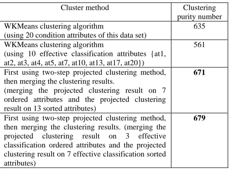
4) Analysis and conclusions of experimental results It can often get a better clustering quality than WKMeans algorithm first using two-step projected clustering method and then merging the clustering results for these two data sets. Because classification ability between ordered attributes and sorted attributes has large differences for some hybrid attributes data sets. WKMeans algorithm can not get a better clustering quality sometimes because it does not handle ordered attributes and sorted attributes rightly.

B. Validity experiment of dividing and merging framework

1) Data set

1000 data records of German data set [9] are thrown into two data sets(named German1 and German2, each has 500 records) randomly.

2) Experimental method

Do a validity experiment of merging framework like [8]. Some data structures and 15 algorithms for implementing merging framework of hybrid attributes data streams are debugged and have passed in VC++6.00. We can merge clustering results of German1 and German2 after {at1,at2,at3,at4,at5,at7,at10,at13,at17,at20} are used as input attributes in WKMeans [2]. At last do a comparison between the result using merging framework and the result using WKMeans [2].

3) Experimental results of WKMeans

Result 1: German1 has 500 records. From clustering result table of WKMeans [2], we know clust0 has 171 records and clust1 has 329 records.

361 records with tag class1 contain 112 records in clust0 and 249 records in clust1. 139 records with tag

TABLE I.

THE COMPARISON EXPERIMENTAL RESULT TABLE FOR GERMAN

Cluster method Clustering

purity number WKMeans clustering algorithm

(using 20 condition attributes of this data set)

635

WKMeans clustering algorithm

(using 10 effective classification attributes {at1, at2, at3, at4, at5, at7, at10, at13, at17, at20})

561

First using two-step projected clustering method, then merging the clustering results.

(merging the projected clustering result on 7 ordered attributes and the projected clustering result on 13 sorted attributes)

671

First using two-step projected clustering method, then merging the clustering results. (merging the projected clustering result on 3 effective classification ordered attributes and the projected clustering result on 7 effective classification sorted attributes)

679

TABLE II.

THE COMPARISON RESULT TABLE FOR CREDIT APPROVAL

Cluster method Clustering

purity number WKMeans clustering algorithm

(using 15 condition attributes of this data set)

526

WKMeans clustering algorithm

(using 6 effective classification attributes { at3,at4,at9,at10, at14,at15})

547

First using two-step projected clustering method, then merging the clustering results.

(merging the projected clustering result on 6 ordered attributes and the projected clustering result on 9 sorted attributes)

522

First using two-step projected clustering method, then merging the clustering results. (merging the projected clustering result on 3 effective classification ordered attributes and the projected clustering resulton3 effective classification sorted attributes)

class2 contain 59 records in clust0 and 80 records in clust1.

So the clustering purity number is 249+59 = 308. Result 2: German2 has 500 records. From clustering result table of WKMeans [2], we know clust0 has 258 records and clust1 has 242 records.

339 records with tag class1 contain 194 records in clust0 and 145 records in clust1. 161 records with tag class2 contain 64 records in clust0 and 97 records in clust1.

So the clustering purity number is 194+97 = 291. Result 3: German(ordered) has 1000 records. From clustering result table of WKMeans [2], we know clust0 has 560 records and clust1 has 440 records.

700 records with tag class1 contain 416 records in clust0 and 284 records in clust1. 300 records with tag class2 contain 144 records in clust0 and 156 records in clust1.

So the clustering purity number is 416+156 = 572. 4) Merged clustering result

ordered attributes: {at2,at5,at13}, sorted attributes: {at1,at3,at4,at7,at10,at17,at20}.

Using WKMeans [2] can obtain a weighted feature vector participating distance computing between two clusters for German(ordered) data set.

At last, the cluster-pair (cp1–cp4) is merged, and the cluster-pair (cp2–cp3) is also merged.

The condition of merging clusters mainly relies on the distance computing on sorted attributes. So the threshold enactment is important to the merging of clusters between two cluster groups. The merging judgement function of two clusters is Algorithm 2 in appendix.

When the threshold SortD is below 63, there is no cluster can be merged. When the threshold SortD takes 64, there are 3 clusters after german1 and german2 are merged. Because distance weight on sorted attributes is larger than on ordered attributes, the enactment of threshold is important to the merging of two clusters. Note: After having merged two cluster groups, the clustering purity number in merged clustering results is the sum of Result 1 and Result 2. So it is 308 + 291 = 599. Its clustering result with 599 is larger than Result 3 with 572.

5) Conclusions of experimental results

The merging framework is not only to solve weighted clustering problem of hybrid attributes data streams, but also can get a better clustering quality than WKMeans sometimes if having set right parameters.

VI. CONCLUSIONS

In order to solve clustering problem of hybrid attributes data streams, it presents some definitions of cluster and cluster group. In order to improve the clustering quality of hybrid attributes data streams, it presents a two-step projected clustering method, which can often make better clustering effects in two simulated experiments. In order to implement the dividing and merging framework of hybrid attributes data streams, it gives some data structures and algorithms in appendix. The framework is verified and these algorithms are tested by German data set with a better clustering quality than WKMeans [2] sometimes if having set right parameters.

It is the next work that applying the framework and its algorithms to other hybrid attributes data streams and doing a comparison with CluStream [6]. Usually, better experimental results are based on appropriate parameters. So there is more research work for adaptive optimization of parameters.

APPENDIX

The data structure definitions and 15 algorithms described by C language are listed in [11].

ACKNOWLEDGMENT

This work was supported in part by a grant No GJJ08467 from the JiangXi Provincial Department of Education, China.

REFERENCES

[1] J. Z. Huang, K. P. Ng, H. Q. Rong, et al, “Automated Variable Weighting in k-Means Type Clustering,” IEEE

Trans on pattern analysis and machine intelligence, 2005,

27(5), pp.657-668.

[2] AlphaMiner. http://bi.hitsz.edu.cn/

[3] X. Z. Wang, Y. D. Wang, and L. J. Wang, “Improving Fuzzy C-Means clustering based on feature-weight learning,” Pattern Recognition Letters, 2004, 25(10), pp.1123-1132.

[4] C. Aggarwal, J. Han, J. Wang, et al, “A Framework for Projected Clustering of High Dimensional Data Streams,” the 30th VLDB, 2004, pp.852-863.

[5] G. Moise, J. Sander, and M. Ester, “Robust projected clustering,” Knowl. Inf. Syst, 2008, 14, pp.273-298. [6] C. Aggarwal, J. Han, J. Wang, et al, “A framework for

Clustering evolving data streams,” the 29th VLDB, 2003, pp.81-92.

[7] X. Q. Chen, “Feature-weighted fuzzy C clustering algorithm,”, Computer Engineering and Design, China, 2007, 28(22), pp.5329-5333.

[8] X. Q. Chen, “Weighted clustering and evolutionary analysis facing to data streams,” http://www.paper.edu.cn, 2008, No: 200803-107.

[9] German dataset, http://www.niaad.liacc.up.pt/old/statlog/ datasets/german/german.doc.html.

[10]Credit Approval dataset, http://www.ics.uci.edu/~mlearn/ databases/credit-screening/crx.name.

[11]X. Q. Chen, “Weighted clustering and evolutionary analysis of hybrid attributes data streams” http://www.paper.edu.cn, 2008, No: 200805-29.

TABLE III.

THE COMPARISON EXPERIMENTAL RESULT TABLE FOR GERMAN

Cluster method Clustering

purity number The clustering results using WKMeans is the input

of merging framework

(merging German1 and German2)

308 + 291 =

599

WKMeans clustering algorithm for German(ordered)