Milios

(1)

Forestry & Natural-Resource Sciences Last Correction: Sep. 30, 2018

ESTIMATING TREE BOLE HEIGHT WITH BAYESIAN ANALYSIS

E. Milios

1

, K. Kitikidou

2

, E. Pipinis

3

, A. Stampoulidis

4

, M. Gotsi

5

1,2,4,5 _{Dep. of For. & Manag. of the Envir. & Nat. Res., Demokritus University of Thrace, Orestiada, Greece}

3

Fac. of Agric., For. & Nat. Envir. School of For., The Aristotle University of Thessaloniki, Thessaloniki, Greece

Abstract. The classical method for estimating a height-diameter model is based on the Least Squares

Method (LSM) and the fit of a regression line. The Bayesian method has an exclusive advantage, compared with the classical method, in that the parameters to be estimated are considered as random variables. In this study, the Simple Linear Regression (SLR) model and the Bayesian model were used to estimate bole height from breast height diameter. We used data of the forest stands of Rhodope (north-eastern Greece). variables that we used were the tree bole height and the diameter at breast height. The results showed that there is an improvement in prediction accuracy with the Bayesian model; however, this didn’t lead to narrower confidence intervals of the predicted value, compared to SLR. Narrower confidence intervals are not necessarily achieved with Bayesian methods; confidence intervals’ width is related to both statistical analyses and nature of data (in this case, species ecology and structure - composition of the stands where the sampled trees belong).

Keywords: Bayes, regression; tree height; tree bole.

1 Introduction

Forests play an important role in the wood produc-tion, recreaproduc-tion, carbon sinks and climate change (FAO

2006). Height and diameter are the most common

variables measured to estimate tree volume, site qual-ity and other important variables in forest growth and yield, species’ succession and carbon estimation models (Peng et al. 2001). Breast height diameter of individ-ual trees is easy to measure with high accuracy in the field, and minimum cost. On the contrary, tree height is not easy to estimate on standing trees; it is a time-consuming procedure, subjected to observation error, and affected by optical obstacles (Colber et al. 2002). Tree volume estimation and site quality, as well as the description of a stand’s dynamics and species’ succes-sion over time, are greatly dependent by the accuracy

of height-diameter models (Curtis 1967). There is a

series of height-diameter models, developed for several forest species (Peng et al. 2004, Temesgen et al. 2007,

Van Laar & Akca 2007). These models can be used

to estimate a missing height for a tree, while hav-ing the diameter at breast height measured (Shong-ming et al. 1992, Hann 2006), to estimate indirectly the height increment (Larsen & Hann 1987), and to estimate tree biomass applying biomass models

(Pen-ner et al. 1997). Chave et al. (2005) found that the most important parameters in biomass estimation of tropi-cal forests, in decreased order, are the breast height di-ameter, the wood density, the height and the forest’s moisture (dry forest, forest with medium or heavy mois-ture). Comprising height as a variable, in biomass mod-els, reduces significantly the standard error of biomass estimation. Therefore, an accurate tree height estima-tion should be imposed in forest inventories, simulaestima-tion models, forest management and decision support sys-tems (Peng et al. 2001, Colber et al. 2002, Curtis 1967).

Curtis (1967) compared the fit of linear

height-diameter models, in data of Douglas-fir trees (

Pseudot-suga menziesii (Mirb.) Franco). Since then, with the relatively easy fit of nonlinear models, many nonlin-ear models have been developed for estimating height

(Fekedulegn et al. 1999). However, because the tree

shape and allometry are affected by competition and environmental factors (Batziou et al. 2016, King 1991,

Kitikidou et al. 2016), any changes in these

condi-tions over time will probably affect the height-diameter relationship. This can cause uncertainty in height es-timation from the diameter. An important limitation in these models is that they produce very different re-sults, when applied in different stands from those where

(2)

they originally were developed (Calama & Montero 2004, Nogueira et al. 2008). Also, the height-diameter rela-tionship is not stable over time, even in the same stand (Flewelling & Jong 1994, Lappi 1991). These differences could have significant effects in biomass and dynamic carbon sinks. Uncertainty in height estimation, due to time changes, must be taken into account, when height-diameter relationships in natural stands are examined, and there are no available methods to resolve this prob-lem.

From all these points previously described, one can as-sess that, even a small improvement in height-diameter models, is worthy of investigation, especially regard-ing bole height, which is referrregard-ing to merchantable

vol-ume. Merchantable volume is the main interest of

forest inventories and the most contributing variable

in forest biomass and carbon sinks. Bayesian

anal-ysis is an alternative method of statistical inference, frequently used in ecological models’ evaluation (An-holt et al. 2000, Toivonen et al. 2001, Shen et al. 2003). In forestry, Bayesian methods were adopted in sev-eral applications, like the estimation of aboveground biomass (Zapata-Cuartas et al. 2012), in diameter dis-tribution (Bullock & Boone 2007) and basal area

distri-bution (Nystr¨om & St˚ahl 2001), in tree growth

estima-tion (Clark et al. 2007), mortality estimaestima-tion (Wyckoff & Clark 2000, Metcalf et al. 2009), stands’ height and volume estimation (Stewart & Weiskittel 2012), and in individual tree height estimation (Zhang et al. 2014).

Fagus sylvatica L. expands into a wide area of Europe and up to southern Scandinavia, but in the Mediter-ranean area appears only in the mountains (Korakis

2015). Fagus sylvatica is a very important tree species

for Greece, since beech forests compose 5.17% of Greek forests, while beech stands provide 20.05% of the mer-chantable volume of forests in the country (Ministry of Agriculture 1992).

In this study, we have developed Bayesian height-diameter models for beech trees, examining numerous trials from one wide study area. Since nonlinearity in a height-diameter relationship is not always detectable within an even-aged stand, due to sample sizes that can-not display lack of fit of the linear model, or excessive random variability of heights within certain diameter classes (Van Laar & Akca 2007), Simple Linear Regres-sion (SLR) models were developed. We compared the Bayesian height-diameter models to their corresponding SLR models (i.e. regression models developed with Least Squares Method (LSM)), in order to see if there is any improvement in height estimation.

2 Materials and Methods

2.1 Study area

The study was conducted in the central part of the Rhodope mountains, in the north part of the Xanthi re-gion, in north-eastern Greece (Fig. 1). The climate can be characterized as humid with harsh winters. The soils in the areas where data was collected are mainly acid brown forest soils (Dystric Cambisoils) (Milios 2000). The data were taken from areas having an elevation that ranges from approximately 580 to 1700 m.

Figure 1: Study area (wide view).

The elevation of the western part of the study area (Fig. 2, red polygon points) ranges from 1100 to 1725 m, while that of the eastern part (Fig. 2, green polygon points) ranges from 580 to 750 m.

Figure 2: Study area (large display).

In the total study area, 2809 F. sylvatica trees were

measured in plots of 500 m2 (25 m x 20 m). The plots

(3)

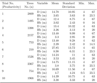
Table 1: Descriptive statistics of measured variables

Trial No. Trees Variable Mean Standard Min. Max.

(Productivity) No. (n) Deviation

1 2809 D (cm) 14.78 10.95 4 67

Hb (m) 3.65 3.63 0 23.5

2 1495 D (cm) 12.4 8.75 4 67

Hb (m) 3.02 2.43 0 16

3 1398 D (cm) 13.4 10.32 4 63

Hb (m) 3.26 3.13 0 20

4 2157 D (cm) 13.48 9.99 4 67

Hb (m) 3.3 2.95 0 20

5 753 D (cm) 13.48 9.28 4 62

Hb (m) 2.39 2.42 0 14.5

6 210 D (cm) 27.85 13.72 4 65

Hb (m) 8.98 6.31 1 23.5

7 1526 D (cm) 14.24 11 4 63

Hb (m) 3.53 3.45 0 20

8 2367 D (cm) 14.75 11.15 4 67

Hb (m) 3.8 3.75 0 23.5

9 754 D (cm) 16.69 11.56 4 67

Hb (m) 4.7 4.24 0.5 23.5

10 1968 D (cm) 14.39 10.75 4 63

Hb (m) 3.38 3.33 0 20

studies, for the analysis of stand structure and dynamics in pure and mixed stands in areas of various productiv-ities. In each tree, the breast height diameter and the bole height were measured. In particular, the measured trees came from pure beech stands in good and medium

productivity sites, from Pinus sylvestris – F. sylvatica

stands growing in good, medium and poor productivity

sites, from Fagus sylvatica – Abies borisii-regis stands

growing in medium productivity sites, and fromQuercus

petraea – Fagus sylvatica found in medium productivity

sites (Milios 2000). InP. sylvestris–F. sylvaticastands,

P. sylvestris was the dominant species of the overstorey in almost all cases (Milios 2000). From different mix-tures and productivity sites, ten different combinations (trials) were created for the analysis. Descriptive statis-tics of measured variables, in each trial, are given in Table 1.

2.2 Trial No (Productivity)

1. All

2. Good forPinus sylvestris-Fagus sylvatica, medium

forPinus sylvestris -Fagus sylvatica, and poor for Pinus sylvestris -Fagus sylvatica

3. Medium for Pinus sylvestris - Fagus sylvatica,

medium forFagus sylvatica-Abies borisii-regis, and

medium forQuercus petraea-Fagus sylvatica

(west-ern part)

forPinus sylvestris -Fagus sylvatica, poor forPinus sylvestris - Fagus sylvatica, medium for Fagus syl-vatica-Abies borisii-regis, and medium forQuercus petraea -Fagus sylvatica(western part)

5. Medium for Quercus petraea - Fagus sylvatica

(western part), and medium forQuercus petraea

-Fagus sylvatica (eastern part)

6. Good for Fagus sylvatica, and medium for Fagus

sylvatica

7. Medium for Pinus sylvestris - Fagus sylvatica,

medium for Fagus sylvatica - Abies borisii-regis,

medium forQuercus petraea-Fagus sylvatica

(west-ern part), and medium forFagys sylvatica

for Pinus sylvestris - Fagus sylvatica, medium for Fagus sylvatica - Abies borisii-regis, medium for Quercus petraea - Fagus sylvatica (western part),

good forFagus sylvatica, and medium forFagus

(4)

9. Good

10. Medium

2.3 SLR models developed with LSM

In a scatterplot with an independent ( X) variable and a dependent ( Y) variable, the goal of a linear regression model is to fit a line through the points. Specifically, with LSM, the squared deviations of the observed points from that line are minimized.

2.4 Bayesian model

Suppose y = (y1, y2, y3, ...) is a vector of data and

θ = (θ1, θ2, θ3, ...) is a vector of parameters, which will be estimated. The Bayes rule is expressed as follows:

p(y, θ) =p(y|θ)p(θ) =p(θ|y)p(y) (1)

wherepis a density probability function. While the

val-ues ofθare estimated with LSM or Maximum Likelihood

Estimation in the classical approach, in the Bayesian ap-proach we use probability distributions to describe the uncertainty in the parameters that are about to be

esti-mated. The θ have a probability distribution, which is

calculated as another form of (1):

p(θ|y) = p(y|θ)p(θ)

p(y) (2)

where p(y) = R

p(y|θ)p(θ)dθ for continuous θ. The

integration of the acceptable valuesθ,p(y) is not

depen-dent onθand can be considered as constant for constant

y, a fact that leads to the relationship (3):

p(θ|y)∝p(y|θ)p(θ) (3)

What we are interested in the Bayesian analysis is the estimation of the conditional probability, i.e., the

poste-rior probability distribution. Thep(y|θ) is giving us the

distribution ofyassuming that theθ is known, i.e., it is

the function of maximum likelihood when it is

consid-ered as a function of the θparameters (Edwards 1992).

The p(θ) is the prior probability distribution of the θ

parameters, and it represents all available information

regardingy. So, the relation (3) is suggesting that the

posterior distribution ofθis analogous to the likelihood

ofy, given theθand the prior distribution ofθ.

The important characteristic of the Bayesian analy-sis is that the models’ parameters are considered to be random variables (Stewart & Weiskittel 2012), while in the classical method of Least Squares, the models’ pa-rameters are considered fixed values (Edwards 1992, De Valpine & Hastings 2002).

The selection of the prior distribution is essential in the Bayesian analysis (Gelman et al. 2004). If there is

no available information regarding parameters’ distribu-tion, we can accept ignorance of the prior distribudistribu-tion, i.e. accept an uninformative, Gaussian prior distribu-tion.

Bayesian parameters are estimated by applying the SPSS AMOS (Analysis of Moment Structures) software, v.21.0 (Arbuckle 2012). We defined to run 100000 it-erations, from which the initial 500 were considered as initial stages of the chain before it converges (burn-in period).

2.5 Comparison of the classical and the Bayesian method

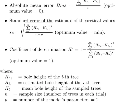
Three statistical criteria were used for the classical (SLR - LSM) and the Bayesian method comparison (Ki-tikidou 2005):

Absolute mean error Bias =

n

P

i=1

|Hb i−Hˆbi|

n

(opti-mum value = 0).

Standard error of the estimate of theoretical values

se=

s _n

P

i=1(

Hb i−Hˆbi) 2

n−p (optimum value = min).

Coefficient of determinationR2= 1−

n

P

i=1

(Hb i−Hˆbi)

2

n

P

i=1

(Hb i−Hb)

2

(optimum value = 1).

where:

Hbi = bole height of thei-th tree

ˆ

Hbi = estimated bole height of thei-th tree

Hb = mean bole height of the sampled trees

n = sample size (number of trees in each trial)

p = number of the model’s parameters = 2.

3 Results

From the ten trials of Table 1, bole height estimation was improved by applying the Bayesian method, in all of them. Comparison statistics for these ten trials, the estimated mean bole height, its confidence interval, and variance, are shown in Table 2, while SLR are shown in Table 3. We observe that in general (i.e. except for trials 2, 6, and 9), the Bayesian models gave bigger values for the estimated mean bole height, wider confidence intervals, and bigger variance.

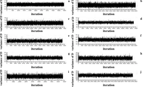
In the trace plots of Figures 3a-3j, the convergence that was succeeded by running the algorithm, is

as-sessed. The fast, up-and-down interchange, without

(5)

variance

of

D _a

variance

of

D _b

iteration iteration

variance

of

D

variance

of

D

c d

variance

of

D _e

variance

of

D f

variance

of

D _g

variance

of

D h

variance

of

D _i

variance

of

D j

Figure 3: Trace plot of the variance of the breast height diameterD (a: Trial 1, b: Trial 2, c: Trial 3, d: Trial 4, e:

Trial 5, f: Trial 6, g: Trial 7, h: Trial 8, i: Trial 9, j: Trial 10).

Table 2: Statistics for the trials in which bole height estimation was improved with the Bayesian method (SE – Standard Error; LB – Lower Bound; UB – Upper Bound; CI – Confidence Interval; EM – Estimated Mean; No – Number; ht – height).

Trial No of Classical method (SLR, LSM) Bayesian method

No trees Bias SE R2 EM CI of the EM Bias SE R2 EM CI of the EM

(n) bole ht LB UB bole ht LB UB

1 2809 2.103 3.009 0.314 3.6538 1.654 13.348 1.706 2.5702 0.499 3.8124 0.642 24.727

2 1495 1.593 2.1891 0.191 3.0204 1.999 9.6609 1.382 2.1184 0.243 2.9807 0.584 21.284

3 1398 1.756 2.5304 0.347 3.2614 1.582 12.12 1.557 2.4088 0.408 3.5916 0.73 24.595

4 2157 1.798 2.51 0.276 3.2976 1.827 11.599 1.566 2.393 0.342 3.4607 0.642 24.605

5 753 1.558 2.2673 0.126 2.3923 1.512 6.901 1.331 2.0033 0.318 2.8157 0.554 17.051

6 210 4.286 5.2663 0.306 8.9767 2.91 18.426 3.77 4.7892 0.426 5.2725 0.233 19.358

7 1526 1.898 2.7464 0.367 3.5265 1.579 12.796 1.644 2.5164 0.469 3.8676 0.731 24.728

8 2367 2.096 3.0081 0.356 3.8015 1.644 14.285 1.726 2.6168 0.513 3.9402 0.665 24.728

9 754 2.589 3.5377 0.304 4.7031 2.139 14.872 1.954 2.8066 0.562 4.1765 0.598 22.972

10 1968 1.953 2.7852 0.3 3.3775 1.619 11.607 1.633 2.4648 0.451 3.7044 0.652 24.733

In Figures 4a-4j, the autocorrelation of the values of

the variance ofD, during iterations, is illustrated. The

lag across the horizontal axis is referred to the interval in which the autocorrelation is estimated. In common situations, we expect that the autocorrelation coefficient

(6)

correlatio

n

a

variance of

D _b

Lag Lag

correlation

c

variance of

D _d

Lag Lag

correlation

e

variance of

D _f

Lag Lag

correlation

g

variance of

D _h

Lag Lag

correlation

i

variance of

D _j

Lag Lag

Figure 4: Autocorrelation of the variance of the breast height diameterD (a: Trial 1, b: Trial 2, c: Trial 3, d: Trial

4, e: Trial 5, f: Trial 6, g: Trial 7, h: Trial 8, i: Trial 9, j: Trial 10).

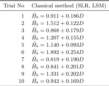
Table 3: SLR models for each trial.

Trial No Classical method (SLR, LSM)

1 Hˆb= 0.911 + 0.186D

2 Hˆb= 1.512 + 0.122D

3 Hˆb= 0.868 + 0.179D

4 Hˆb= 1.207 + 0.155D

5 Hˆb= 1.140 + 0.093D

6 Hˆb= 1.892 + 0.254D

7 Hˆb= 0.819 + 0.190D

8 Hˆb= 0.841 + 0.201D

9 Hˆb= 1.331 + 0.202D

10 Hˆb= 0.942 + 0.169D

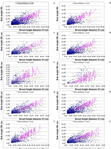
In Figures 5a-5j, the classical (SLR, LSM) vs. the Bayesian model is illustrated, for each trial, in which the Bayesian model improved the bole height estimation.

4 Discussion and Conclusions

Estimating bole height from breast height diameter, ap-plying the Bayesian method to the classical regression method (SLR, LSM) lead to an improvement of estima-tion accuracy (an increase of the coefficient of

determi-nationR2), in all our trials, conducted in the same wide

(7)

Bole height Hb (m)

0,00 5,00 10,00 15,00 20,00 25,00 30,00

0,00 10,00 20,00 30,00 40,00 50,00 60,00 70,00 80,00 Observed Bayes Linear a

Bole height Hb (m)

0,00 5,00 10,00 15,00 20,00 25,00

0,00 10,00 20,00 30,00 40,00 50,00 60,00 70,00 80,00 Observed Bayes Linear b

Breast height diameter D (cm) Breast height diameter D (cm)

Bole height Hb

(m)

0,00 5,00 10,00 15,00 20,00 25,00 30,00

0,00 10,00 20,00 30,00 40,00 50,00 60,00 70,00 Observed Bayes Linear c

Bole height Hb

(m)

0,00 5,00 10,00 15,00 20,00 25,00 30,00

0,00 10,00 20,00 30,00 40,00 50,00 60,00 70,00 80,00 Observed Bayes Linear d

Bole height Hb

(m)

0,00 2,00 4,00 6,00 8,00 10,00 12,00 14,00 16,00 18,00

0,00 10,00 20,00 30,00 40,00 50,00 60,00 70,00 Observed Bayes Linear e

Bole height Hb

(m)

0,00 5,00 10,00 15,00 20,00 25,00

0,00 10,00 20,00 30,00 40,00 50,00 60,00 70,00 Observed Bayes Linear f

Bole height Hb

(m)

0,00 5,00 10,00 15,00 20,00 25,00 30,00

0,00 10,00 20,00 30,00 40,00 50,00 60,00 70,00 Observed Bayes Linear g

Bole height Hb

(m)

0,00 5,00 10,00 15,00 20,00 25,00 30,00

0,00 10,00 20,00 30,00 40,00 50,00 60,00 70,00 80,00 Observed Bayes Linear h

Bole height Hb

(m)

0,00 5,00 10,00 15,00 20,00 25,00

0,00 10,00 20,00 30,00 40,00 50,00 60,00 70,00 80,00 Observed Bayes Linear i

Bole height Hb

(m)

0,00 5,00 10,00 15,00 20,00 25,00 30,00

0,00 10,00 20,00 30,00 40,00 50,00 60,00 70,00 Observed Bayes Linear j

(8)

to shade tolerant species, after their youth, they cannot form shade leaves (see Dafis 1986, Oliver & Larson 1996, Lacointe et al. 2004). Thus, when shade-tolerant trees with large diameters of the overstorey, grow with shade intolerant species, they grow longer crowns compared to those growing in pure stands, or mixed stands having other shade tolerant species since more light reaches the lower part of boles. In the present study, this is obvious

in all the trials where beech grows withP. sylvestris or

Q. petraea. Pinus sylvestrisis shade intolerant, whileQ. petraea is moderately shade-intolerant (Korakis 2015). In these trials, the Bayesian method overestimates the bole height of trees having large diameters, compared to the classical regression method, leading to larger confi-dence intervals (Figs. 5a-5e, Figs. 5g-5j). Only in trial 6, which is the only trial with pure beech stands (and crowns of the trees with large diameters are short) the Bayesian method does not overestimate the bole height (Fig. 5f). So, the Bayesian method does not give a pri-ori narrower confidence intervals; confidence intervals’ width is related to the characteristics of the data.

Another finding of the present study is that in both methods (classical and Bayesian), in trials from mixed

stands of P. sylvestris - F. sylvatica and/or Q. petraea

- F. sylvatica (trials 2 and 5) the R2 _{values are lower} than in the other trials. One should note that, in trials

with pure beech stands (1, 6, 7, 8, 9 and 10) the R2

values in the Bayesian method are rather high, while in some of these trials (1, 8, 9 and 10) the increase of the

R2_{, compared to the classical method, is very high. The}

lowest R2 _{value of these trials is found in trial 6, where}

trees only from pure stands participate. This pattern indicates that bole height prediction is more accurate where trees from all growth environments are present. However, even in the case where only trees from pure beech stands are present, the Bayesian method provides

a rather high R2 _{value. The behaviour of these models}

is affected by the growth characteristics and ecology of beech, which have been described previously. Probably the existence of trees from pure beech stands provides an adequate number of large trees having high bole height in the sample (small crown length is a result of competi-tion among shade-tolerant trees), improving the model’s performance.

In trial 9 (good productivity sites) the R2_{value of 0.56}

is an indication that growth conditions in different site productivities may influence the model’s performance.

However, in trial 10 (medium productivity sites) the R2

value was lower than that of trial 1.

To sum up, the Bayesian method is an important tool, used more and more by ecologists (Hui et al. 2006, Hui et al. 2011, McCarthy et al. 2007). For this specific application in bole height estimation, more independent variables could be added in the future, such as site

qual-ity index, age, or stand densqual-ity (Temesgen & Gadow 2004, Newton & Amponsah 2007).

Acknowledgements

Thanks are due to the anonymous reviewers and the MCFNS editors for their helpful comments improving the manuscript.

References

Anholt, B., Werner, E., & Skelly, D. 2000. Effect of food and predators on the activity of four larval ranid frogs, Ecology, 81 (12): 3509–3521.

Arbuckle, J. 2012. IBM SPSS Amos 21 User’s Guide, IBM Corporation, 653 p., USA.

Assmann, E. 1970. The Principles of Forest Yield Study, Pergamon Press, 506 p., New York, USA.

Batziou, M., Milios, E., & Kitikidou, K. 2016. Is di-ameter at the base of root collar a key characteristic

of seedling sprouts in a Quercus pubescens -

Quer-cus frainettograzed forest in Northeastern Greece? A morphological analysis, New Forests, 48(1): 1–16.

Bullock, B., & Boone, E. 2007. Deriving tree diameter distributions using Bayesian model averaging, Forest Ecology and Management, 242, (2–3): 127–132.

Calama, R., & Montero, G. 2004. Interregional nonlin-ear height-diameter model with random coefficients for stone pine in Spain, Canadian Journal of Forest Research, 34(1): 150–163.

Chave, J., Andalo, C., Brown, S., Cairns. M., Chambers,

J., Eamus, D., F¨olster, H., Fromard, F., Higuchi, N.,

Kira, T., Lescure, J., Nelson, B., Ogawa, H., Puig, H., Rira, B., & Yamakura T. 2005. Tree allometry and improved estimation of carbon stocks and balance in tropical forests, Oecologia, 145(1): 87–99.

Clark, J. S., Wolosin, M., Dietze, M., Ib´a˜nez, I., LaDeau,

S., Welsh, M., & Kloeppel, B. 2007. Tree growth infer-ence and prediction from diameter censuses and ring widths. Ecological Applications 17:19421953.

Colbert, K., Larsen, D., & Lootens, J. 2002. Height-diameter equations for thirteen midwestern bottom-land hardwood species., Northern Journal of Applied Forestry, 19(4): 171–176.

Curtis, R. 1967. Height-diameter and height-diameter-age equations for second-growth Douglas-fir, Forest Science, 13: 365–375.

(9)

De Valpine, P., & Hastings, A. 2002. Fitting population models incorporating process noise and observation error, Ecological Monographs, 72(1): 57–76.

Edwards, A. 1992. Likelihood. Johns Hopkins University Press, 296 p, Baltimore, USA.

FAO. 2006. GreenFacts - Scientific facts on forests. Level 2 - Details on forests, GreenFacts Foundation, 62 p, Brussels, Belgium.

Fekedulgn, D., Mac Siurtain, M., & Colbert, J. 1999. Parameter estimation of nonlinear growth models in forestry, Silva Fennica, 33(4): 327–336.

Flewelling, J., & De Jong, R. 1994. Considerations in si-multaneous curve fitting for repeated height-diameter measurements, Canadian Journal of Forest Research, 24(7): 1408–1414.

Gelman, A., Carlin, J., Stern, H., & Rubin, D. 2004. Bayesian Data Analysis, 2nd edition. Chapman and Hall/CRC, 690 p, Boca Raton, USA.

Hann, D. 2006. ORGANON User’s Manual Edition 8.0. Department of Forest Resources, Oregon State Uni-versity, 129 p, Corvallis, Oregon, USA.

Huang, S. 1999. Ecoregion-based individual tree height-diameter models for lodgepole pine in Alberta, West-ern Journal of Applied Forestry, 14(4): 186–193.

Huang, S., Titus, S., & Wiens, D. 1992:. Comparison of nonlinear height-diameter functions for major Alberta tree species, Canadian Journal of Forest Research, 22(9): 1297–1304.

Hui, C., Foxcroft, L., Richardson, D., & Macfadyen, S. 2011. Defining optimal sampling effort for large-scale monitoring of invasive alien plants: a Bayesian method for estimating abundance and distribution, Journal of Applied Ecology, 48(3): 768–776.

Hui, C., McGeoch, M., & Warren, M. 2006. A spatially explicit approach to estimating species occupancy and spatial correlation, Journal of Animal Ecology, 75(1): 140–147.

King, D. 1991. Tree allometry, leaf size and adult tree size in old-growth forests, Tree Physiology, 9(3): 369– 381.

Kitikidou, K. 2005. Applied Statistics Using SPSS, Tzi-olas Press, 288 p, Thessaloniki, Greece.

Kitikidou, K., Milios, E., & Katsogridakis, S. 2016.

Meta-analysis for the volume of Pinus sylvestris in

Europe, Revista Chapingo Serie Ciencias Forestales y del Ambiente, 23(1): 22–34.

Korakis, G. 2015. Forest Botany, Hellenic Academic Li-braries, 619 p, Athens, Greece.

Lacointe, A., Deleens, E., Ameglio, T., Saint-Joanis, B., Lelarge, C., Vandame, M., Song, G., & Daudet,

F. 2004. Testing the branch autonomy theory: a

13C/14C double-labelling experiment on differentially shaded branches, Plant, Cell and Environment, 27: 1159–1168.

Lappi, J. 1991. Calibration of height and volume equa-tions with random parameters, Forest Science, 37: 781–801.

Larsen, D., & Hann, D. 1987. Height-Diameter Equa-tions for Seventeen Tree Species in Southwest Ore-gon. Oregon State University, 16 p, Corvallis, Oregon, USA.

Li, R., Stewart, B., & Weiskittel, A. 2012. A Bayes-ian approach for modelling non-linear longitudi-nal/hierarchical data with random effects in forestry, Forestry, 85(1): 17–25.

McCarthy, M. 2007. Bayesian Methods for Ecology, Cambridge University Press, 295 p, Cambridge, UK.

Metcalf, C., McMahon, S., & Clark, J. 2009. Overcoming data sparseness and parametric constraints in model-ing of tree mortality: a new nonparametric Bayesian model, Canadian Journal of Forest Research, 39(9): 1677–1687.

Milios, E. 2000. Dynamics and evaluation of the Rho-dope mixed stands in the region of Xanthi (In Greek), PhD thesis, Aristotle University of Thessaloniki, 345 p.

Milios, E. 2004. The influence of stand development pro-cess on the height and volume growth of dominant Fa-gus sylvatica L. sl trees in the central Rhodope Moun-tains of north-eastern Greece, Forestry, 77(1): 17–26.

Ministry of Agriculture. 1992. Results of the rst national forest inventory (in Greek), Publication of Depart-ment of Forest Mapping, 134 p, Athens, Greece.

Newton, P., & Amponsah, I. 2007. Comparative evalua-tion of five height-diameter models developed for black spruce and jack pine stand-types in terms of goodness-of-fit, lack-of-fit and predictive ability, Forest Ecology and Management, 247(1–3): 149–166.

Nogueira, E., Nelson, B., Fearnside, P., Frana, M., &

Oliveira, ´A. 2008. Tree height in Brazil’s “arc of

(10)

Nystr¨om, K., & St˚ahl, G. 2001. Forecasting probability distributions of forest yield allowing for a Bayesian ap-proach to management planning, Silva Fennica, 35(2): 185–201.

Oliver, C., & Larson, B. 1996. Forest stand dynamics, 520 p, John Wiley & Sons, Inc., New York, USA.

Peng, C., Zhang, L., & Liu, J. 2001. Developing and validating nonlinear height-diameter models for ma-jor tree species of Ontario’s boreal forests, Northern Journal of Applied Forestry, 18(3): 87–94.

Peng, C., Zhang, L., Zhou, X., Dang, Q., & Huang, S. 2004. Developing and evaluating tree height-diameter models at three geographic scales for black spruce in Ontario, Northern Journal of Applied Forestry, 21(2): 83–92.

Penner, M., Power, C., Muhairve, C., Tellier, R., & Wang, Y. 1997. Canada’s forest biomass resources: deriving estimates from Canada’s forest inventory. In-formation Report BC-X-370, Canadian Forest Service, 33 p, Pacific Forestry Centre, Victoria, Canada.

Shen, T., Chao, A., & Lin, F. 2003. Predicting the number of new species in further taxonomic sampling, Ecology, 84(3): 798–804.

Temesgen, H., & Gadow, K. 2004. Generalized height-dimater models—an application for major tree species in complex stands of interior British Columbia, Euro-pean Journal of Forest Research, 123(1): 45–51.

Temesgen, H., Hann, D., & Monleon, V. 2007. Regional height-diameter equations for major tree species of southwest Oregon, Western Journal of Applied Forestry, 22(3): 213–219, 2007.

Toivonen, H., Mannila, H., Korhola, A., & Olander, H. 2001. Applying Bayesian statistics to organism-based environmental reconstruction, Ecological Appli-cations, 11(2): 618–630.

Van Laar, A., & Akca, A. 2007. Forest Mensuration. Springer, Dordrecht, 384 p, The Netherlands.

Wyckoff, P., & Clark, J. 2000. Predicting tree mortal-ity from diameter growth: a comparison of maximum likelihood and Bayesian approaches, Canadian Jour-nal of Forest Research, 30(1): 156–167.

Zapata, M., Sierra, C., & Alleman, L. 2012. Probability distribution of allometric coefficients and Bayesian es-timation of aboveground tree biomass, Forest Ecology and Management, 277: 173–179.