Thesis

By: Isabella Sun

Honors Thesis Economics Department

University of North Carolina at Chapel Hill

April 2015

Approved:

Acknowledgement

Abstract

I. Introduction

The impact of international trade on domestic unemployment is one of the major concerns of more open trade policies. While trade economists generally agree that a more open economy is good for growth and development of the economy overall, there are still other potential effects of trade, one of the most common discussions being the impact on employment. Intuitively, trade can impact unemployment in different ways through imports and exports. An increase in exports would imply an increase in domestic production. Increased domestic production would create more opportunities for domestic jobs, and thus should decrease the unemployment rate. Increased imports on the other hand would imply relatively more production abroad, and thus would have the opposite effect on jobs, increasing the unemployment rate.

ratification were arguments that NAFTA will create jobs1 _{(Davidson, Martin, & Matusz, 1999).} These numbers suggest that the major concern over trade openness is the effect it will have on jobs. This research will address these concerns by testing the null hypothesis that increased trade has no impact on the unemployment rate.

The specific focus of this research is on the impact of trade with China on the unemployment rate in Taiwan. The topic of trade between Taiwan and China is particularly relevant due to the protests that occurred recently in Taiwan over a free trade agreement with China. Taiwan has a complicated relationship with Mainland China. Many Taiwanese fear the People’s Republic of China’s growing political influence, but Taiwan also has extremely close economic ties to the Mainland. In 2013, the ruling party of Taiwan, passed the Cross-Strait Service Trade Agreement, a bilateral trade agreement with China. This event sparked the Sunflower Movement that dominated the headlines in March of that following year in protest of the FTA2_{. Such a trade agreement not only makes the entire country more susceptible to China’s} influence, but it also makes Taiwanese firms more vulnerable to foreign competition. For this reason, many Taiwanese citizens opposed the agreement due to fear that more open trade will result in the Chinese “stealing” their jobs. The protests that occurred begs the question, what impact, if any, does trade with China have on the unemployment rate in Taiwan. If more trade

does not actually impact unemployment, then the concerns of the protestors in terms of impacts on unemployment are unwarranted. If increased trade does have an impact on the unemployment rate, then the direction of this impact would have important trade policy implications. Another possibility to take into consideration is that the level of trade overall may be more important than the amount of trade specifically with China.

This research will contribute to the existing literature by looking specifically at the relationship between trade and unemployment in the case of Taiwan. Moreover, it looks at the impact of trade specifically with Mainland China where much of the previous literature is more concerned with more open trade with the rest of the world as a whole, which this research will likewise additionally examine. This research finds that there is no connection between Taiwan’s unemployment rate and trade between Taiwan and China in the long run. However, there is a statistically significant impact on the unemployment rate in the short run. Interestingly, the direction of the impact on unemployment is a positive one, indicating that increased trade with China increases the unemployment rate in Taiwan. Trade with the rest of the world as a whole, not including China, has the opposite effect where increased trade to all other countries combined decreases the unemployment rate. This research also examines the separate effects of imports and exports on the unemployment rate in Taiwan and finds statistically significant evidence that increased imports and exports both increase the unemployment rate.

has examined other aspects of the labor market such as wage rates. Other indicators of trade have also been considered in previous literature. Where this research uses data on imports and exports of goods, other literature has examined the impacts of tariffs or other trade policies for example. In section III, I present a theoretical model developed by Dutt, Mitra and Ranjan (2009, 2012), which explains the connection between trade and employment. Section IV of this paper discusses the data used for the empirical tests, which are presented in section V. The results from the empirical tests are subsequently presented in section VI with the figures and tables in the Appendix.

II. Literature Review

The economic literature on the impact of trade on employment is divided. There have been previous studies that have found no statistically significant impact of trade on employment, but there is also a considerable amount of studies that have found a statistically significant impact of trade on employment. Many empirical studies have found ambiguity in the direction of this impact or that there is a dynamic impact of trade on employment, as their results show opposite effects on employment in the short run and the long run. Overall though, the literature tends to have stronger evidence to support that increased trade reduces the unemployment rate.

the trade reforms reduced the relative wages of workers in the industries that lost protection, showing that trade does have an impact on the labor market. However, the impact found on employment was not statistically significant. Attanasio, Goldberg, and Pavcnik (2004) in examining the case of Colombia also find impacts of tariff reductions on wages, but no significant impact on unemployment. Lang (1998) similarly measured the impact of trade liberalization but in the case of New Zealand and also found no statistically significant impact of tariff reductions on employment.

Though there is literature that suggests no impact of trade on unemployment, there is also empirical evidence to suggest that increased trade does have some impact on employment. Felbermayr, Prat, and Schmerer (2011) for example ultimately conclude that a 10 percentage point increase in total trade openness reduces unemployment by three quarters of one percentage point. In much of the empirical studies that find a statistically significant relationship between trade and employment though, the evidence is ambiguous as to the direction of this impact, which will be reviewed below.

higher rate of matching. Grossman (1987) also using evidence from the United States find that the responsiveness of employment to competition from imports differed across sectors. Moreover the impacts in different sectors varied in magnitude.

Dutt, Mitra, and Ranjan (2009), and Hasan, Mitra, Ranjan and Ahsan (2012) find ambiguity in the impact of trade on unemployment in that this impact changes over time. Dutt, Mitra, and Ranjan (2009) using cross-national panel data examine the effect of various measures of trade openness across countries on unemployment rates, and their results generally show that trade openness reduces unemployment. In examining the short run and long run effects of trade liberalization, they find that permanent trade liberalization shocks increase unemployment in the short run, but these effects reverse over time and actually reduce unemployment in the long run. Empirical evidence from India presented in Hasan, Mitra, Ranjan and Ahsan (2012), also shows a possibility of increased unemployment as a result of trade liberalization, but this effect only occurs in the short run. They had more robust evidence to suggest that trade liberalization reduces unemployment especially in states with flexible labor markets.

III. Review of Theoretical Models

this model, each country will produce exclusively the product in which they have a comparative advantage. Thus all of the labor resource that had previously been allocated to the sector, in which the country did not have a comparative advantage in is then perfectly reallocated to the other sector. There is no unemployment. While this model is elegantly simple in this way, that there is zero labor market friction is a criticism of this model. One would not expect the economy to actually operate so flawlessly. Assuming in fact that all job losses are eventually perfectly offset by new job creation, this does not happen instantly. Moreover, the economy does not actually operate with perfect information so it takes time for firms to decide to fire workers and also for laid off workers to find a new job.

different effects for unemployment in different countries depending on the conditions. Trade between a small country and a large country that is more abundant in capital and has more efficient employment search technology, increases aggregate unemployment in the large country.

Helpman and Itskhoki (2010) also present a similar but more complicated theoretical model of labor and trade where trade is affected by frictions in the labor market, and impacts on unemployment are subject to the situation. In this model the two countries produces homogenous goods in one sector and differentiated goods in the other sector. The implications of this model are that trade can raise the level of unemployment if the relative labor market frictions are low in the differentiated goods sector, but trade can also lower the level of unemployment if the relative labor market frictions are high in the differentiated goods sector.

This theoretical model presented below, developed by Dutt, Mitra, and Ranjan (2009, 2012), illustrates a relationship between trade and unemployment. In this model of trade, labor (L) is the only factor of production. The economy modeled here produces a single final non-tradable good (Z), and two intermediary non-tradable goods (X and Y) with prices px and py. The production function for good Z is

Z= A X

1−α_Yα

αα

(1−α)1−α ; 0<α<1 (1)

The cost of this final good is determined by the prices of the intermediary goods and given by the equation and set equal to 1 as it is the only tradable good in the economy.

c

₍

₎

1−α pyα

Due to the nature of the production function for this final good, the relative demand for the two intermediate goods can be expressed as

Xd

Yd=

(1−α)py

α p_x

(3)

The production of the intermediary goods requires a match between workers and jobs and each pair producing only one unit of output. The rate at which these matches are made is dependent on the amount of job vacancies and the amount of unemployed individuals. Breakups are caused by exogenous shocks. The number of workers employed in each sector can be expressed as

(

X=h_x

₍

₎

₍

₎

Market tightness is expressed by a value θ_i=v_i/u_i where v_i is the vacancy rate in sector i. The flow of matches in the labor market is given by the following equation where m_{i is a scale}

parameter, and γ is a parameter that expresses the intensity of job vacancies.

M_i(v_iL_i, u_iL_i

₎

₍

₎

₍

This describes the flow into employment; so next, there must be an equation to describe the flow into unemployment. Let λ_{i be the exogenously given rate at which breakups of matches}

occurs in sector i per period.

˙

u_i= λi

λ_i+m_iθ_iγ (7)

Equation (7) gives the constant steady state rate of unemployment.

This model also includes cost of firing of employees for the employers (Fi) and a recruitment cost (δ_{i). Let} ρ be the discount factor, Vi be the asset value of a vacant job, and Ji be the value of an occupied job.

ρ Vi=−δi+miθi

γ−1

(Ji−Vi) (8)

If there is free entry in job creation, then V_i=0, and wages in sector i are denoted, wi an equation for Ji can be written

ρ Ji=pihi−wi−λi(Ji+Fi) (9)

Equation (10), the value of occupied jobs, can be derived from equation (8) when free entry in job creation is assumed.

J_i= δi

m_iθ_iγ−1 (10)

Solving equations (9) and (10) together results in

p_ih_i−w_i−λ_iF_i=δi(ρ+λi)

m_iθ_iγ−1 (11)

The left hand side of the equation shows the hiring and firing costs as well as the wage, and the right hand side of the equation shows the value of the match.

present discounted value of employment, and Ui is the present discounted value of unemployment.

ρ Wi=wi+λi(Ui−Wi) (12)

ρ Ui=b+miθiγ(Wi−Ui) (13)

Wage in this model is determined through Nash bargaining. The bargaining power of workers is given by β.

W_i−U_i= β

1−βJ (14)

Solving equations (9), (10), (12) (13), and (14) together gives the equation

w_i=(1−β)b+β(p_ih_i+δ_iθ_i−λ_iF_i) (15)

Finally, using equations (7), (11), and (15) together to obtain an equation that presents the impact of trade on unemployment.

∂θi

∂ p_i=

(1−β)h_i

δ_i(β+

(

)

m_i )

>0

(16)

∂ui

∂ p_i=

−λimiγ θiγ−1

(λ_i+m_iθ_iγ)2

∂θi

∂ p_i=−γ ui

(

)

∂ θi

∂ p_i<0 (17)

firms’ production decision. So, the relative price of the good will impact the level of exports and imports in different trading sectors. Sectors with comparative advantage will see an increase in exports whereas sectors that do not have the comparative advantage will have an increase in imports. This in turn will lead to firms increasing the number of job vacancies in sectors increasing exports, which results in a lower unemployment rate in that sector as there is a higher number of vacancies relative to the number of workers searching. Conversely, sectors where the relative price of the good decreases and thus the marginal product of labor in those sectors also decrease become import sectors. Firms in that sector will decrease job vacancies, which will increase the unemployment rate in that sector as there will be a higher number of workers searching relative to the number of vacancies.

The effect on aggregate unemployment for the whole economy depends on which sector had higher unemployment to begin with. The hypothesis of this theoretical model for the impact of trade on unemployment is thus flexible since it depends on the initial starting point of unemployment in each sector. Allowing for different results on unemployment could be useful for explaining different impacts on open trade on unemployment in different countries. It is also useful for explaining the conflicting results found in the previous literature for the effect of trade on employment.

IV. Data

aggregated for the economy in Taiwan as a whole. The aggregate unemployment rate in Taiwan data comes from the Directorate General of Budget, Accounting and Statistics. The unemployment rate is collected as a part of The Manpower Survey, which is a sampling survey of households on labor statistics in Taiwan. They survey is taken monthly of a sample of 20,000 households in Taiwan. The DGBAS provides the data on the labor force including the unemployment rate free on their website for observations monthly from January 1978 to December 2014.

Other exogenous variables used in the empirical model are the GDP per capita, average wage and a manufacturing production index. GDP per capita is provided by the DGBAS of Taiwan in US dollars at current prices quarterly from the first quarter of 1961 to the fourth quarter of 2014. Average monthly earnings in Taiwan data are provided by the DGBAS from January 1980 to December 2014 and reported in New Taiwan dollars. The manufacturing production index comes from the Ministry of Economic Affairs and Statistics Department using 2011 as the base year. The data is provided from January 1971 to December 2012.

Since time series regressions requires consecutive, evenly spaced observations, this research will analyze the time period from August 1992 to November 2014, as this is the only complete data for all necessary variables. This gives a total of 268 observations.

billion dollars in the early 90s to an average of 19.23 billion dollars in the early 2010s. Exports to the rest of the world not including China increased from an average of 7.90 billion dollars in the early 90s to an average of 18.75 in the early 2010s.

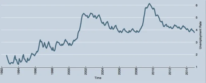
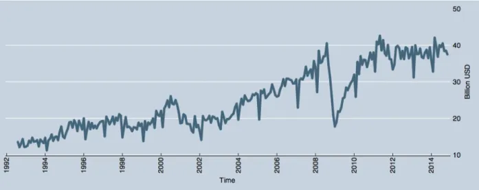
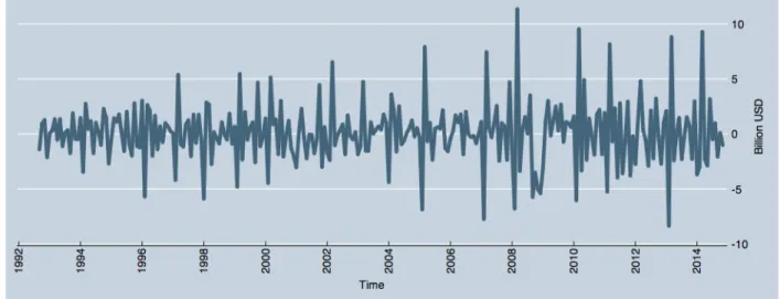
Unlike the average value of imports and exports in every sub-period, the average unemployment rate did not increase in each subsequent sub-period. In the timeframe overall there was an increase in the unemployment rate from 1.59 in the early 90s to 4.19 in the early 2010s. The sub-period with the highest average unemployment rate was the early 2000s with 4.66 percent, and this average decreased only slightly to 4.60 percent in the next sub-period, the late 2000s. Figure 1 shows the average monthly unemployment rate over time. The sudden increase in the unemployment rate around 2001 is likely due to the September 11 attack in the United States in 2001. The decrease in tourism that occurred after September 11 had a negative impact on many economies including Taiwan. The Great Recession observed around the world in 2008 can explain the next sharp increase in the unemployment rate in Taiwan around 2008. The Great Recession is also the likely cause of the sharp decreases in the level of trade with China in 2008 shown in Figure 2 as well as the sharp decrease in the level of trade with the rest of the world not including China in 2008 shown in Figure 3.

V. Empirical Model

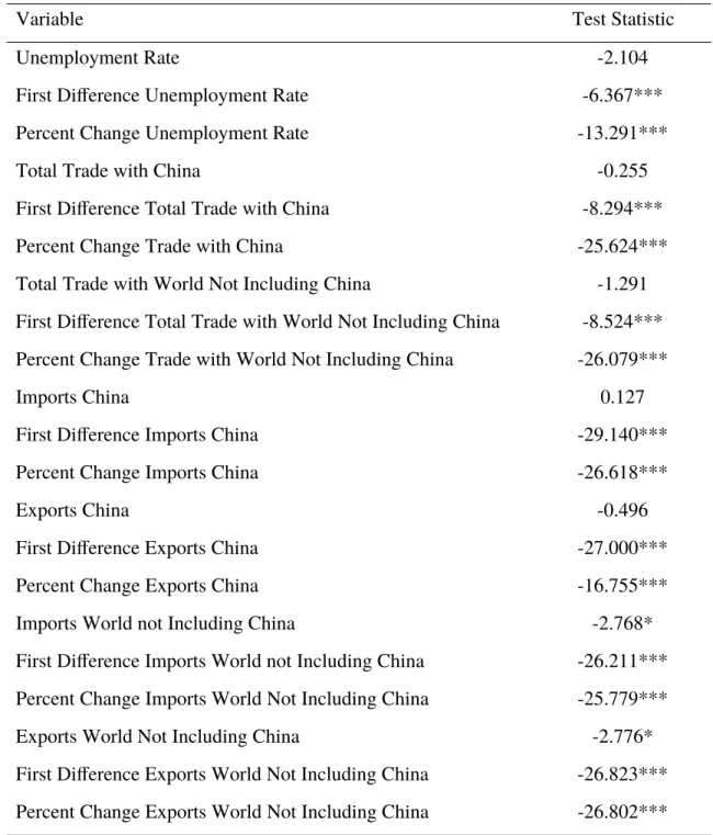
The increasing means of the variables as shown in the summary statistics over time as well as a visual analysis of the graphs of the variables, figures 1, 2, and 3, suggests the presence of a deterministic trend, meaning that the expected value of the variable is not independent of the time variable. If the expected value of a variable X_{t is not independent of the time variable} t, then Xt is nonstationary. The Dickey-Fuller test essentially allows us to test the whether

Moreover, since the relevant variables in this research, the unemployment rate, trade with China, both seem to have a general upward trend, it begs the question of whether there may be any long run relationship between the unemployment rate and trade. Generally speaking, a linear combination of time series variables will be stationary if at least one of them is non-stationary. However, if there is a long run relationship between two time series variables, then it could be that a linear combination of those time series variables is stationary, so they share a common stochastic drift. When time series variables share a common stochastic drift, then they are cointegrated. The Johansen Cointegration test allows us to test for cointegration.

To test short run causality I use a vector autoregressive model and Granger Causality test. The main empirical model is as follows

UR_t=α+

∑

l=1 4

β_t−lUR_t−l+

∑

l=1 4

γ_t−lX_t−l+

∑

l=1 4

δ_t−lY_t−l+

∑

i

μ_iA_i+ε_t

The εtis the disturbance term. There are several assumptions on εt in a time series

regression. First, it is assumed that the disturbance term has an expected value of 0. Secondly, the disturbance term is homoscedastic. Thirdly, the disturbance terms have independent distributions. Fourthly, the disturbance term is distributed independently of the other variables on the right hand side of the equation. Fifthly, the disturbance term is normally distributed.

∑

μ_iA_{i represents the exogenous controls included in the model. This includes the GDP}

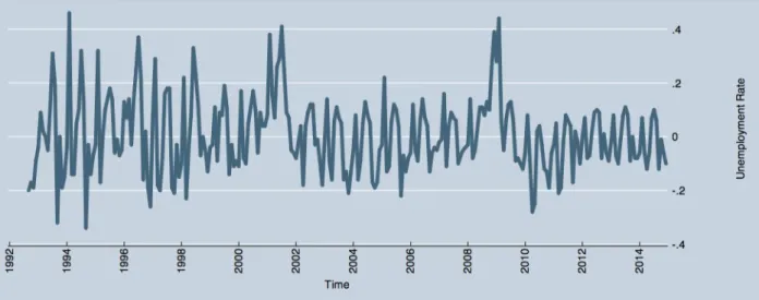
The left hand side of the main empirical model is the percent change in the unemployment rate from the previous period, which in this case is the previous month. I use percent change in the unemployment rate rather than simply using the unemployment rate because vector autoregressive models require relevant variables to be stationary. Figure 7 shows the graph of the percent change in the unemployment rate from the previous month from September 1992 to November 2014. A quick visual analysis of the graph suggests that the percent change in the unemployment rate from the previous month is stationary. This is confirmed in Table 3, which presents the findings of the Dickey-Fuller unit root test.

On the right hand side of the main empirical model, X_{t is the percent change in the}

volume of Taiwan’s trade with China from the previous period. Y_{t is the percent change in the}

volume of Taiwan’s trade with the rest of the world not including China from the previous period. These variables similarly are required to be non-stationary. Figures 8 and 9 show the percent change in total trade with China from the previous month and the percent change in total trade with the rest of the world not including china from the previous month respectively. Both figures seem to suggest that the percent change in trade with China and the percent change in trade with the rest of the world not including China are stationary. The stationarity of these two time series variables is confirmed with the Dickey-Fuller test shown in table 3.

In addition to the vector autoregressive model, I also use the Granger Causality test. A variable X_{t “Granger causes” variable} Y_{t if the lagged values of} X_{t influences variable} Y_t

its own lagged values as well as the other lagged values of the other variables on the right hand side of the of the vector autoregressive model equation as well as the exogenous variables. It tests the null hypothesis that the coefficients on the lagged values of the independent variable in question are jointly 0. If the estimated coefficients are found to be statistically significantly different than zero then we cannot reject that the independent variable in question does not “Granger cause” Y_t.

VI. Results

Now I use the data described in section IV to run the empirical models presented in the previous section to test the relationships between trade and the unemployment rate. First, I use the Johansen Cointegration Test to test if there is a long run relationship between trade with China and the unemployment rate in Taiwan, as in these two variables share a common stochastic drift. The test shows that we cannot reject the null hypothesis that there is no cointegration among the unemployment rate and trade with China. Thus, there is no long run causality between trade with China and the unemployment rate. The test also shows that there is no long run causality between trade with the rest of the world not including China and the unemployment rate.

rest of the world not including China. Column 2 shows the same regression with trade with China as the dependent variable, and column 3 shows the regression with trade with the rest of the world not including China as the dependent variable. The Granger causality and Wald tests show that both growth in trade with China and growth in trade with the world not including China have some predictive power for the percent change in the unemployment rate.

This effect is not the same for trade with the rest of the world. An increase in trade with the rest of the world as a whole not including China decreases the unemployment rate. The theoretical explanation for this outcome as given by the theoretical model presented earlier would be that unemployment decreased in the sector with comparative advantage trading and increased in the sector without comparative advantage. The impact on the unemployment rate overall was an increase in unemployment as a result of increased trade with China suggesting that the magnitude of the increase unemployment in the sector without comparative advantage was greater than the magnitude of the decrease in unemployment in the sector with comparative advantage.

exports to China has a surprising effect as it shows an increase in the unemployment rate as well. The magnitude of this change, 0.005 lagged one period and 0.008 lagged two periods, is much smaller than the magnitude of the effect from imports, but both are statistically significantly different than 0.

The results presented in column 1 of Table 5 also show that an increase in imports with the rest of the world not including China and an increase in exports with the rest of the world not including China have the same impact on the unemployment rate. In the case of the world as a whole though, increased trade in both imports and exports decreases the unemployment rate. The theoretical model does not explain the mechanisms for this outcome. Still, this result is interesting, and holds important policy implications for Taiwan in terms of trade agreements with China. Increased trade in any form, either through imports or exports, both would increase the unemployment rate. However, this is not true for trade with the rest of the world where an increase in both imports and exports would decrease the unemployment rate in Taiwan.

decrease in imports and non-tradable goods. If it is the case that the supply curve for exports to China is more inelastic than the supply curves for non-tradable goods and imports, then the resulting decrease in the unemployment rate from the increase in exports would be overpowered by the increase in unemployment from the necessary increase in the other sectors. The relative elasticity of these supply curves is a possible explanation for why the empirical results show that an increase in exports to China increases the aggregate unemployment rate in Taiwan. A similar explanation of elasticity of supply then, can be used to explain the unexpected result of having an increase in imports from the rest of the world not including China decrease the unemployment rate. The increase in imports from the rest of the world not including China offset by an increase in export sectors and an increase in non-tradable goods sectors would explain the increase decrease in the aggregate unemployment rate if the supply curve for the imports sector was relatively more inelastic than the other sectors.

VII. Conclusion

comparative advantage are the sectors in Taiwan that have the larger increase in magnitude of unemployment. The effect of which overpowers the decreasing unemployment in sectors where Taiwan holds the comparative advantage. Further studies can be conducted on the dynamics of specific sectors trading in Taiwan.

Another important finding of this research is that the effect of imports and exports from China on the unemployment rate in Taiwan is the same. The results show that an increase in both imports and exports from China will increase the unemployment rate. They also show that an increase in both imports and exports from the world overall not including China will decrease the unemployment rate. This could potentially be theoretically explained by differences in supply elasticities in different sectors.

In terms of policy implications, these findings are extremely valuable to ongoing discussions in Taiwan over larger multilateral trade agreements such as the Trans-Pacific Partnership and the Regional Comprehensive Economic Partnership. Trade agreement discussions take into consideration complex social, political as well as economic issues but, if the impact of trade on the aggregate unemployment rate were the deciding factor, given the empirical results of this research, Taiwan would be better advised to sign with the TPP, an agreement with which China has political reasons not to join, rather than the RCEP, which China has taken a leadership role in.

Appendix

Figure 1. Unemployment Rate

Notes: This graph shows the aggregate unemployment rate in Taiwan from August 1992 to November 2014.

Figure 2. Total Trade China

Figure 3. Total Trade with world not including China

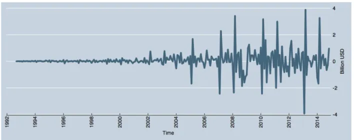
Figure 4. First difference of unemployment rate

Figure 5. First Difference of trade with China

Figure 6. First Difference of total trade with world not including China

Figure 7. Percent change in unemployment rate

Notes: This graph shows the percent change in the unemployment rate in Taiwan between each month from September 1992 to November 2014. The percent change in the unemployment rate is calculated by the difference in the unemployment rate in the current month and the unemployment rate in the previous month divided by the unemployment rate in the previous month.

Figure 9. Percent change in trade with world not including China

Table1. List of Variable Names

Short Name Variable Name Long definition Sources

Unemployment

Rate Unemployment Rate Sample of 20,000 householdsin Taiwan taken monthly. Unemployment rate is calculated by the number of people in the labor force that are unemployed divided by the

number of people in the labor force.

Directorate General of Budget, Accounting and Statistics Percent Change Unemployment Rate

Percent change in the Unemployment

Rate

Percent change in the unemployment rate is calculated by the difference in

the unemployment rate in the current month and the unemployment rate in the previous month divided by the

unemployment rate in the previous month.

Directorate General of Budget, Accounting

and Statistics

Imports China Volume of imports to Taiwan from

China

Total value of goods imported into Taiwan from China in US

dollars

Directorate General of Customs and Administration in the

Ministry of Finance Percent

Change Imports China

Percent change in Imports to Taiwan

from China

Percent change in the imports to Taiwan is calculated by the

difference in the value of imports in the current month and the value of imports in the previous month divided by the

value of imports in the previous month.

Directorate General of Customs and Administration in the

Ministry of Finance

Exports China Volume of exports to China from

Taiwan

Total value of goods exported from Taiwan to China in US

dollars

Directorate General of Customs and Administration in the

Ministry of Finance Percent

Change Exports China

Percent change in exports to China

from Taiwan

Percent change in the exports to China from Taiwan is calculated by the difference in

the value of exports in the

current month and the value of exports in the previous month divided by the value of exports

in the previous month.

Ministry of Finance

Total Trade

China imports and exportsTotal volume of combined between

Taiwan and China

Total trade with China is calculated by the sum of the value of imported goods from

China and value of exported goods to China from Taiwan

in US dollars.

Directorate General of Customs and Administration in the

Ministry of Finance

Percent Change Total

Trade China

Percent change in the total volume of imports and exports

combined between Taiwan and China

Percent change in total trade of Taiwan with China is calculated by the difference in

value of total trade in the current month and the value of

total trade in the previous month divided by the value of

total trade in the previous month.

Directorate General of Customs and Administration in the

Ministry of Finance

Imports World not including

China

Volume of imports to Taiwan from the rest of the world not

including China

Total value of goods imported to Taiwan from the world subtracting the total value of

goods imported to Taiwan from China in US dollars.

Directorate General of Customs and Administration in the

Ministry of Finance Percent

Change Imports World

not including China

Percent change in the volume of imports to Taiwan from the rest of the world not including

China

Percent change in the imports to Taiwan from the world not including China is calculated by the difference in value of imports in the current month and the value of imports in the previous month divided by the value imports in the previous

month.

Directorate General of Customs and Administration in the

Ministry of Finance

Exports World not including

China

Volume of exports from Taiwan to the rest of the world not

including China

Total value of goods exported from Taiwan to the rest of the

world subtracting the total value of goods exported to China from Taiwan in US

dollars.

Directorate General of Customs and Administration in the

Ministry of Finance

Change Exports World

not including China

the volume of exports from Taiwan

to the rest of the world not including

China

to the world not including China from Taiwan is calculated by the difference in

the value of exports in the current month and the value of

exports in the previous month divided by the value of exports

in the previous month.

Customs and Administration in the

Ministry of Finance

Total Trade World not

including China

Total volume of imports and exports

combined between Taiwan and the rest

of the world not including China

Total trade with the world not including china is calculated

by sum of total exports and imports to the whole world subtracted by the sum of total imports and exports to China.

Directorate General of Customs and Administration in the

Ministry of Finance

Percent Change Total

Trade World not including

China

Percent change in total volume of imports and exports

combined between Taiwan and the rest

of the world not including China

Percent change in the total trade with the world not including China is calculated by the difference in the value of total trade in the current month and the value of total

trade in the previous month divided by the value of total

trade in the

Directorate General of Customs and Administration in the

Ministry of Finance

GDP per capita GDP per capita Gross domestic product

divided by total population Directorate General ofBudget, Accounting and Statistics Average Wage Average monthly

earnings Average monthly earningsreported in New Taiwan dollars

Directorate General of Budget, Accounting

and Statistics

MPI Manufacturing

Production Index production using 2011 as theIndex of manufacturing base year

Ministry of Economic Affairs and Statistics

Table 2. Summary Statistics August

1992-December 1995 December 2000January 1996 - December 2005January 2001 - December 2010January 2006 - December 2014January 2011 - All TimePeriods

Observations 41 60 60 60 48 269

Unemployment Rate 1.59 2.79 4.66 4.60 4.19 3.68

(0.26) (0.30) (0.51) (0.83) (0.19) (1.24)

Percent Change

Unemployment Rate 0.58 1.06 0.33 0.36 -0.42 0.40

(11.57) (5.65) (3.35) (2.81) (1.95) (5.63)

Imports China 0.15 0.36 1.03 2.41 3.64 1.51

(0.08) (0.10) (0.47) (0.51) (0.48) (1.33)

Percent Change Imports

China 4.80 3.08 3.79 2.30 2.49 3.22

(18.23) (19.20) (19.46) (16.16) (20.59) (18.61)

Exports China 0.01 0.15 1.97 5.20 6.85 2.84

(0.02) (0.13) (1.29) (1.19) (0.55) (2.80)

Percent Change Exports

China 84.83 5.79 5.67 2.19 0.92 15.94

(237.14) (25.48) (19.68) (17.79) (12.67) (97.04)

Total Trade China 0.17 0.51 3.00 7.61 10.49 4.36

(0.09) (0.22) (1.76) (1.67) (0.95) (4.11)

Percent Change Trade China 5.38 3.35 4.61 2.09 1.24 3.28

(18.02) (17.90) (17.94) (16.31) (14.16) (16.90)

Imports World not including

China 7.08 9.17 10.65 15.72 19.23 12.41

(1.05) (1.38) (2.35) (2.98) (1.32) (4.70)

Percent Change Imports

(10.09) (14.89) (14.18) (14.56) (10.03) (13.17) Exports World not including

China 7.90 10.16 11.25 14.87 18.75 12.62

(1.20) (1.34) (1.43) (2.11) (1.34) (3.91)

Percent Change Exports

World not including China 1.26 1.36 0.85 0.96 0.79 1.04

(11.87) (13.97) (11.30) (11.12) (10.77) (11.82)

Total Trade World not

including China 14.98 19.33 21.89 30.60 37.97 25.03

(2.21) (2.66) (3.71) (5.01) (2.41) (8.56)

Percent Change Total Trade

World not including China 1.11 1.33 0.99 1.21 0.52 1.05

(10.49) (13.75) (12.20) (12.09) (9.78) (11.84)

GDP per capita 3010.88 3464.50 3661.90 4461.85 5423.81 4011.47

(220.40) (195.79) (321.63) (290.75) (226.20) (846.30)

Average Wage 32923.61 39523.58 42289.72 43780.48 46044.21 41247.6₅

(7939.38) (8819.31) (9042.69) (9277.74) (10933.49) (10075.3

5)

MPI 42.24 52.08 64.08 82.38 101.65 68.86

(3.28) (5.82) (8.27) (11.10) (6.69) (21.66)

Table 3. Tests for Stationarity

Variable Test Statistic

Unemployment Rate -2.104

First Difference Unemployment Rate -6.367***

Percent Change Unemployment Rate -13.291***

Total Trade with China -0.255

First Difference Total Trade with China -8.294***

Percent Change Trade with China -25.624***

Total Trade with World Not Including China -1.291

First Difference Total Trade with World Not Including China -8.524*** Percent Change Trade with World Not Including China -26.079***

Imports China 0.127

First Difference Imports China -29.140***

Percent Change Imports China -26.618***

Exports China -0.496

First Difference Exports China -27.000***

Percent Change Exports China -16.755***

Imports World not Including China -2.768*

First Difference Imports World not Including China -26.211*** Percent Change Imports World Not Including China -25.779***

Exports World Not Including China -2.776*

First Difference Exports World Not Including China -26.823*** Percent Change Exports World Not Including China -26.802***

Table 4. Vector Autoregressive Model of Unemployment, Growth in Trade with China, and Growth in Trade with the World

(1) (2) (3)

Dependent Variable:

Percent Change

Unemployment Rate _{Trade with China}Percent Change

Percent Change Trade with World not

including China Percent Change

Unemployment

L1 0.082 0.753*** -0.336***

(0.062) (0.143) (0.098)

L2 -0.080 -0.458*** -0.110

(0.064) (0.147) (0.101)

L3 -0.071 0.487*** 0.291***

(0.065) (0.148) (0.102)

L4 0.001 0.322** 0.089

(0.062) (0.142) (0.098)

Percent Change Trade with China

L1 0.151*** -0.357*** 0.023**

(0.037) (0.084) (0.058)

L2 0.018 -0.041 0.150

(0.039) (0.089) (0.062)

L3 0.009 0.178** 0.094

(0.039) (0.089) (0.062)

L4 0.030 0.051 0.084

(0.037) (0.085) (0.058)

Percent Change Trade with World Not Including China

L1 -0.284*** -0.200* -0.582***

(0.051) (0.118) (0.081)

L2 -0.131 -0.174 -0.311***

(0.060) (0.137) (0.094)

L3 -0.077 -0.131 0.098

(0.060) (0.137) (0.094)

L4 -0.040 -0.193 -0.017

(0.054) (0.124) (0.085)

GDP per capita 0.003** -0.008*** -0.005**

(0.001) (0.003) (0.002)

MPI -0.140*** 0.338*** 0.299***

(0.050) (0.115) (0.079)

Average Wage 0.000 -0.001*** -0.001***

(0.000) (0.000) (0.000)

February 2.779* -25.521*** -11.821***

(1.522) (3.487) (2.401)

March -3.645* 15.487*** 11.523***

(1.919) (4.400) (3.029)

April -2.635 -1.634 2.075

(2.271) (5.205) (3.583)

May 2.407 -12.262** -7.764**

(2.206) (5.056) (3.481)

June 4.348** -22.731*** -14.686**

(2.170) (4.973) (3.424)

July 4.234** -7.995* -7.049**

(2.086) (4.782) (3.292)

August 2.842 -10.589*** -6.896***

(1.986) (4.551) (3.133)

September -4.566** -14.417*** -9.798**

(2.013) (4.615) (3.177)

October -1.407 -17.336*** -7.963***

(1.983) (4.546) (3.130)

November -3.584* -17.340*** -10.195***

(1.992) (4.566) (3.143)

December -4.013** -18.194*** -8.855***

(1.789) (4.100) (2.823)

Table 5. Vector Autoregressive Model of Unemployment and Growth in Imports and Exports

(1) (2) (3) (4) (5)

Dependent Variable: Percent Change Unemployment Rate Percent Change Imports from China Percent Change Exports to China

Percent Change Imports from the World Not

Including China

Percent Change Exports to the World

not Including China Percent Change

Unemployment Rate

L1 0.065 -0.686*** -4.083*** -0.407*** -0.234***

(0.062) (0.152) (1.309) (0.128) (0.090)

L2 -0.026 -0.562*** -5.497*** -0.181 -0.132

(0.064) (0.157) (1.349) (0.132) (0.093)

L3 -0.039 0.521*** -2.031 0.303** 0.282***

(0.063) (0.155) (1.335) (0.131) (0.092)

L4 0.009 0.154 0.011 0.027 -0.027

(0.062) (0.152) (1.311) (0.128) (0.091)

Percent Change Imports from China

L1 0.103*** -0.488*** -0.774 -0.024 -0.011

(0.034) (0.082) (0.710) (0.069) (0.049)

L2 0.002 -0.273*** -0.417 0.022 -0.029

(0.037) (0.090) (0.776) (0.076) (0.054)

L3 -0.001 0.119 -0.538 0.019 -0.028

(0.037) (0.090) (0.775) (0.076) (0.054)

L4 0.004 -0.053 0.258 -0.101 -0.054

Percent Change Exports to China

L1 0.005** -0.003 -0.060 -0.007 -0.003

(0.003) (0.007) (0.057) (0.006) (0.004)

L2 0.008*** 0.001 -0.039 -0.006 -0.001

(0.003) (0.007) (0.056) (0.006) (0.004)

L3 -0.003 0.006 -0.041 -0.002 -0.001

(0.003) (0.007) (0.057) (0.006) (0.004)

L4 -0.003 -0.001 0.418*** -0.005 -0.003

(0.003) (0.007) (0.056) (0.005) (0.004)

Percent Change Imports from the World Not

Including China

L1 -0.064 0.034 -0.274 -0.531*** 0.169***

(0.043) (0.105) (0.907) (0.089) (0.063)

L2 -0.068 0.105 0.293 -0.104 0.273***

(0.052) (0.127) (1.098) (0.107) (0.076)

L3 -0.093** 0.157 0.481 0.225*** 0.275***

(0.052) (0.128) (1.098) (0.108) (0.076)

L4 -0.015 -0.043 0.483 0.086 0.052

Percent Change Exports to the World Not

Including China

L1 -0.198*** 0.038 -1.245 0.005 -0.755***

(0.058) (0.142) (1.227) (0.120) (0.085)

L2 -0.051 -0.040 -1.443 -0.094 -0.491***

(0.074) (0.181) (1.559) (0.153) (0.108)

L3 0.095 -0.171 -1.849 -0.117 -0.135

(0.075) (0.183) (1.574) (0.154) (0.109)

L4 0.016 0.082 -3.247*** 0.093 0.077

(0.059) (0.145) (1.253 (0.123) (0.087)

Exogenous Variables

GDP per capita 0.003** -0.006** 0.026 -0.008*** -0.004**

(0.001) (0.003) (0.026) (0.003) (0.002)

MPI -0.130*** 0.242** -1.828* 0.403*** 0.215***

(0.049) (0.119) (1.024) (0.100) (0.071)

Average Wage 0.000 0.001*** -0.002* -0.001*** -0.001***

February 3.577** -32.853*** -96.867*** -11.787*** -14.686***

(1.518) (3.712) (31.993) (3.131) (2.212)

March -2.104 19.743*** -59.700 6.853* 10.751***

(2.004) (4.901) (42.234) (4.133) (2.920)

April -0.584 -1.975 -13.594 -3.137 1.418

(2.396) (5.860) (50.498) (4.942) (3.491)

May 4.437** -5.890 -38.053 -13.872*** -0.872

(2.231) (5.457) (47.027) (4.602) (3.251)

June 4.544** -20.775*** -17.297 -17.189*** -10.709***

(2.249) (5.500) (47.399) (4.638) (3.277)

July 4.890** -8.531* 3.927 -7.297* -4.193

(2.106) (5.150) (44.383) (4.343) (3.068)

August 3.547* -11.291** -10.601 -11.284*** -4.430

(1.980) (4.843) (41.734) (4.084) (2.885)

September -2.568 -13.167*** -33.714 -15.548*** -7.335**

(1.983) (4.849) (41.792) (4.090) (2.889)

October -0.892 -14.060*** -49.695* -12.443*** -3.354

(1.972) (4.823) (41.565) (4.068) (2.874)

November -2.344 -13.963*** -69.873** -15.637*** -6.241**

(1.968) (4.813) (41.478) (4.059) (2.868)

December -2.794 -15.371*** -73.639** -11.167*** -6.969***

(1.776) (4.345) (37.446) (3.664) (2.589)

Number of Observations 263 263 263 263 263

References

Attanasio O., Goldberg P. K., & Pavcnik N. (2004). Trade Reforms and wage inequality in Colombia. Journal of Development Economics. 331-366.

Davidson C., Matusz S. (2005). Trade and Turnover: Theory and Evidence. Review of

International Economics. 13:5 861-880.

Davidson C., Martin L., & Matusz S. (1999). Trade and search generated unemployment.

Journal of International Economics. 271-299.

Davidsion C., Martin L., & Matusz S. (1988). The structure of Simple Gneral Equilibrium Models with Frictional Unemployment. Journal of Political

Economy. 96:6 1276-1293.

Dutt P., Mitra D., & Ranjan P. (2009). International Trade and Unemployment: Theory and cross-national evidence. Journal of International Economics. 32-44.

Felbermayr G., Prat J., & Schmerer H. (2011). Trade and unemployment: What do the data say?. European Economic Review. 55 741-758.

Feliciano Z. M. (2001). Workers and Trade Liberalization: The Impact of Trade Reforms in Mexico on Wages and Employment. Industrial and Labor Relations Review. 55:1 95-115.

Unemployment: Theory and evidence from India. Journal of Development

Economics. 269-280.

Helpman E., Itskhoki O. (2010). Labour Market Rigidities, Trade and Unemployment.

The Review of Economic Studies. 77:3 1100-1137.

Krugman P. R. (1993). What Do Undergrads Need To Know About Trade?. The

American Economic Review. 23-26.