ISSN: 2322-1666 print/2251-8436 online
A WEIGHTED ALGORITHM TO SOLVE THE CONFORMABLE TIME FRACTIONAL
REACTION-DIFFUSION-CONVECTION PROBLEM A. MOHAMMADPOUR
Abstract. A simple algorithm is applied in this paper to solve the conformable time fractional reaction-diffusion-convection prob-lem (CTFRDCP) with varriable coefficients. The aim of applying this algorithm is to overcome the inability of the differential trans-form method to solve such problems. The differential transtrans-form method is implemented twice. Once with initial condition, again with boundary conditions. A convex combination of two solutions is considered as solution of the problem.
Key Words: Time fractional heat conduction problem, Fractional differential transform method.
2010 Mathematics Subject Classification: Primary: 35R11; Secondary : 35A22.
1. Introduction
The fractional heat equation includes a fractional derivative with re-spect to space and/or time variable. By replacing the first-order time derivative with a fractional derivative of orderα∈(0,1) to the standard heat equation, we have a time fractional heat equation [1]. For example, models that describe heat conduction in materials with non-standard structure, such as porous materials, ploymers and so on, use derivatives of fractional-order [2,3]. Many articles have been written to obtain an-alytical and numerical solutions of fractional heat conduction equation [5,6,7, 8,9]. A method that gives the exact solutions or approximate
Received: 13 November 2017, Accepted: 21 November 2017. Communicated by Ali Taghavi;
∗Address correspondence to A. Mohammadpour; E-mail: [email protected]; c
2018 University of Mohaghegh Ardabili.
solutions by power series, namely, differential transform method (DTM), proposed by Zhou [10] for solving some boundary value problems in or-dinary dierential equations. To solve some PDEs, the 2D DTM was proposed by Chen and Ho [11]. An alternative technique which is simi-lar to DTM and derived from the power series expansion, named reduced differential transform method (RDTM), proposed by Keskin and Otu-ranc [12] to solve linear and nonlinear PDEs. In this paper, by applying the fractional power series expansions where proposed by Abdeljawad [13], the RDTM is adapted to conformable fractional derivative [14] to solve CTFRDCP of the form
(1.1)
∂αu(x, t)
∂tα +a0(x)u(x, t) +a1(x)
∂u(x, t)
∂x +a2(x)
∂2u(x, t)
∂x2 −f(x, t) = 0,
(x, t)∈[0, L]×[0, T],
with the conditions
u(x,0) =φ(x), 0≤x≤L,
(1.2)
u(0, t) =g(t), 0≤t≤T,
(1.3)
ux(0, t) =h(t), 0≤t≤T,
(1.4)
wherea0(x), a1(x), a2(x), f(x, t), φ(x), g(t) andh(t) are given functions
and ∂
αu
∂tα is the conformable time fractional derivative of orderαdefined
in [14].
The arrangement of this paper is in the following plan: In section 2, the conformable fractional derivative is reviewed. In Section 3, the RDTM is given based on the conformable fractional derivative and a weighted algorithm is introduced. Finally, in Section 4, some test problems are solved in order to show the ability and efficiency of the algorithm.
2. The conformable fractional derivative
In this section, some necessary definitions and mathematical prelimi-naries of the conformable fractional derivative required for our work are reviewed.
Definition 2.1. [14] Given a function f : [0,∞) → R. Then, the conformable fractional derivative off of orderα is defined by
Tα(f)(t) = lim ε→0
f(t+εt1−α)−f(t)
for allt >0, α∈(0,1). Iff isα-differentiable in some (0, a), a >0 and limt→0+f(α)(t) exists, then define
f(α)(0) = lim
t→0+f
(α)(t).
Tα(f)(t) satisfies all the properties in the following theorem.
Theorem 2.2. [14]Let α∈(0,1]and f, g be α-differentiable at a point
t >0, then
i. Tα(c1f+c2g)(t) =c1Tα(f)(t) +c2Tα(g)(t).
ii. Tα(tβ) =βtβ−α for allβ ∈R.
iii. Tα(C) = 0 for all constantC.
iv. Tα(f g)(t) =f(t)Tα(g)(t) +g(t)Tα(f)(t).
v. Tα(fg)(t) = g(t)Tα(f)(tg)2−(tf)(t)Tα(g)(t). Specially for certain function we have [14]
1) Tα(sinα1tα) = cosα1tα.
2) Tα(cosα1tα) = sinα1tα.
3) Tα(e
1
αtα) =e
1
αtα.
Theorem 2.3. [13] Assumef is an infinitely α-differentiable function, for some 0 < α ≤ 1 at a neighborhood of a point t0. Then f has the fractional power series expansion:
f(t) = ∞
X
k=0 Tt0
α f (k)
(t0)(t−t0)kα
αkk! , t0< t < t0+R
1
α, R >0.
Here Tt0
α f (k)
(t0) means the application of the conformable fractional derivative k times.
3. Conformable differential transform method
in this section, at first, we review the basic definitions and operations of RDTM which was introduced in [12].
Consider a function of two variables u(x, t) and suppose that it can be represented as product of two single-variable functions, i.e.,u(x, t) =
f(x)g(t). Based on the properties of differential transform [10], function
u(x, t) can be represented as (3.1) u(x, t) =
∞
X
k=0 Fixi
∞
X
j=0
Gjtj =
∞
X
k=0
whereUk(x) is called t-dimensional spectrom function of u(x, t).
Definition 3.1. If functionu(x, t) is analytic and differentiated contin-uosly with respect to timetand spacex in the domain of interest, then let
(3.2) Uk(x) =
1
k!
∂k ∂tku(x, t)
t=0 ,
where the t-dimensional spectrum function Uk(x) is the transformed
function which is called T-function in brief. The differential inverse transform of Uk(x) is defined as follows:
(3.3) u(x, t) =
∞
X
k=0
Uk(x)tk.
Combining (3.2) and (3.3) gives the solution as
(3.4) u(x, t) = ∞
X
k=0
1
k!
∂k ∂tku(x, t)
t=0 tk.
In real applications, by taking to account n-terms of the series (3.4), the functionu(x, t) can be written by
(3.5) u(x, t) = lim
n→+∞un(x, t) =n→lim+∞
n X
k=0
Uk(x)tk.
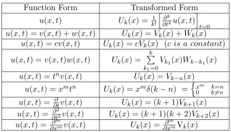
The fundamental operations of reduced differential transform that can be deduced from Eqs. (3.2) and (3.3) are listed in Table 1.
Now, considering Theorem2.3and the fractional power series expansion, we can construct CRDTM, which is based on the conformable fractional derivative.
Definition 3.2. Suppose that u(x, t) be an analytic function that sat-isfies the conditions of Theorem2.3with respect to variabletatt0 = 0. Define
(3.6) Uk(x) =
1
αkk! h∂kα
∂tkαu(x, t) i
t=0,
whereα is order of conformable derivative andUk(x) is the transformed
Table 1. Some basic reduced differential transformations.
Function Form Transformed Form
u(x, t) Uk(x) = k1! h
∂k ∂tku(x, t)
i t=0 u(x, t) =v(x, t) +w(x, t) Uk(x) =Vk(x) +Wk(x)
u(x, t) =cv(x, t) Uk(x) =cVk(x) (c is a constant) u(x, t) =v(x, t)w(x, t) Uk(x) =
k P k1=0
Vk1(x)Wk−k1(x)
u(x, t) =tnv(x, t) U
k(x) =Vk−n(x) u(x, t) =xmtn Uk(x) =xmδ(k−n) =
n
xm k=n
0 k6=n u(x, t) = ∂t∂v(x, t) Uk(x) = (k+ 1)Vk+1(x) u(x, t) = ∂t∂22v(x, t) Uk(x) = (k+ 1)(k+ 2)Vk+2(x) u(x, t) = ∂x∂mmv(x, t) Uk(x) = ∂
m ∂xmVk(x)
Definition 3.3. Let Uk(x) be the transform ofu(x, t) with respect to t, the differential inverse transform ofUk(x) is defined as
(3.7) u(x, t) = ∞
X
k=0
Uk(x)tkα=
∞
X
k=0 h∂kα
∂tkαu(x, t) i
t=0t kα.
All properties of the CRDTM are similar to those in Table 1. For instance, the following theorem is proved.
Theorem 3.4. If u(x, t) = ∂
αv(x, t)
∂tα , then Uk(x) =α(k+ 1)Vk+1(x)
Proof. From Definition3.2we have
Uk(x) =
1
αkk![ ∂kα
∂tkαu(x, t)]t=0=
1
αkk![ ∂kα ∂tkα
∂α ∂tαv(x, t)
]t=0
= 1
αkk![
∂(k+1)α
∂t(k+1)αv(x, t)]t=0 =α(k+ 1)
1
αk+1(k+ 1)![
∂(k+1)α
∂t(k+1)αv(x, t)]t=0
=α(k+ 1)Vk+1(x)
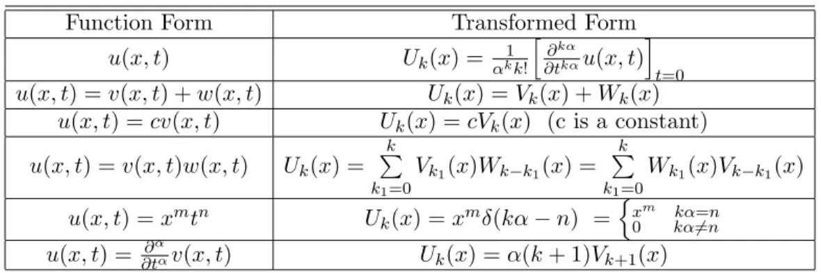
Now, a weighted method according to the CRDTM will be presented to solve the problem (1.1)-(1.4). It is done in two step. At the first step, considering Theorem 3.4 and Table 2, the transformation of Eq.(1.1)
Table 2. Some basic properties of CRDTM.
Function Form Transformed Form
u(x, t) Uk(x) = αk1k!
h ∂kα ∂tkαu(x, t)
i t=0 u(x, t) =v(x, t) +w(x, t) Uk(x) =Vk(x) +Wk(x)
u(x, t) =cv(x, t) Uk(x) =cVk(x) (c is a constant) u(x, t) =v(x, t)w(x, t) Uk(x) =
k P k1=0
Vk1(x)Wk−k1(x) =
k P k1=0
Wk1(x)Vk−k1(x)
u(x, t) =xmtn Uk(x) =xmδ(kα−n) = n
xm kα=n
0 kα6=n u(x, t) = ∂t∂ααv(x, t) Uk(x) =α(k+ 1)Vk+1(x)
and initial condition(1.2) with respect tot we have (3.8)
α(k+1)Uk+1(x)+a0(x)Uk(x)+a1(x) ∂
∂xUk(x)+a2(x) ∂2
∂x2Uk(x)−Fk(x) = 0,
whereFk(x) is transformation off(x, t). By substituting of theU0(x) = φ(x) as transformation of (1.2) into (3.8), the approximate solution (3.9) uˆn(x, t) =
n X
k=0
Uk(x)tkα.
will be obtained.
At the second step, we seek the series solution of the Eq.(1.1) according to boundary conditions (1.3) and (1.4). Again considering Theorem3.4 and Table 1, take differential transform of Eq.(1.1) with respect to x
and get (3.10)
∂α
∂tαUk(t) + k P k1=0
Uk1(t)A0(k−k1)(x) +
k P k1=0
k1(k1+ 1)Uk1+1(t)A1(k−k1)(x)+
k P k1=0
(k1+ 1)(k1+ 2)Uk1+2(t)A2(k−k1)(x)−Fk(t) = 0
Where Ui(t), Ai(x), and Fi(t) are transformation of u(x, t), ai(x), i =
0,1,2 andf(x, t) with respect tox. From the boundary conditions (1.3) and (1.4), we have
and
(3.12) U1(t) =h(t).
Substituting (3.11) and (3.12) into (3.10), we can get the successive values of Ur(t). In result, the series solution
(3.13) uˇn(x, t) = n X
r=0
Ur(t)xr.
will be obtained. An approximate solution to problem (1.1)-(1.4) is considered as the following weighted combination.
(3.14) un(x, t) =λuˆn(x, t) + (1−λ)ˇun(x, t),
where λ is a constant on the interval [0,1]. For determining the best value of λfor each n, we use the idea presented in [15].
Theorem 3.5. Suppose that φ(x) ∈ L2[(0, L)], g(t), h(t) ∈ L2[(0, T)]
and k.k denotes the L2−norm. Let
λ1 =kuˆn(0, t)−g(t)k, λ2 =k∂uˆn
∂x (0, t)−h(t)k, λ3 =kuˇn(x,0)−φ(x)k.
Then the best value for λin (3.14) is
λ= λ
2 3
λ21+λ22+λ23, n≥0.
Proof. refer to [15].
4. Illustrative examples
To show the applicability of the CRDTM, some examples will be pre-sented. We usenterms in evaluating the approximate solution un(x, t).
Example 4.1. As the first example consider (4.1) ∂
αu(x, t) ∂tα −
∂u(x, t)
∂x −x
∂2u(x, t)
∂x2 +4x−1 = 0, (x, t)∈[0,1]×[0,1],
with the conditions
u(x,0) =x2, 0≤x≤1,
(4.2)
u(0, t) =ux(0, t) =
1
αt
α, 0≤t≤1.
Using Theorem 3.4 and Table 2, transformation of the Eq.(4.1) with respect totbecomes
(4.4) α(k+ 1)Uk+1(x)− ∂
∂xUk(x)−x ∂2
∂x2Uk(x) + (4x−1)δ(kα) = 0.
SubstitutingU0(x) =x2 as transformation of the initial condition (4.2) into recurrence relation (4.1) gives the next Uk(x), k≥1 as
U1(x) =
1
α, Uk(x) = 0, k= 2,3,· · ·
From (3.9), the inverse differential transform ofUk(x) gives:
ˆ
un(x, t) = n X
k=0
Uk(x)tkα =x2+
1
αt α
Now, use the basic properties of the reduced differential transform of Ta-ble 1 with respect tox. Transformation of the Eq.(4.1) and the boundary conditions (4.3) to x becomes
(4.5) ∂
α
∂tαUk(t)−(k+ 1)Uk+1(t)−k(k+ 1)Uk+1(t) + 4δ(k−1)−δ(k) = 0
and
(4.6) U0(t) =U1(t) = 1
αt
α.
To take the nextUk(x), k≥2, replace (4.6) into recurrence relation (4.5)
and give
U2(t) =5
2α, Uk(t) = 0, k= 3,4,· · · . From (3.13) the inverse differential transform of Uk(x) gives:
ˇ
un(x, t) = n X
k=0
Uk(x)xk=
1
αt
α+ 1
αt
αx+5 2αx
2.
Asλ= 1 for n≥8, the Eqs. (3.14) and (3.5) give lim
n→+∞ un(x, t) = ˆun(x, t)
=x2+ 1
αt α,
which is the exact solution of the problem.
Example 4.2. Consider the following problem (4.7)
∂αu(x, t)
∂tα −
∂2u(x, t)
∂x2 −
∂u(x, t)
∂x −u(x, t)+e
1
αt α
with the conditions
u(x,0) =x, 0≤x≤1,
(4.8)
u(0, t) = 0, ux(0, t) =e
1
αt α
, 0≤t≤1.
(4.9)
Being in a similar way with the first example, we apply the Theorem 3.4and Table 2 to Eq.(4.7) and achieve the following relation.
(4.10) α(k+ 1)Uk+1(x) = ∂2
∂x2Uk(x) + ∂
∂xUk(x) +Uk(x)−
1
αkk!.
Substituting the initial condition (4.8),i.e. U0(x) =xinto relation (4.10) we have
U1(x) =
1
αx, U2(x) =
1
2α2x, U3(x) =
1
6α3x, · · ·, Uk(x) =
1
k!αkx.
Therefore, we obtain the approximate solution ˆ
un(x, t) = n X
k=0
Uk(x)tkα =x+
1
αxt α+ 1
2α2xt 2α+ 1
6α3xt
3α+· · ·+ 1 n!αnxt
nα.
On the other side, using the basic properties of the reduced differential transform of Table 1 with respect tox, for the Eq.(4.7) and the boundary conditions (4.9) we take the relation
∂α
∂tαUk(t)−(k+ 1)(k+ 2)Uk+2(t)−(k+ 1)Uk+1(t)−Uk(t) +e
1
αt α
δ(k) = 0,
or (4.11)
(k+ 1)(k+ 2)Uk+2(t) = (k+ 1)Uk+1(t) +Uk(t)− ∂α
∂tαUk(t)−e
1
αt α
δ(k) and
(4.12) U0(t) = 0, U1(t) =e
1
αt α
.
Replace (4.12) into (4.11) and obtain Uk(t) = 0, k≥2. So, we take the
solution of the problem (4.7) with boundary conditions (4.9) as ˇ
un(x, t) = n P k=0
Ukxk= 0 +e
1
αt α
x+ 0 =xeα1t α
.
Here,λ= 0 for n≥5. Hence, by Eqs. (3.14) and (3.5), lim
n→+∞ un(x, t) = ˇun(x, t)
=xeα1t α
.
Example 4.3. The function u(x, t) = sin(x+ α1tα) is the exact solution of the problem
(4.13) ∂
αu(x, t) ∂tα +x(
∂2u(x, t) ∂x2 +
∂u(x, t)
∂x )−cos(x+
1
αt
α) = 0,
with the initial and boundary conditions
u(x,0) = sinx, 0≤x≤ 1
2, (4.14)
u(0, t) = sin ( 1
αt α), u
x(0, t) = cos (
1
αt
α) 0≤t≤ 1
2. (4.15)
For this problem, we compute an approximate solution and compare it with the exact solution.
The transformed form of the Eqs. (4.13) and (4.14) with respect to t
becomes
(4.16) (k+1)Uk+1(x)+x ∂2
∂x2Uk(x)+xUk(x)−
1
αkk!cos( kπ
2 + 1
αt α) = 0.
SubstitutingU0(x) = sinx, the transformed form of the initial condition
(4.14), into the relation (4.16) gives (4.17)
U1(x) = α1 cos(x), U3(x) =−6α13cos(x), U5(x) = 1201α5 cos(x),· · ·,
U2k+1(x) = (−1)
k
(2k+1)!α2k+1cos(x)
U2(x) =−2α12 sin(x), U4(x) = 241α4sin(x), U6(x) =−7201α6 sin(x),· · ·,
U2k(x) = (
−1)k
(2k)!α2ksin(x)
Now, we take the differential transformation of the Eq.(4.13) with re-spect tox. Again we apply the properties of differential transformation in Table 1 and obtain
∂α
∂tαUk(t) +k(k+ 1)Uk+1(t) +Uk−1(t)−
1
k!cos(
kπ
2 + 1
αt
α) = 0,
or (4.18)
Uk+1(t) =
1
k(k+ 1)
−∂
α
∂tαUk(t)−Uk−1(t) +Uk(t) +
1
k!cos(
kπ 2 + 1 αt α) .
SubstitutingU0(t) = sin (α1tα) and U1(t) = cos (1αtα), the transformed form of the boundary conditions (4.15), into relation (4.18) gives the
next term of Uk(t), k≥2 as
(4.19)
U2(x) =−12sin(α1tα), U4(x) = 1445 sin(α1tα), U6(x) =−4320041 sin(α1tα),· · · U3(x) =−121 cos(1αtα), U5(x) = 7201 cos(α1tα), U7(x) = 567001 cos(α1tα),· · · .
Therefore, the Eqs. (4.17) and (4.19), give the approximate solution by (3.9), (3.13) and (3.14).
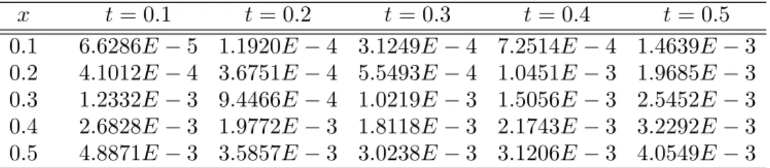
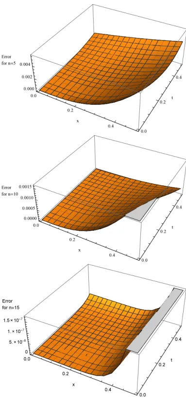
According to the Theorem 3.5, we get λ = 0.449,0.594,0.663 For n = 5,10,15 respectively. The relative errors of the approximation, have been given in Table 3, Table 4 and Table 5. Also, Figure 1 indicates the function error for{(x, t)|0≤x≤ 1
2,0≤t≤ 1 2}.
Table 3. The relative error of the computed
approxi-mate solution of the Example 3 byn= 5.
x t= 0.1 t= 0.2 t= 0.3 t= 0.4 t= 0.5 0.1 6.6286E−5 1.1920E−4 3.1249E−4 7.2514E−4 1.4639E−3 0.2 4.1012E−4 3.6751E−4 5.5493E−4 1.0451E−3 1.9685E−3 0.3 1.2332E−3 9.4466E−4 1.0219E−3 1.5056E−3 2.5452E−3 0.4 2.6828E−3 1.9772E−3 1.8118E−3 2.1743E−3 3.2292E−3 0.5 4.8871E−3 3.5857E−3 3.0238E−3 3.1206E−3 4.0549E−3
Table 4. The relative error of the computed
approxi-mate solution of the Example 3 byn= 10.
x t= 0.1 t= 0.2 t= 0.3 t= 0.4 t= 0.5 0.1 2.4524E−5 1.5120E−5 9.9538E−6 6.3766E−6 3.8580E−6 0.2 1.7586E−4 1.1260E−4 7.5169E−5 4.7064E−5 2.3597E−5 0.3 5.4093E−4 3.5778E−4 2.4264E−4 1.5235E−4 7.3519E−5 0.4 1.1849E−3 8.0621E−4 5.5490E−4 3.4989E−4 1.6451E−4 0.5 2.1641E−3 1.5105E−3 1.0541E−3 0.6740E−4 3.0572E−4
Figure 1. The error function of the approximate solution of the example 3 forn= 5,10,15.
Table 5. The relative error of the computed
approxi-mate solution of the Example 3 byn= 15.
x t= 0.1 t= 0.2 t= 0.3 t= 0.4 t= 0.5 0.1 5.2963E−8 4.8109E−8 6.1769E−9 2.0888E−10 3.3379E−10 0.2 4.7110E−8 4.2793E−8 5.4943E−8 1.8580E−10 2.9323E−10 0.3 4.1394E−7 3.7599E−8 4.8276E−8 1.6325E−9 2.5846E−9 0.4 3.5883E−7 3.2594E−7 4.1849E−7 1.4151E−8 2.2515E−9 0.5 3.0648E−7 2.7839E−7 3.5744E−7 1.2087E−8 1.9105E−8
5. Conclusion
In this study, the time fractional reaction-diffusion-convection prob-lem with varriable coefficients has been solved. The time derivative has been considered the conformable fractional derivative. Reduced differ-ential transform method has been adapted to conformable fractional derivative, then has been applied to obtain two approximate solution. One of them with respect to time variable t by initial condition and another, with respect to space variable x by boundary conditions. A convex combination of two solution has been introduced as the approxi-mate solution of the problem. The given examples, have shown that the proposed method yield good results.
References
[1] Y.Z. Povstenko, Fractional heat conduction equation and associated thermal stress, J. Therm. Stresses,28(2005) 83-102.
[2] D. Sierociuk, A. Dzielinski, G. Sarwas, I. Petras, I. Podlubny, T. Skovranek,
Modelling heat transfer in heterogeneous media using fractional calculus, Philos. Trans. R. Soc. A,371(2013) 1-10.
[3] Y. Zhou,Basic Theory of Fractional Differential Equations, World Scientic, 2014. [4] F. Mainardi, Y. Luchko, G. Pagnini,The fundamental solution of the space-time
fractional diffusion equation, Fract. Calc. Appl. Anal.,4(2) (2001) 153-192. [5] P. Zhuang, F. Liu,Implicit difference approximation for the time fractional
dif-fusion equation, J. Appl. Math. Comput.,22(3) (2006) 87-99.
[6] S. Momani, Z. Odibat, Numerical solutions of the space-time fractional advec-tiondispersion equation, Numer. Methods Partial Differ. Equ., 24 (6) (2008) 1416-1429.
[7] A. Taghavi, A. Babaei, A. Mohammadpour,A coupled method for solving a class of time fractional convection-diffusion equations with variable coefficients, Comp. Math. Modeling,28(1) (2017).
[8] A. babaei, A new accurate approach to solve the Cauchy problem of the Kolmogorov-PetrovskiiPiskunov equations, Int. J. App. Comp. Math., (2017) 1-14.
[9] A. babaei, A. Mohammadpour, Solving an inverse heat conduction problem by reduced differential transform method, New Trends in Mathematical Sciences,3
(3) (2015) 65-70.
[10] J. K. Zhou, Differential transform and its applications for electrical circuits, Huazhong University Press, Wuhan, China, 1986.
[11] C.K. Chen, S.H. Ho,Solving partial dierential equations by two-dimesional dier-ential transform method, Appl. Math. and Comput.,106(1999) 171-179. [12] Y. Keskin, G. Oturanc,Reduced Differential Transform Method for partial
dif-ferential equations, Inter. Jour. Nonl. Scie. Num. Simu.,6(10) (2009) 741-749. [13] T. Abdeljawad, On conformable fractional calculus, J. Comput. Appl. Math.,
279(2015) 57-66.
[14] R. Khalil, M. Al Horani, A. Yousef, M. Sababheh,A new definition of fractional derivative, J. Comput. Appl. Math.264(2014) 65-70.
[15] Shidfar, A., Garshasbi, M.,A weighted algorithm based on Adomian decomposi-tion method for solving an special class of evoludecomposi-tion equadecomposi-tions, Commun. Non-linear Sci. Numer. Simulat.,14(2009) 1146-1151.
A. Mohammadpour
Department of Mathematics, Babol branch, Islamic Azad University, Babol, Iran.