Vol 6, No 9 (2015)

(1)

Available online throug

ISSN 2229 – 5046

AN ORDERING POLICY WITH VARYING DEMAND FOR DETERIORATING ITEMS

T. Mohanreddy*

1

_{, K. Srinivasa Rao}

2

_{, C. T. Suryanarayana Chari}

3

1

_{Department of Mathematics, St. Joseph’s Degree college, Kurnool.}

2

_{Professor, Department OR & SQC, Rayalaseema University.}

3

_{Dept. of Mathematics, Silverjubliee College, Kurnool, (A.P.) – 518004.}

(Received On: 19-08-15; Revised & Accepted On: 16-09-15)

ABSTRACT

I

n this paper we have consider an order level inventory model with varying demand for deteriorating items. Here the demand is initially constant and after some period of time the demand increases exponentially due to maximum shortages we also considered deteriorating items and price breaks allowing shortages.

Key words: Order level inventory, Exponential increasing demand, deteriorating items, price breaks.

INTRODUCTION

Several researchers have attempted to obtain optimal ordering quantity for deteriorating items. In real word problems several factors will influence for obtaining optimal ordering quantitySeveral Researchers attempted inventory models for price breaks for example Abad [1] has attempted to determined selling price and lot size for retailer when he is given all units discounts, further Arcelus et al. [2] considered the forward buying policies of an inventory model with deteriorating items and temporary price discounts. Fazal et al. [3] also considered the classical quanity discount model from the variety of EOQ models basically presented by Harris [4] Hwang et al. [5] considered an EOQ model with quantity discouts for both purchasing price and Freight cost. Matsuyama et al. [6] portrayed EOQ models with price discounts. Rubin et al. [7] also attempted to obtain EOQ with price discounts. A comparpison with JIT (Vs) EOQ with price discounts presented by Chaudhuri et al. [8].

In the recent literature of Inventory models, several researchers considered deterioration of Items. Deterioration place a major role for stocking of goods even in supply chain management, in this area an attempt is made by Rau et al. [9] by considering deterioration of Items in supply chain management. Inventory model for determining items by allowing shortages is considered by Dye et al. [10] chung et al. [11] also attempted in determining an EOQ model with deteriorating items under varying demand. The delay in payments for deteriorating items in the context of EOQ models is discussed by skouri et al. [12]. The deterioration of Inventory Items are classified into three categories by Ghare and Schrader [13]. These three categories are direct spoilage, physical depletion and deliration. Direct spoilage means breakage of Items which cannot be used further. where as deterioration refers to the slow but gradual loss of qualitative properties of the items in a phased manner.

2. NOTATIONS

q(t) - Inventory level at time ‘t’

s=q(0) = Stock level at the beginning of each ccycle after fulfilling back orders

S0 = q (T0) = Stock level below which the demand rate is constant. It is an external variable beyond the control of the decision maker

Q = Stock level at the begininning the amount of shortages. D = Constant demand rate

T0 = Time unitl stock level reaches S0 T1 = Time unitl shortage begins T = Length of the cycle time

Corresponding Author: T. Mohanreddy*

1

(2)

θ

= Deterioration rate, fraction of the on hand inventory

C2 = Shortage cost per unit per unit time C3 = The ordering cost of Inventory

Pi = The unit cost of item in fi-1< S <fi, where i = 1 to N and = f0<f1<f2 ...fN PN = The unit cost of item in fN<S

h = Inventory holding cost per item per unit time U = The unit selling price of deteriorated items

3. ASSUMPTIONS

The following assumptions are considered

i) Shortages are allowed and are fully back logged ii) The replenishment is Instantaneous.

iii) Deteriorated items are sold at a low price at the end of the stocks

iv) Two - Component exponential demand rate is considered i.e. demand depends on the inventory as well as on the fixed customers

v) price breaks are considered here i.e. the unit purchase price is discounted with the increasing ordering quantity.

4. FORMULATION OF THE MODEL

In real word, initially the demand of the product may not be high. To increase the demand of the product, the pruaent management may implement several advertising strategies. Hence demand may vary, that means initially demand is constant, when the product is launched and it may suddenly increases. Here we assume that upto certain period a constant demand and latter exponential increasing demand.

The inventory level will be depleted at a rate of during the period (0, T0) is ‘D’. During the period (T0, T1) the Inventory level will be depleted at a exponential rate

The inventory falls to zero level at time t = T1, shortages are than allowed for replenishment up to time t = T. Therefore, for a deteriortionrate the instantaneous inventory level will satisty the following differential equation.

will the satisfy the following equation

with the boundary conditions are

t

aeα

D q dt dq_+θ ₌₋

) 1 ( 0<t<T₀→

) 2 ( ) 0

( =S→

q

) 3 ( ) (T₀ =S₀→ q

t

ae q dt

dq₊_θ ₌₋ α

( )

4

1 0<t<T →

(3)

An Ordering Policy with Varying Demand for Deteriorating items / IJMA- 6(9), Sept.-2015.

With the boundary conditions

where

With the boundary Conditions are

The solution of th e equation (1) is

By using boundary condition and

Substituting (11) in (10) we get

The solution of (12) with boundary condition t = T0 and q(t1) = 0

The solution of the equation (4) with the boundary condition is

By using the boundary condition q(T0) = S0

T0< t < T1

The boundary condition from (6) is

( )

T₀ =S₀→(5)

q

( )

T₁ =0→(6)

q

t

ae dt dq₌₋ α

( )

7

1<t<T→

T

( )

T₁ =0→

( )

8

q

( )

T =−

(

Q−S

) ( )

→9

q

1

. . .

.IF QIF K

Y =∫ +

1

.e De K

Q θt₌_∫₋ θt₊

( )

t.e D e dt K1

q θt₌₋ _∫ θt ₊

( )

1→

( )

10

  

 

+ − = −

K e D e t q

t t

θ

θ θ

( )

0 S,

q = _t₌₀

( )

11

1= +_θ →

D S K

( )

→

( )

12

     + + −

= −

θ θ θ

D S e D t

q t

0

0<t<T

0

0 =

     + +

− −

θ θ θ

D S e

D T

θ θ

θ D D

S

e T _₌

     +

− 0

     

+ = −

θ θ

S D

D T0 log

( )

13 log

1

0 →

    

+ −

=

θ θ D S

D T

1 0 t T

T < <

2

. . .

.IF QIF K

Y =∫ +

( )

te ae .e K2

q θt ₌_∫₋ αt θt₊

( )

₊ + 2 →

( )

14

−

= t −t

e K e a t

q α θ

θ α

0 0

2 0

T T

e K e a

S α θ

θ α

−

+ + − =

( )

15 0 0

0

2 →

  

 

+ +

= T T

e a S e

K θ α

θ α

t T T

T

e e a S e e a

S α θ α θ

θ α θ

α

−

   

 

   

 

+ + +

+ −

= 0 0 0

0 0

( )

_{( )}

16 )

( 0 0 0

0  →

  

 

+ + + + −

= T T − t−T

e e a S e a t

q α α θ

θ α θ

α

( )

T1 =0

(4)

It gives

The solution of equation (7) with the boundary condition

q

( )

T

₁

=

0

is

The boundary condition

Here the total variable cost is consist of fixed cost, holding cost, shortage cost, purchased cost minus the selling price of the deteriorated items. They are sumed up after evaluating the above cost individually

The ordering cost OC = C3

The holding Cost

The deteriorated items =

The selling price of deteriorated items

The shortage cost SHC for a cycle is

The purchase cost PC fer a quantity of amount is

The total cost function

(

)

_{( )}

17 log 1 0 0

1 →

     + + + + + = θ α θ α θ α a S T T

(

)

_{( )}

18 log 1 log 1 0

1 →

     + + + + +       + − = θ α θ α θ α θ θ a S S D D T

( )

_t _a_e ( )

_{( )(}

_T _t _T

₎

q =− . t−T1 →19 1< <

α

( ) (

T Q S

)

gives q =− −

( )

20

1 → − + = _t ae S Q T T _α

(

)

_{( )}

21 log 1 log

1 0 _+ − →

     + + + + +       + − = _t ae S Q a S S D D T _α θ α θ α θ α θ θ

( )

HC h q

( )

tdt h q

( )

tdt

T T T 1 0 0 0 ∫ + ∫ = ( )                   + + + + − ∫ +             + + − ∫ = − − − dt e e a S e a dt D S e D

h T T tT

T T t T 0 0 0 1 0 0 0 0 θ α α θ θ α θ α θ θ ( )

( )

22 1

1 1 0

0 0

0

0 →

                      −       + + −       − + − +             +       + − − = − − − θ θ θ α α α θ α θ θ θ θ θ α α α

θ T T

T T T T e e a S e e a e D S T D h HC

( )

      ∫ + ∫

− Ddt ae dt

q t T T T α 1 0 0 0 0

( )

23

0

0 →

            − + − = α α α

αT T

e e a DT S

( )

24

0

0 →

                    − + − = α α α

αT T

e e a DT S U DP

( )

tdt q C SHC T T1 2∫ − =

(

Q S

)

dt C T T − − ∫ − = 1 2

(

)

_{( )}

25 2 2 2 → − = D S Q C SHC

(

fi S fi

)

S −1< <

( )

26

→ =PS PC _i DP PC SHC HC OC

TVC= + + + −

( )                     −       + + −       − + − +             +       + − − + = − − − θ θ θ α α α α θ α θ θ θ θ θ α α θ 1

1 1 0

0 0 0 0 0 3 T T T T T e e a S T e e a e D S T D h C

(

)

_{( )}

27 2 0 0 0 2

2 →

                    − + − − + − + α α α

αT T

(5)

The selling price SR fer a quantity of non- deteriorated amount is

The total profit function TP is defined as TP(S,Q) = SR-TVC

=

The total profit per unit time

(

)

(

)

S

T

Q

S

TO

Q

S

TPU

,

=

,

−

Here the profit function (30) is to be maximized

NUMERICAL EXAMPLE AND SENSITIVITY ANALLYSIS

The set up cost

( )

C

₃ -8350 / order

The demand

( )

D

- 400/ month

The shortage cost

( )

C

₂ 0.5/ unit

The holiday cost per unit (h) 12

The selling price of deteriorated items (u) = 15

Quantity Purchase cost Selling Price

500

0 <

S

<

40 50

1000

500 <

S

<

30 38

2000

1000

<

S

<

28 35

S

<

2000

20 26

The Problem is solved by genetic algorithm and is given in appendix. The solutions for different parametric values of

θ

_{, a, b, c and so are given in Table 1 to 4}

( )

28

0

0 →

            − − + − = α α α

αT T

i e e a DT S S V SR               − − + − = α α α α 0 0 0 T T i e e a DT S S V

SR ( )

                        −       + + −       − + − +             +       + − − +

− _θ _θ _θ−θ _θ1 _α _θ _αα _αα _α _θ α −θ_θ1−0 _θ1

0 0 0 0 0 3 T T T T T T _e e a S e e a e D S T D h C

(

)

                          − + − − + − + α α α α 0 0 0 2 2 2 T T i e e a DT S U S P D S Q C

(

)

          − + +       +       ₊ + + − − − α α θ α θ θ θ θ α α

θ0 ₁ 0

0 0 3 T T T i i e e ha e D S h T hD C S P V ( )

₍

₎

                      − + − + − +       −       + + + − − α α θ θ θ α α α θ

α 1 0 0

0 0 0 2 2 0 2

1 T T

T T

T e e

a DT S U D S Q C e e a S h                         − + − − α α α α 0 0 0 T T i e e a DT S V

(

)

          − + +       +       ₊ + + − − = − α α θ α θ θ θ θ α α

θ0 ₁ 0

0 0 3 T T T i i e e ha e D S h T hD C S P V TP ( )

₍

) (

)

( )

29

2 1 0 0 1 0 0 0 2 2

0 →

                      − + − − + − +       −       + + + − − α α θ θ θ α α α θ

α T T

i T

T

T e e

a DT S V U D S Q C e e a S h

(

)

          − + +       +       ₊ + + − − = − α α θ α θ θ θ θ α α

θ0 ₁ 0

1 0 0 3 T T T i i e e ha e D S h T hD C S P V T TPU ( )

₍

) (

)

( )

30

2 1 0 0 1 0 0 0 2 2

0 _→

                      − + − − + − +       −       + + + − − α α θ θ θ α α α θ

α T T

i T

T

T e e

(6)

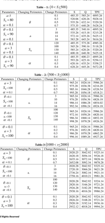
Table – 1:

(

0 < <

S

500 )

Parameters Changing Perimeters Change Perimeters S Q TPU .a=3

80

0

=

S

1 .

0 =

α

θ

0.1 0.3 0.5 0.7

485.35 520.06 535.26 575.35

585.24 620.26 632.14 640.28

4895.26 5028.16 5320.26 5428.24

1 .

0 =

θ

90

0

=

S

1 .

0 =

α

.a

3 10 14 16

485.35 535.26 572.14 583.28

540.16 615.18 635.26 645.24

4895.26 5215.28 5425.12 5616.26

1 .

0 =

θ

3 =

a

1 .

0 =

α

S

0

120 100 130 140

485.35 565.26 585.24 600.18

575.28 590.16 620.26 640.38

4985.26 5118.28 5320.26 5425.18

1 .

0 =

θ

3 =

a

90

0

=

S

α

0.1 0.2 0.3 0.4

485.35 593.26 620.16 628.24

600.23 625.16 635.24 645.26

4895.26 5256.12 5358.23 5472.28

Table – 2:

(

500 <

S

<

1000

)

Parameters Changing Perimeters Change Perimeters S Q TPU

3 =

a

0

S

=100

=

α

0.1

θ

0.1 0.3 0.5 0.7

965.24 975.28 985.16 995.28

1026.16 1036.38 1046.28 1056.18

5986.26 6216.20 6326.54 6518.21

θ

=0.1

0

S

=100

α

=0.1

a.

3 10 14 16

965.24 976.28 986.14 992.34

1026.16 1056.36 1086.28 1096.24

5986.26 6826.18 6854.02 6924.18

θ

=0.1 a.=100

α

=0.1

S

0

100 120 130 140

965.24 972.16 986.34 998.28

1026.16 1058.26 1068.14 1078.28

5986.26 6820.16 6852.18 6926.26

1 .

0 =

θ

3 =

a

100

0

=

S

α

0.1 0.2 0.3 0.4

965.24 976.26 986.28 996.16

1026.16 1052.28 1070.28 1089.26

5986.26 6820.16 6862.28 6927.26

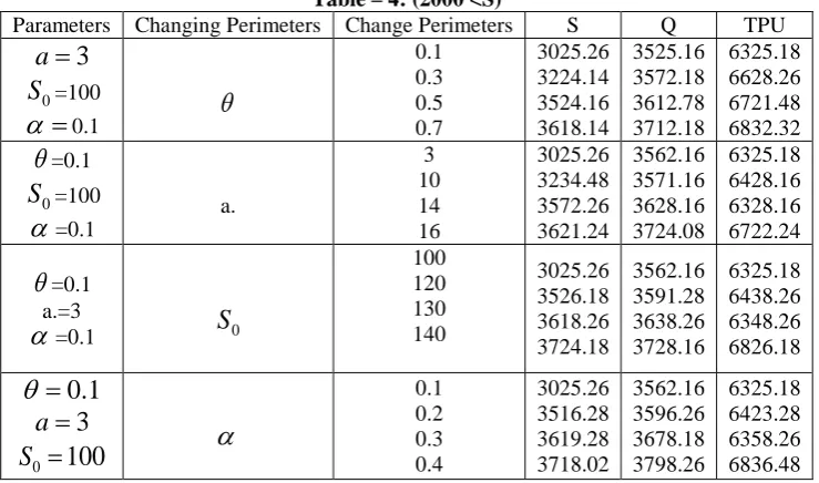
Table-3:

(

1000

<

s

<

2000

)

3 =

a

0

S

=100

=

α

0.1

θ

0.1 0.3 0.5 0.7

2020.25 2620.18 2635.16 2652.08

3042.92 3056.16 3072.16 3092.34

9325.14 9526.18 9828.16 9878.28

θ

=0.1

0

S

=100

α

=0.1

a.

3 10 14 16

2020.28 2720.18 2736.24 2758.16

3042.92 3066.26 3082.16 4010.21

9325.14 9621.28 9921.14 9981.26

θ

=0.1 a.=3

α

=0.1

S

0

100 120 130 140

2020.28 2820.16 2926.28 2938.16

3042.92 3166.26 3182.28 4016.26

9324.14 9721.24 9936.16 9986.24

1 .

0 =

θ

3 =

a

100

0

=

S

α

0.1 0.2 0.3 0.4

2020.28 2826.24 2920.18 2932.12

3042.92 3168.26 3192.14 4018.24

(7)

Table – 4: (2000 <S)

3 =

a

0

S

=100

=

α

0.1

θ

0.1 0.3 0.5 0.7

3025.26 3224.14 3524.16 3618.14

3525.16 3572.18 3612.78 3712.18

6325.18 6628.26 6721.48 6832.32

θ

=0.1

0

S

=100

α

=0.1

a.

3 10 14 16

3025.26 3234.48 3572.26 3621.24

3562.16 3571.16 3628.16 3724.08

6325.18 6428.16 6328.16 6722.24

θ

=0.1 a.=3

α

=0.1

S

0

100 120 130 140

3025.26 3526.18 3618.26 3724.18

3562.16 3591.28 3638.26 3728.16

6325.18 6438.26 6348.26 6826.18

1 .

0 =

θ

3 =

a

100

0

=

S

α

0.1 0.2 0.3 0.4

3025.26 3516.28 3619.28 3718.02

3562.16 3596.26 3678.18 3798.26

6325.18 6423.28 6358.26 6836.48

Sensitivity analysis of the above model reveals the following observations

 When the Parameter ‘θ’ increases, the corresponding order level and optimal profit will decrease.

In case of change in Parameter ‘a’ i.e., the demand change increases the optimal order quantity as well as optimal profit increases.

 When initial value of order level increases the corresponding EOQ and Profit will increase.

 From the above tables one can be observe that the total profit per minute time is maximum in range 1000 <S < 2000 i.e., Rs.9994.24.

CONCLUSION

In this paper an attempt is made with two component demand i.e., initially the demand is constantand after certain period the demand is increasing exponentially. In real word, it is a fact that when a new product is introduced then its demand increases with constant rate initially, as the customers come to know about the product, when product is populared when its demand rate increases exponentially. This type of situation can be seen in automobile products and electronic goods.

REFERENCES

1. Abad, P.I (2003), "Optimal price and lotsize when the supplier offers a temporary price reduction over an interval", Computers & Operations Research, 30, (;> 3-74.

2. Arcelus, F.J and Srinivasan, G (2003), “Forward buying policies for deteriorating it emsunder price sensitive demand and temporary price discount", IJOQM, Vol.9, No.2, 87-101.

3. Fazal, F, Fischer, K.P and E.W.Gilbert. (1998) “J.I.T. Purchasingvs. EOQ with a price discount. An analytical comparison of inventor costs", International journal of Production Economics, 54, 101-109.

4. Harris, F.W. (1915) "Operations and cost- factor v management series". A. W. Shaw Chicago. (Ch-4.), 48-52. 5. Hwang, H,Moon, D.H and Shinn,S.W.(1990). “An E.O.Q. model with quantity discounts for both purchasing

price and freight cost", Computers & Operations. Research, 17(1), 73-78.

6. _{Matsuyama, K.(2001), ''The EOQmodel modified by introducing discount of purchase price or increase of} set-up-cost", "international Journal of Production Economics" ,73, 83-99.

7. Rubin,P.A. Dilts, D.Mand Barron, S.M,(1983), "Economic order quantities with quantity discounts; Gr and madoesitbest", Decisions Sciences,14,270-281.

8. Paul,K,Dutta,T.K,ChaudhuriK.s. and Pal,A.K.,(1996), "An inventory model with two component demand rate and shortages", Journal of Operational Research Society, 14 1029-1036.

9. Rau,H; Wu,M.Y.and Wee"H.M. (Z004),"Deteriorating. Item inventory model with shortage due to' supplier in. an integrated supply chain", International Journal of System' Scienc Vol. 35(5), pp. 293-303.

10. Dye,C.V(2002), "A deteriorating inventorv model wlth stock dependent demand and partial bock- loggig under conditions of permissible delay In payments", Opsearch,Vol.39, No.3&4

(8)

12. Skouri, K, Papachritos, S (2003), "Optimal stoing and restarting' production times for an EOQ model with deteriorating items and time-dependent partial backlogging", International Journal of Production Economics, 81-82,525-531.

13. Ghare,P.M and Schrader, G.F,(1963) "A model for exponential decavlng inventory", J. Ind. Eng ng, 14,238-243.

APPENDIX

(D) Genetic Algorithm

Genetic Algorithm is a class of adaptive search technique based on the principle of population genetics. The algorithm is an example of a search procedure that uses random choice as a tool to guide a highly exploitative search through a coding of parameter space. Genetic Algorithm work according to the principles of natural genetics on a population of string structure representing the problem variable. All these features make genetic algorithm search robust allowing them to be applied to a wide variety of problems.

Implementing GA

The following are adopted in the proposed GA to solve the problem: (1) Parameters

(2) Chromosome representation (3) Initial population production (4) Evaluation

(5) Selection (6) Crossover (7) Mutation (8) Termination

Parameters

Firstly, we set the different parameters on which this GA depends. All these are the number of generation (MAXGEN), population size(POPSIZE), probability of crossover(PCROS), probability of mutation (PMUTE)

Chromosome Representation An important issue in applying a GA is to design an appropriate chromosome representation of solutions of the problem together with genetic operators. Traditional binary vectors used to represent the chrosones are not effective in many non-linear problems. Since the proposed problem is highly non-linear, hence to overcome the difficulty, a real-number representation is used. In this representation, each chromosome Vi is a string of n numbers of genes G (j = 1, 2,….n) where these n numbers of genes respectively denote n number of decision variables (Xi, i=1, 2,….n).

Initial Population Production

The population generation technique proposed in the present GA is illustrated by the following procedure. For each chromosome Vi, every gene Gij is randomly generated between its boundary (LBj, UBj0 where LBj, and UBj are the

lower and upper bounds of the variables X1i=1, 2,….n, POPSIZE.

Evaluation

Evaluation function plays the some role in GA as that which the environment plays in natural evaluation. Now, evaluation function (EVAL) for the chromosome V1 is equivalent to the objective function PF(X). These are following

steps of evaluation.

Step-1: find EVAL (V1) by EVAL (V1) = f(X1, X2…..Xn)

Where the genes G represent the decision variable X1, j= 1, 2….n, POPSIZE and f is the objective function.

Step-2: find total fitness of the population: F= ₁

1

(V )

popsize

i

EVAL

=

∑

Step-3: calculate the probability pi of selection for each chromosome V1 as

Yi =

1

1 1

i

p

=

∑

Selection

(9)

This roulette selection process is based on spinning the roulette wheel POPSIZE times, each time we select a single chromosome for the new population in the following way:

(a) Generate a random (float) number r between 0 to 1.

(b) If r< Y, then the first chromosome is Vi otherwise select the ith chromosome Vi

(2

≤ ≤

i

POPSIZE

)

such that

T

_i₋₁

≤ ≤

r

Y

₁

Crossover

Crossover operator is mainly responsible for the search of new string. The exploration of the solution space is made possible by exchanging genetic information of the current chromosomes. Crossover operates on two parent solutions at a time and generates offspring solutions by recombining both parent solution features. After selection chromosomes for new population, the crossover operator is applied. Here, the whole arithmetic crossover operation is used. It is defined as a linear combination of two consecutive selected chromosomes Vm and Vn and the resulting offspring V1m and are

V1n calculated as:

1

.

(

).

m m n

V

=

c V

+ −

l

c V

1

.

(

).

n n m

V

=

c V

+ −

l

c V

Where c is a random number between 0 and 1.

Mutation

Mutation operator is used to prevent the search process from converging to local optima rapidly. It is applied to a single chromosome Vi the selection of a chromosome for mutation is performed in the following way:

Step-1: Set i ←1

Step-2: Generate a random number u from the range [0,1]

Step-3: If u<PMUTE, then go to step 2.

Step-4: Set i ← i+1

Step-5: If i

≤

POPSIZE, then go to Step 2.

Then the particular gene Gij of the chromosome V1 selected by the above mentioned steps is randomly selected in this

problem, the mutation is defined as

Gmut_y random number from the range (0, 1)

Termination

If the number of iteration is less than or equal to MAXGEN then the process is going on, otherwise it terminates.

The GA’s procedure is given below: Begin

do {

t ← 0

while (all constraints are not satisfied) {

Initialize Population (t) }

Evaluate Population (t) while (not terminate) {

t ← t + 1

select Population(t) from Population (t-1) crossover and mutate Population(t) evaluate Population(t)

}

Print Optimum Result }

End.