AUSTRALIAN JOURNAL OF BASIC AND
APPLIED SCIENCES
ISSN:1991-8178 EISSN: 2309-8414 Journal home page: www.ajbasweb.com
Open Access Journal
Published BY AENSI Publication
© 2016 AENSI Publisher All rights reserved
This work is licensed under the Creative Commons Attribution International License (CC BY). http://creativecommons.org/licenses/by/4.0/
To Cite This Article: P. Suganya and C.P. Sumathi., Weighted Emphirical Optimization Algorithm To Classify Parkinson Disease. Aust. J. Basic & Appl. Sci., 10(10): 52-61, 2016
Weighted Empirical Optimization Algorithm to Classify Parkinson Disease
1P. Suganya and 2C.P. Sumathi
1Ph.D Scholar, Bharthiar University, Coimbatore-641046, TamilNadu, India. 2
Associate Prof. & Head, Dept. of Computer Sci, S.D.N.B Vaishnav College for Women, Chromepet, Chennai -44.
Address For Correspondence:
P. Suganya, Ph.D. Scholar, Bharthiar University, Coimbatore-641046, TamilNadu, India.
A R T I C L E I N F O A B S T R A C T Article history:
Received 3 April 2016 Accepted 21 May 2016 Published 2 June 2016
Keywords:
Optimization, Parkinson, Classification, Discretization, accuracy, Kappa, Penalty Cost
Background:
Health care has millions of centric data to discover the essential data is more important. In data mining the discovery of hidden information can be more innovative and useful for much necessity constraint in the field of forecasting, patient’s behavior, executive information system, e-governance the data mining tools and technique play a vital role. In Parkinson health care domain the hidden concept predicts the possibility of likelihood of the disease and also ensures the important feature attribute. The explicit patterns are converted to implicit by applying various algorithms i.e., association, clustering, classification to arrive at the full potential of the medical data. Objective: In this research work Parkinson dataset have been used with different classifiers to estimate the accuracy, sensitivity, specificity, kappa and roc characteristics. The proposed weighted empirical optimization algorithm is compared with other classifiers to be efficient in terms of accuracy and other related measures. Results: The proposed model exhibited utmost accuracy of 87.17% with a robust kappa statistics measurement and roc degree indicated the strong stability of the model when compared to other classifiers. Conclusion: The total penalty cost generated by the proposed model is less when compared with the penalty cost of other classifiers in addition to accuracy and other performance measures.
INTRODUCTION
Sriram et al. (2013) used Orange v2.0b and Weka v3.4.10 presented the unsupervised learning methods to test statistical analysis and classification. SVM showed a good accuracy (88.9%) with comparing to K-NN classifier algorithm. Random forest had accuracy (90.26%) and naive Bayes displayed least accuracy (69.23%). V. Khan (2015) evaluated the disease detection with an accurate model. The data is cleaned, transformed and checked for missing and three clustering techniques like KNN, Random Forest, and Adobos were smeared. From the study KNN predicted the accuracy with 90.26 % using cross validation with k=10.
Ramani et al. (2012) concluded that motor and total UPDRS attributes provide clear decision making rules for the clinical diagnosis of the disease rigorousness. This is done by indeed classifying the given dataset and transferring them into people with high scores and low scores. The paper focuses the influence of six feature relevance algorithms and thirteen classification algorithms on the Parkinson Tele-monitoring dataset. Rustempasic and Can (2013) directed to spot whether the speech/voice of a person is affected by PD. Kaladhar et al. 16 evaluated the accuracy obtained by drilling the probabilistic neural network using Parkinson disease dataset got 100% as positives, predictions that an instance is positive, using WEKA and Matlab v7.
(Parkinson at risk syndrome), 0.929 in labs-pd (longitudinal and biomarker study) and 0.939 in penn udall cohort (Parkinson disease research centre). They aid credentials of biomarkers and interventions for further research. Roberto Erro and Gabriella Santangelo et al.25 indicated the time of diagnosis of Parkinson’s disease with prompt eye movement, sleep interactive disorder which upsurges the disease severity. Autonomic, sleep, neuropsychiatric and sensory and other symptoms are the four areas for the possible indication of NMS (Non Motor Symptoms) and the most frequent signs are intensive largely.
Parkinson’s disease Dataset:
Parkinson's disease is the mutual form of Parkinsonism meaning Parkinsonism with no external recognizable cause. Generally classified as a nervous disorder, PD also gives upswing to several non-motor types of indications such as sensory scarcities, cognitive difficulties, and sleep problems. The following Table 1 is taken from UCI repository for related work and the attributes are described the Table.
Patient Details Field Name Description
Name Name ASCII subject name and recording number
Vocal Frequency
MDVP: Fo(Hz) Average vocal fundamental frequency MDVP: Fhi(Hz) Maximum vocal fundamental frequency MDVP: Flo(Hz) Minimum vocal fundamental frequency
Fundamental Frequency
MDVP: Jitter (%),
Several measures of variation MDVP: Jiter(Abs)
MDVP: RAP MDVP: PPQ Jitter: DDP
Amplitude
MDVP: Shimmer
Several measures of variation MDVP: Shimmer(dB)
Shimmer: APQ3 Shimmer: APQ5 MDVP: APQ Shimmer: DDA
Ratio of noise NHR Two measures of tonal components in the voice
HNR
Class Status Health status of the subject (Healthy-C0 / Parkinson's - C1)
Complexity RPDE Two nonlinear dynamical measures
D2
Signal DFA Signal fractal scaling exponent
Nonlinear Measures
spread1
Three fundamental frequency variation spread2
PPE
Number of Instances : 195
Attribute Characteristics : Real/Integer Number of Attributes : 23
Missing Values : Nil Class1 (Parkinson Disease) : 147 Class2 (Healthy without Parkinson) : 48
Proposed Work:
Fig. 1:
Preprocessing:
Data is prepared for effective processing using preprocessing techniques such as normalization, discretization, outlier removal etc. Removing noise and organizing the data for efficient access to the other context is generally done as the first stage. Preprocessing is required when the dataset consists of meaningless data that is incomplete (missing), noisy (outliers) and variancedata. Divya Tomar and Sonali Agarwal (2014) considered various methods such as filter, imputation and embedded techniques to switch missing features problem. I n Filter technique discard or remove missing features from the dataset while assertion based method and replace the missing features by suitable value. Imbalanced dataset are tackled either by sampling or algorithm alteration method. The preprocessing includes four steps data cleaning, data integration, data transformation, data reduction. In this research the Parkinson dataset is preprocessed with weka using the filter option either supervised unsupervised.
Normalization:
YogendraKumar Jain and Santhosh Kumar Bhandare23 suggested a matrix of dimension q x p, which is the original dataset. The rows of the matrix denote objects and the column of the matrix denote features. The original data matrix o f s i z e q x p, must be first converted by min max normalization technique to be reformed matrix M whose size has the same size q x p as the unique data matrix. The min max normalization technique makes the original data matrix M into the detailed range between 0.0 and 1.0. After applying the min max technique on the original data elements has been disconcerted into the small detailed range between 0.0 and 1.0, min max normalization technique is topped on each element of the unique data matrix M into a detailed range such as [0.0,1.0]. The data has to be normalised when seeking for relations.
Min-Max Normalization - This is a simple normalization technique in which we fit the data, in a pre-defined boundary, or to be more specific, a pre-pre-defined interval [C, D].
(
)
(
D C)
CA A
A A
B − +
− −
=
* of value Minimum of
value Maximum
of value Minimum
: Formula
Discretization:
Discretization is the process of conversion of numeric data into nominal data by changing numeric values into distinct sets, in which length is fixed. Jiawei Han, Micheline Kamber, Jian Pei indicate automation generation and encoding techniques in concept hierarchy can be done using discretization the binning is used as a top down technique for data smoothing .The data which are discontinuous is applied with equal frequency binning or equal width and replacing each bin with bin mean or median. The discretization comes under unsupervised technique and it is used for class target attribute in easier way. In weka, the discretization is through equal width binning, where binning divides the scope of p o s s i b l e values into N subscopes (bins) of the same width:
N min value)
Classification:
Classification is a problem where the relations among the attributes or features and the class variable is learnt to test for new data i.e. unlabeled test instance. Suganya (2015)evaluated the association with various analyzations with many fields and especially clinical data is most appropriate. With different variation in the features the model is constructed as training phase and when unlabeled test is tried the model with classification predicts accurately. Even in such belongings, a pre-processing phase like nearest neighbor table construction may be accomplished in order to ensure efficacy during the testing stage. The output of a classification algorithm may be presented for a test instance in one of two ways:
Discrete Label:
In this case, a label is returned for the test instance.
Numerical Score:
In this case, a numerical score is returned for each class label and test in- stance combination. Note that the numerical score can be converted to a discrete label for a test instance, by picking the class with the highest score for that test instance. The advantage of a numerical score is that it now becomes possible to compare the relative propensity of different test instances to belong to a particular class of importance, and rank them if needed.
Such methods are used often in rare class detection problems, where the original class distribution is highly imbalanced, and the discovery of some classes is more valuable than others. When there is no prior knowledge about the class target category the problem is clustering and in supervised learning i.e. the classification is clearly known and it result in some area of interest. With classification the splitting up is done on the basis of training data set and it encodes the knowledge it has learnt in groups to predict the class target category.
Weighted Empirical Optimization Algorithm:
The best optimized data is achieved through various fitness value and the error matrix or confusion matrix is generated .This result is compared with the various performance measures of various classifiers.
Step 1. To accumulate
∑
n
x
f
1
)
(
no of various frequency data.Step 2. Evaluate the data with weightage constrains [Decide on which constraint is needed and evaluate it from the rest of it]
Step 3. To arrive at the optimized data regarding the value of fitness for each weightage constraints. (i.e. :
f
( )
x
)Step 4. To remember the best optimized data through its fitness value and store it in the given
( )
x
WEO
.Step 5. Repeat the Step 3 and 4 again, until the data regarding the
f
( )
n
is complete.Step 6. Exchange the data of weightage in the given
WEO
( )
x
to determine the optimal decision making.Naive Bayes Classifier:
Naive Bayes classifier uses maximum likelihood method where the features are considered independent. Considering the class labels and the features the Naïve Bayes can be used for very small data. When compared with other classifiers such as random forest, different trees this classifier outperforms in a better way. It is a
probabilistic model which is represented as vector
X
=
(
x
1,....,
x
n)
which contains ‘n’ features and they are independent. The possible output or class practice of writing the Bayesian probability is as follows:Evidence Likelihood Prior x
Posterior =
In Joint probability the numerator is used in chain rule as follows:
, For . Thus, the joint model can be expressed as
Bayesnet Classifier:
Bayesnet is a reputable classifier for clinical dataset and it is used in classification problems. This is a postulated classifier which provides posterior probabilities for the classes in desired featured instances. The classification accuracy is generally evaluated in this classifier and the attribute values are assigned to the class target using conditional probability. In this paper, we assume that the class variable status is a binary variable, with 1 as positive value and 0 as negative value and the set of feature attributes are denoted by X; x is used to cite a specific instance of the dataset. The joint probability distribution pr(X, Y) is noted with feature attribute
X
i
∈
X
and Y is the Class target variable. The independent parameter is as follows Pr (X, Y) = p(Y) · i p (Xi | Y)The dependent variables are included to construct the optimized model which gives accuracy and minimum description length. The frequency count from the attributes maximizes the log-likelihood of the mode for the given dataset. Thair Nu Phyu (2009) showed the stimulating feature of Bayesian Network, when compared to decision trees or neural networks, is most positively the possibility of considering prior information about a given difficult problem, in terms of essential relationships among its features. This prior knowledge, or domain knowledge, about the organization of a Bayesian network can take the following points:
1. Stating that a nodule is a root node, i.e., it has no parents. 2. Stating that a nodule is a leaf node, i.e., it has no children.
3. Stating that a nodule is a direct cause or direct effect of another node. 4. Stating that a nodule is not directly connected to another node. 5. Stating that two nodule are independent, assumed a condition-set.
6. Providing part of the nodes ordering, that is, assume that a node appears earlier than another node in the ordering.
7. Providing a whole node ordering.
A preceding problem is that before the training, the numerical types need to be discretized in essential cases.
ZeroR:
ZeroR is the simplest classification method which relies on the target and ignores all predictors. ZeroR classifier simply predicts the majority category (class). Although there is no predictability power in ZeroR, it is useful for determining a baseline performance as a benchmark for other classification methods. ZeroR is the simplest classification method which relies on the target and ignores all predictors. ZeroR classifier simply predicts the majority category (class). Although there is no predictability power in ZeroR, it is useful for determining a baseline performance as a benchmark for other classification methods. Chitra Nasa and Suman (2012) predicted the majority class correctly with ZeroR, as mentioned before, ZeroR is only useful for determining a baseline performance for other classification methods.
Algorithm:
1. Construct a frequency table for the target and select its most frequent value.
2. Predictors Contribution: There is nothing to be said about the predictor’s contribution to the
model because ZeroR does not use any of them.
3. Model Evaluation: The ZeroR only predicts the majority class correctly. As mentioned before, ZeroR
is only useful for determining a baseline performance for other classification methods.
OneR Classifier:
that of the accuracy obtained for the maximum error predictor. The result set will be “1” (i.e.) the accuracy turned out to be one only if our training data is “balanced” if not the data we have worked upon much be an unbalanced one.
Algorithm
Step 1. For each predictor
Step 2. For each value of that predictor, make a rule as follows
Step 3. Count how often each value of target (class) appears
Step 4. Find the most frequent class
Step 5. Make the rule assign that class to this value of the predictor
Step 6. Calculate the total error of the rules of each predictor
Step 7. Choose the predictor with the smallest total error.
Experimental results:
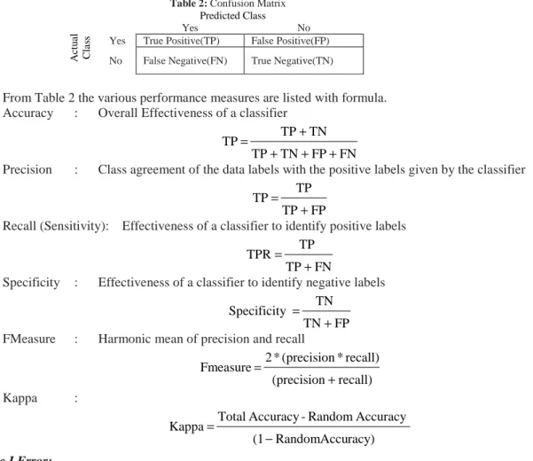
The confusion matrix is tabulated for every classifier with actual and predicted class which is denoted for binary classification. Either supervised or unsupervised the table generalizes the True Positive (TP), False Positive (FP), False Negative (FN) and True Negative (TN) for various calculation of performance for the classifiers.
Table 2: Confusion Matrix Predicted Class A ct u al C la ss
Yes No
Yes True Positive(TP) False Positive(FP)
No False Negative(FN) True Negative(TN)
From Table 2 the various performance measures are listed with formula. Accuracy : Overall Effectiveness of a classifier
FN FP TN TP TN TP TP + + + + =
Precision : Class agreement of the data labels with the positive labels given by the classifier
FP TP TP TP + =
Recall (Sensitivity): Effectiveness of a classifier to identify positive labels
FN TP TP TPR + =
Specificity : Effectiveness of a classifier to identify negative labels
FP TN TN y Specificit + =
FMeasure : Harmonic mean of precision and recall
recall) (precision recall) * (precision * 2 Fmeasure + =
Kappa :
racy) RandomAccu (1 Accuracy Random -Accuracy Total Kappa − =
Type I Error:
Inappropriate Elimination of true null hypothesis i.e., False Positive Error is Type I Error. Type I error is finding an effect that is present.
Type II Error:
The failure to reject a false null hypothes is False Negative Error and it is called Type II Error. Failing to detect an effect that is present.Using Weka software the Parkinsons dataset is preprocessed and the following Table 3
Table 3: Confusion Matrix for various classifiers
Algorithm Confusion Matrix
Bayes Net
C0 C1 Sum
C0 99 48 147
C1 6 42 48
NaiveBayes
C0 C1 Sum
C0 102 45 147
C1 6 42 48
ZeroR
C0 C1 Sum
C0 147 0 147
C1 48 0 48
OneR
C0 C1 Sum
C0 121 26 147
C1 17 31 48
WEO
C0 C1 Sum
C0 130 17 147
C1 8 40 48
C0 – Indicates Parkinson Disease C1- Healthy without Parkinson
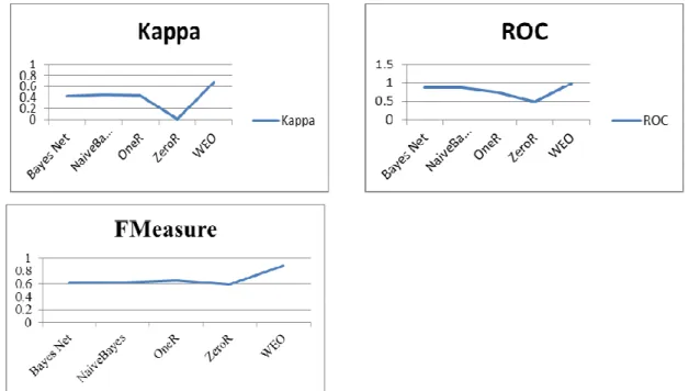
Table 4: Comparative Study of various classifiers with their performance measures
Performance Measure BayesNet NaiveBayes OneR ZeroR WEO
Accuracy (%) 72.30 73.84 77.94 75.38 87.17
Sensitivity 0.87 0.87 0.75 0.64 0.88
Specificity 0.67 0.69 1.00 0.82 0.76
Precision 0.46 0.48 0.56 0.54 0.87
Kappa 0.42 0.44 0.44 0.00 0.67
ROC 0.86 0.86 0.73 0.47 0.97
FMeasure 0.60 0.62 0.64 0.59 0.87
Fig. 1: Graph of various classifiers with their performance measures
Findings:
In addition to the above performance measures, the proposed research work analyses the penalty cost and its objective is to optimize the penalty cost in the case of imbalanced dataset. The penalty cost associated with labeling a person with Parkinson disease (C0) as negative (False Negative) is higher than and labeling a person without Parkinson disease (C1) as positive (False Positive). The goal of this article is to choose a classifier that result in minimal total penalty cost.
Total Cost = C (Fn) *FN + C (F) *FP+C (TP) + C (TN) …. (1)
From equ (1) usually the cost of classifying instances correctly will be considered as zero and the C (FN) > C (FP) i.e., the cost of False Negative will be greater than that of cost of False Positive.
Table 4: The Cost Penalty Confusion Matrix
Predicted Class
A
ct
u
al
C
la
ss
Yes No
Yes C(TP) C(FP)
No C(FN) C(TN)
The Table 4 designs the structure of Cost Penalty Confusion Matrix and it is usual practice to give a higher weightage for cost associated with False Negative than for false positive. Let us consider the cost of misclassifying an instance as FN is doubled (2*X) when compared to classifying the same instance as FP (X). For instance x is assumed as Rs. 1000, then the total penalty cost associated with classifiers are calculated by substituting in equ (1) are as follows:
Table 5: Penalty for various classifiers Classifiers Penal Cost for FN
(Rs.)
Penal Cost for FP (Rs.)
Total Penalty Cost (Rs.)
BayesNet 12000 48000 60000
NaiveBayes 12000 45000 57000
ZeroR 48000 0 48000
OneR 34000 26000 60000
WEO 16000 17000 23000
Conclusion:
The proposed model exhibited utmost accuracy of 87.17% with a robust kappa statistics measurement and roc degree indicated the strong stability of the model when compared to other classifiers. In medical dataset for classification problem type II error is significant than type I error. Penalty cost for misclassifying an instance with respect to type I error is Rs. X and with respect to type II is Rs.(2*X) . The objective of the proposed work is to minimize False Negative than False Positive. Thus the model proposed had lesser penalty cost considered with other classifier models. In addition to accuracy the proposed method also considers measures like sensitivity, specificity, precision, kappa, roc and Fmeasure. Since, the dataset is imbalanced where the class C0 represents the person with Parkinson disease and the class C1 represents the person who are healthy as(147,48) the scope of the future work is to remove noise and to handle the imbalanced dataset to use ensemble classifiers to improve the performance measures. Among the algorithms Weighted Empirical Optimization algorithm performance is much better than other algorithms on accuracy, sensitivity, specificity, precision, kappa, roc and Fmeasure. On the contrary Bayesnet and NaiveBayes produces lesser percentage of misclassified instances than the other algorithms of which False Negative is lesser than False Positive and the model proposed in this work results in a lesser penalty cost than other classifiers which is important for clinical data. In this article the data is imbalanced which has to be balanced to carry out feature selection in future work and also to compare with more classifiers to exhibit the concert of the proposed model.
REFERENCES
1. Ahlrichs, C., M. Lawo, 2013. Parkinson’s Disease Motor Symptoms in Machine Learning: A Review, http://arxiv.org/abs/1312.3825.
2. Genain, N., M. Huberth, R. Vidyashankar, 2014. Predicting Parkinson ’ S Disease Severity from Patient Voice Features. http://roshanvid.com/stuff/parkinsons.pdf.
3. Mathers, C., D.M. Fat, J.T. Boerma, W.H. Organization, 2008. The Global Burden of Disease : 2004 Update. Geneva, Switzerland: World Health Organization.
4. Chen, L., 2013. Computer-Aided Detection of Parkinson’s Disease Using Transcranial Sonography. In: Dissertation for Fulfillment of Requirements for the Doctoral Degree of the University of Lübeck from the Departments Information Technology. Vol Germany: University of Lübeck, 128. http://www.students.informatik.uni-luebeck.de/zhb/ediss1324.pdf.
5. Sateesh Babu, G., S. Suresh, 2013. Parkinson’s disease prediction using gene expression – A projection based learning meta-cognitive neural classifier approach. Expert Syst Appl., 40(5): 1519-1529. doi:10.1016/j.eswa.2012.08.070.
6. Bind, S., A.K. Tiwari, A.K. Sahani, 2015. A Survey of Machine Learning Based Approaches for Parkinson Disease Prediction. International Journal Computer Science Information Technology, 6(2): 1648-1655. http://www.ijcsit.com/docs/Volume 6/vol6issue02/ijcsit20150602163.pdf.
7. Holkar, P., P. Gatti, S. Meher, P. Sable, 2015. A Review on Parkinson Disease Classifier Using Patient Voice Features. International Journal Advance Research Electrical Electronics Instrumentation Engineering. 4(5): 3827-3830. http://www.ijareeie.com/upload/2015/may/5_A_review.pdf.
8. Rustempasic, I., M. Can, 2013. Diagnosis of Parkinson ’ s Disease using Principal Component Analysis and Boosting Committee Machines. SouthEast European Journal of Soft Computation., 2(1): 102-109. http://www.ius.edu.ba/sites/default/files/articles/51-145-1-PB.pdf.
9. Khemphila, A., V. Boonjing, 2012. Parkinsons Disease Classification using Neural Network and Feature selection. International School of Science Research Innovation, 6(4): 15-18. http://waset.org/publications/8538/parkinsons-disease-classification-using-neural-network-and-feature-selection.
10. Sakar, B.E., O. Kursun, 2014. Telemonitoring of changes of unified Parkinson ’ s disease rating scale using severity of voice symptoms. In: The 2nd International Conference on E-Health and Telemedicine. Vol Diagonastic Pathology, pp: 114-119.
11. Armañanzas, R., C. Bielza, K.R. Chaudhuri, P. Martinez-Martin, P. Larrañaga, 2013. Unveiling relevant non-motor Parkinson’s disease severity symptoms using a machine learning approach. Artificial Intelligence Medicine, 58(3): 195-202. doi:10.1016/j.artmed.2013.04.002.
12. Sriram, TV., M.V. Rao, G.V.S. Narayana, D. Kaladhar, T.P.R. Vital, 2013. Intelligent Parkinson Disease Prediction Using Machine Learning Algorithms. In: International Journal of Engineering and Innovative Technology (IJEIT). 3.
13. Khan, S.U., 2015. Classification of Parkinson’s Disease Using Data Mining Techniques. J Park Dis Alzheimer’s Dis., 2(1): 1-4.
Research Computation Science Software Engineering, 2(3): 298-304. http://www.ijarcsse.com/docs/papers/March2012/volume_2_Issue_3/V2I300135.pdf.
15. Rustempasic, I., M. Can, 2013. Diagnosis of Parkinson’s Disease using Fuzzy C - Means Clustering and Pattern Recognition. International University Sarajev, Fac Eng Nat Sci.
16. Kaladhar, D.S.V.G.K., Rao, P. Nageswara, 2010. Rajana Blvrn. Confusion Matrix Analysis For Evaluation Of Speech On Parkinson Disease Using Weka And Matlab. International Journal of Engineering Science Technology, 2(7): 2734-2737.
17. Jiawei Han, Micheline Kamber, Jian Pei , Data Mining Book, Southeast Asia Edition.
18. Suganya, P. and C.P. Sumathi, 2015. A Novel Metaheuristic Data Mining Algorithm for the Detection and Classification of Parkinson Disease, Indian journal of Science & Technology, 8: 14.
19. Suganya, P., C.P. Sumathi, Classifier rules in data mining – A Survey, IEEExplore.
20. Chitra Nasa and Suman, 2012. Evaluation of different classification technique for web data, International journal of computer Applications (0975-887), 52: 9.
21. Thair Nu Phyu, 2009. Proceedings of International Multi conference of Engineers and computer scientist I, IMECS, March 18 – 20, Survey of Classification Techniques in Data mining.
22. Divya Tomar and Sonali Agarwal, 2014. International Theory of Database Theory and Automation, 7(4): 99-128, A Survey on Pre-processing and Post-processing Techniques in Data Mining.
23. YogendraKumar Jain and Santhosh Kumar Bhandare, 2011. International Journal of Computer & Communication Technology, 2(VIII). Min Max Normalization Based Data Perturbation Method for Privacy Protection.
24. Mike, A Nalls and Cory Y. MCLean, 2015. The Lancet Neurology, 14(10): 1002-1009, Diagnosis of Parkinson’s disease on the basis of clinical and genetic classification: a population based modeling study. 25. Roberto Erro and Gabriella Santangelo, Journal of Parkinsonism and Restless legs syndrome, 5, Nonmotor