Classical and quantum scattering in optical systems

(1)

Classical and quantum scattering

in optical systems

PROEFSCHIRFT

ter verkrijging van

de graad van Doctor aan de Universiteit Leiden, op gezag van Rector Magniﬁcus Prof. Mr. P. F. van der Heijden,

volgens besluit van het College voor Promoties te verdedigen op woensdag 16 mei 2007

klokke 16.15 uur

door

Graciana Puentes

(2)

Promotor: Prof. dr. J. P. Woerdman Referent: Prof. dr. G. Nienhuis

Leden: Prof. dr. A. Lagendijk (Universiteit van Amsterdam / AMOLF) Dr. R. J. C. Spreeuw (Universiteit van Amsterdam)

Prof. dr. G. ’t Hooft Dr. M. P. van Exter

Prof. dr. C. W. J. Beenakker Prof. dr. J. M. van Ruitenbeek

The work reported in this Thesis is part of a research programme of ‘Stichting voor Funda-menteel Onderzoek der Materie’ (FOM) and was supported by the EU programme ATESIT. The image on the cover shows the exit basin diagram associated with light rays scattered by an optical cavity with a stochastic ray-splitting mechanism. The fractal nature of the basins is a typical feature of chaotic scattering. This is explained in detail in Chapter 3 (this Thesis). Casimir PhD Series, Delft-Leiden, 2007-02

(3)

CHAPTER

1

Introduction

1.1 Classical scattering in optical systems

Light scattering is a very broad topic which has a scientific history of over a century [1]. Generally speaking, light is scattered whenever it propagates in a material medium, because of its interaction with the molecules constituting the medium, which act as scattering centers. As a consequence, most of the light that we observe in daily life is scattered light. However, the arrangement of these molecules strongly determines the effectiveness of the scattering for a given input wave. For instance, in a perfect crystal the molecular scattering centra are so orderly arranged that the scattered output waves interfere destructively in such a way that only the propagation velocity of the incident wave is changed. Conversely, in a gas or a fluid, the statistical fluctuations of the molecular arrangement can cause significant scatter-ing. Depending on the nature of the interaction processes, light can be scattered elastically or inelastically [2]. In elastic (Rayleigh) scattering, the frequency of the scattered light is equiv-alent to that of the incident light. On the other hand, inelastic (Raman) scattering results in scattered light of different frequency than the incident. In this Thesis we will concentrate on elastic scattering processes where the frequency of the incident light is conserved. Addition-ally, we will restrict our analysis to linear scattering processes, where this linearity refers to the amplitude of the light field. A scattering process can be consider linear when, for a sum of incident input waves, the scattered output wave is a linear superposition of the incident ones. Such linear processes can be described by a scattering matrix, which maps input and output waves. In this context, we take a broad definition of an elastic light scattering process; namely, any optical process that changes the direction of the wave-vector of the light. Thus a scattering process can range from Rayleigh scattering by a point particle to refraction by a lens.

(8)

equa-tions. The interaction of such a field with the molecules in a material medium can modify its spatial distribution, frequency or polarization. The exact way in which these degrees of freedom are modified depend on the specific properties of the scattering medium, which can be described at different length scales. For example in Ref. [3], three levels of description are identified based upon three length scales. These levels are classified as macroscopic: on scales much larger than the mean free pathl, mesoscopic: on scales of the order of the mean free pathl and microscopic: on scales comparable to the wavelength of the lightλ. How-ever, in this Thesis we are exclusively interested in the changes produced by the scattering process on the electromagnetic field, thus regarding the scattering medium as a black box. Within such approach, the medium can be described by a phenomenological set of parame-ters, usually arranged to form a matrix. The size and properties of such matrix depend on the particular degrees of freedom of the field one is interested in. For example, when dealing with polarization degrees of freedom, the scattering process can be represented by a 4×4 real-valued matrix, the so called Mueller matrix [4]. On the other hand, when dealing with propagation of rays of light through an astigmatic paraxial optical device, the information about the medium is contained in a 2×2 real-valued symplectic matrix, the so calledABCD

matrix [5]. In the following subsections we give explicit expressions for the Mueller matrix and theABCDmatrix of a generic optical system, which are used in the context of polariza-tion scattering and ray scattering, respectively.

1.1.1 Polarization scattering

The basic elements of a classical light scattering experiment are an incident field which il-luminates a scattering medium and a detector which measures the intensity of the scattered field (see Fig. 1.1). For a single spatial mode of the incident field (kin), here represented by

a plane-wave propagating in a given direction ˆkin, the effect of a single scattering event is

to change the direction of propagation of the ﬁeld, so that the scattered ﬁeld is in the output plane-wave mode (kout) characterized by the direction ˆkout. Here|kin|=|kout|, since we are

considering elastic scattering processes. The electric ﬁeld, which determines the polarization,

Scattered field

Detector

k

r

k

r

E

_E

(9)

1.1 Classical scattering in optical systems

is here represented by the complex vectorE∈C2_:_E₌_E

1ˆ1+E2ˆ2, on a plane orthogonal to

the direction of propagation ˆk. Note that the three real-valued unit vectors {ˆ1,ˆ2,kˆ}define an orthogonal Cartesian frame. Since the polarizationEis a transverse degree of freedom, a transformation on the spatial properties of the light beam (by scattering) is always ac-companied by an intrinsic transformation on the polarization of the light beam. Any linear transformation of the polarization properties of the beam by scattering can be represented in the Mueller-Stokes formalism. Within this formalism, the electric field is fully specified by the real-valued 4-dimensional Stokes vectorS∈R2:S= (S0,S1,S2,S3); namely:

S0 ≡ |E1|2+|E2|2∝I

S1 ≡ |E2|2− |E1|2∝I0◦−I90◦

S2 ≡ E1E2∗+E2E1∗∝I45◦−I−45◦

S3 ≡ i(E1E2∗−E2E1∗)∝IRHC−ILHC.

(1.1) If we identify the directions ˆ1 and ˆ2 with vertical (90◦) and horizontal (0◦) polarizations respectively, thenS0is proportional to the total intensity of the beam,S1is proportional to the

difference in intensities between horizontal and vertical linearly polarized components,S2is

proportional to the difference in intensities between linearly polarized components oriented at 45◦and−45◦andS3 is proportional to the difference in intensities between right hand

RHCand left handLHCcircularly polarized components. It should be stressed that the real valued 4-dimensional Stokes vector contains the same information as the complex valued 2× 2 coherency matrixJ[6]. The advantage of the Mueller-Stokes formalism is that it is directly related with measurable quantities, i.e., intensities. The only restriction for a Stokes vector to represent a physical polarization state is that∑i(Si)2≤(S0)2(i=1,2,3). Additionally,

any optical system, which transforms an input Stokes vectorSininto an output Stokes vector

Sout, can be characterized by a 4×4 Mueller matrix (M), whose 16 real elements map the

polarization state of the input and output beams by:

Sout=MSin. (1.2)

In this Thesis we considered only passive or non-amplifying optical media such that the output intensity is not larger than the input intensity, in other words for all our scattering mediaS0,out≤S0,in. However, it should be noted that an active medium, i.e., a medium with

gain, can in principle also be represented by a Mueller matrix. This is because classically, a medium with gain, is formally equivalent to a medium with absorption, up to a sign, and scattering media with polarization dependent absorption, i.e., dichroic scattering media, are fully described in the Mueller-Stokes formalism.

(10)

properties of the outgoing beam are measured with a mode-insensitive device, the scattered ﬁeld might appear partially depolarized. The degree of polarization (PF) of a light beam is

deﬁned by

PF=

(S1)2+ (S2)2+ (S3)2

S0 ,

(1.3) where 0≤PF≤1. Fully polarized light hasPF=1 while unpolarized light hasPF=0, the

intermediate values forPF correspond to partially polarized light. The main mechanism of

depolarization that we analyze in this Thesis is given by the coupling of polarization and spatial degrees of freedom. A typical example of this is the case of a beam of light initially prepared in a single plane-wave mode (kin) that is incident on an inhomogeneous medium.

Due to the spatial inhomogeneities in the medium, the beam suffers multiple scattering and, as a result, it emerges as a (partially) incoherent superposition of many plane-waves (kout). Even

when each of the output modes is fully polarized, the output beam appears to be (partially) depolarized when its spatial information is averaged out in a multi-mode detection set-up.

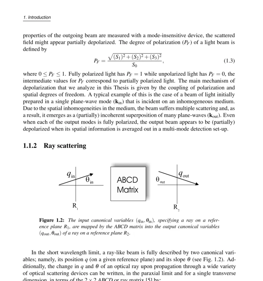
1.1.2 Ray scattering

ABCD

Matrix

in

q

out

R

_R

Figure 1.2: The input canonical variables (qin,θin), specifying a ray on a refer-ence plane R1, are mapped by the ABCD matrix into the output canonical variables

(qout,θout)of a ray on a reference plane R2.

In the short wavelength limit, a ray-like beam is fully described by two canonical vari-ables; namely, its positionq(on a given reference plane) and its slopeθ(see Fig. 1.2). Ad-ditionally, the change inqandθ of an optical ray upon propagation through a wide variety of optical scattering devices can be written, in the paraxial limit and for a single transverse dimension, in terms of the 2×2ABCDor ray matrix [5] by:

qout θout = A B C D qin θin . (1.4)

(11)

1.2 Quantum scattering in optical systems

round trip of a ray inside such a cavity can be represented, in the paraxial approximation, by anABCDmatrix and can thus be interpreted as a linear optical ray scattering process.

1.2 Quantum scattering in optical systems

The quantum aspects of scattering in optical systems that are highlighted in our work refer to the quantum nature of the light that is incident on different scattering media. At the single-photon level, the quantum nature of light is revealed by the quantum field fluctuations, which can be seen as a consequence of the Heisenberg uncertainty relations between the electric and magnetic fields [7]. In this regard, the effect of multiple scattering on single-photon spatial correlations has been recently investigated in Ref. [8]. For photon pairs the quantum nature of light can also manifest itself by the mutual entanglement between the two photons belonging to the pair; this topic is addressed in this Thesis.

1.2.1 Entangled photons

A pair of photons is considered ‘entangled’ when a measurement on one of the two photons belonging to the pair completely determines the outcome of measurements on the other one, regardless of the distance between the photons. These non-local correlations, referred to as quantum entanglement, can not be explained in terms of any local classical theory and have puzzled many physicist starting by Einstein, Podolosky and Rosen [9], in 1935. In our scattering experiments with quantum light, we have concentrated on entangled photon pairs, where the incident state of light is entangled in the polarization degrees of freedom. A typical example is the polarization-singlet Bell state:

|ψ−₌|H1V2 − |_√ V1H2

2 , (1.5)

where 1 and 2 label the two photons belonging to the pair, and(H,V)label horizontal and vertical polarizations, respectively. In fact, this state contains maximal information about the correlations of the two photons but minimal information about the polarization state of each individual photon. Thus if we measure the polarization of photon 1, and we ﬁnd that it is verticalV, then we automatically know that the outcome of a similar measurement on photon 2 would yieldH. Note that the anti-correlation between the polarization state of each photon belonging to the singlet is valid inanypolarization basis.

1.2.2 Light scattering with entangled photons

(12)

as the photons are detected in a single spatial mode [13, 14]. Therefore, it appears to be rele-vant to characterize entanglement decay upon linear scattering processes in combination with multi-mode detection, and that is indeed the central topic of this Thesis.

The main concept behind light scattering with polarization entangled photons is that a scattering process can couple polarization and spatial degrees of freedom of light. The details of this coupling depend on the speciﬁc scattering medium. If the scattered photons are then detected in a momentum insensitive way (multi-mode detection), all the spatial information of the scattering process encoded in the photons is averaged or traced over, leaving each photon in a mixed polarization state. As one might expect, this transition from pure to mixed state reduces the degree of entanglement; this has been theoretically explored in recent papers [13, 14].

The output polarization state of the scattered photons can be calculated once we know the phenomenological polarization matrix (i.e., the Mueller matrixM) characterizing the scatter-ing medium. For an input state given by a pair of photons, initially prepared in the polarization singlet state

ρin=|ψ−ψ−|, (1.6)

and for a local scattering medium, i.e., a medium acting on a single photon of the entangled pair, the scattered photon-pair, which is in the mixed polarization stateρout, can be written in

areshufﬂedbasis, here denoted by the superscript (R), as [15]: ρR

out=MρinR, (1.7)

where the matrixM maps the input and output polarization states of the photon pairs.M is linearly related to the classical Mueller matrixMof the scattering medium, this is explained in detail in Chapter 8.

Eq.(1.7) suggests that the study of a local scattering process acting on a pair of photons is an alternative (and rather sophisticated) way of studying a depolarizing process. In other words, it is a non-standard way of measuring the Mueller matrixM(orM) of a depolarizing medium. We stress that the fact that a scattering experiment with two-photon light reveals the same amount of information on the scattering medium as a similar experiment with a classical beam of light is only true as long as we analyze, as we do in this Thesis,localscattering media. That is, scattering media located on the path of a single photon of the entangled pair. Nevertheless, although we only experimented with local media, our mathematical formalism still applies to bi-local scattering media, which can be written as the (outer) product of two Mueller matrices acting on each photon of the pair, and to non-local scattering media, which can be written as an inseparable (two-photon) Mueller matrix [15].

Finally, it is important to stress that one of the main goals in our scattering experiments with entangled photons was to engineer (mixed) quantum states of light in a controllable way (see Chapter 7 and Chapter 8). As a consequence, in most of our experiments with quantum light, our target is the two-photon scattered stateρoutrather than the classical Mueller matrixM.

(13)

1.3 Thesis overview

In this Thesis we analyzed the effect of a large variety of linear scattering processes both on classical light (Chapter 4-5) and on two-photon quantum light (Chapter 6-9). The main part of this analysis refers to the polarization degrees of freedom of scattered light where the medium parameters are phenomenologically described within the Mueller matrix formal-ism. The main tool used for this characterization is multi-spatial-mode optical polarization tomography, both in its classical and quantum versions.

Additionally, in fact as a starter for this Thesis, we have numerically investigated dynam-ical properties of ray scattering in optdynam-ical cavities by using Hamiltonian optics (Chapter 2-3). The paraxial description of light rays in such optical cavities is described within theABCD

matrix formalism.

We describe the contents of the Chapters in more detail below:

• In Chapter 2 we report a numerical investigation of theparaxialray dynamics of light scattered by an optical cavity with a stochastic ray-splitting mechanism. We show the results obtained for the paraxial map of the system, applying standard tools from non-linear dynamics. A discussion on the mixing properties of the system and their relation with the Kolmogorov-Sinai (KS) entropy is included.

• In Chapter 3 we presents theexactray dynamics in an optical cavity with a ray splitting mechanism, similar to the one introduced in Chapter 2. By using exact Hamiltonian optics, we show that such a simple scattering device presents a surprisingly rich chaotic ray dynamics.

• In Chapter 4 we describe the theoretical background related to our experiments on classical light depolarization due to multi-mode scattering. The key theoretical concept we introduce is the effective Mueller matrix, which describes our spatial multi-mode detection set-up.

• In Chapter 5 we show experimental results on classical light depolarization due to multi-mode scattering. By means of polarization tomography, we characterize the de-polarizing power and the polarization entropy of a broad class of optically scattering media.

• In Chapter 6 we report experimental results on a controllable source of spatial deco-herence for polarization entangled photons, based upon commercially available wedge depolarizers. A full characterization of the scattered states, by means of quantum to-mography, shows that such a scattering device can be used for synthesizing Werner-like states on demand.

• In Chapter 7 we present experimental results on the effect of different scattering process on polarization entangled photons. The scattering media are grouped in isotropic, bire-fringent and dichroic scattering. We compare the experimental results with a phenom-enological model based upon the description of a scattering process as a quantum map.

(14)

can be used for entangled-mixed state engineering. We report an experimental scheme suitable for maximally entangled mixed states engineering and the corresponding ex-perimental results.

(15)

CHAPTER

2

Paraxial ray dynamics in an optical cavity with a

beam-splitter.

In this Chapter1we present a numerical investigation of the ray dynamics in an optical cavity when a ray splitting mechanism is present; we focus mainly on the paraxial limit. The cavity is a conventional two-mirror stable resonator and the ray splitting is achieved by inserting an optical beam splitter perpendicular to the cavity axis. We show the results obtained for the paraxial map of the system [16], applying standard tools from non-linear dynamics, such as Poincar´e Surface of Section (SOS), exit basin diagrams, escape rate and Lyapunov exponents. Furthermore, a discussion about the mixing properties of the system and their relation with the Kolmogorov-Sinai (KS) entropy is included. In the paraxial limit the ray dynamics is irregular and both the Lyapunov exponent and the KS entropy are positive; however, chaos does not occur.

(16)

2.1 Introduction

A beam splitter (BS) is an ubiquitous optical device in wave optics experiments, used e.g., for optical interference, homodyning, etc. In the context of geometrical optics, the action of a BS is to split a light ray into a transmitted or a reﬂected ray. Ray splitting provides a useful mechanism to generate chaotic dynamics in pseudointegrable [17] and soft-chaotic [18–21] closed systems. In this Chapter we exploit the ray splitting properties of a BS in order to build an open paraxial cavity which shows irregular ray dynamics as opposed to the regular dynamics displayed by a paraxial cavity when the BS is absent.

D

M

L

R

BS

Figure 2.1:Schematic diagram of the cavity model. Two subcavities of length L1and L2are coupled by a BS. The total cavity is globally stable for L=L1+L2<2R.Δ= L1−L/2represents the displacement of the BS with respect to the center of the cavity.

Optical cavities can be classified asstableorunstabledepending on the focussing prop-erties of the elements that compose it [5]. An optical cavity formed by 2 concave mirrors of radiiRseparated by a distanceLis stable whenL<2Rand unstable otherwise. If a light ray is injected inside the cavity through one of the mirrors it will remain confined indefinitely inside the cavity when the configuration is stable but it will escape after a finite number of bounces when the cavity is unstable (this number depends on the degree of instability of the system). Both stable and unstable cavities have been extensively investigated since they form the basis of laser physics [5]. Our interest is in a composite cavity which has both aspects of stability and instability. The cavity is made by two identical concave mirrors of radiiR sepa-rated by a distanceL, whereL<2Rso that the cavity is globally stable. We then introduce a beam splitter (BS) inside the cavity, oriented perpendicular to the optical axis (Fig. 2.1). In this way the BS defines two subcavities. The main idea is that depending on the position of the BS the left (right) subcavity becomesunstablefor the reflected rays whenL1(L2) is

bigger thanR, whereas the cavity as a whole remains alwaysstable(L1+L2<2R) (Fig. 2.2).

(17)

2.1 Introduction

R

L

1

L

2

BS

L =L <R

1 2 ( a)

BS

R

L >R>L

1 2

( b)

BS

R

L >R>L

2 1

( c)

y

L

1

L

₂

L

2

L

1

Figure 2.2: The different positions of the beam splitter determine the nature of the subcavities. In (a) the BS is in the middle, so the 2 subcavities are stable, in (b) the left cavity is unstable and the right one is stable, and (c) the unstable (stable) cavity is on the right (left) (b).

Lyapunov exponents) and mixing (conﬁnement inside the system) form the skeleton of chaos [22].

(18)

BS

L

1

L

₂

q

Z

z=const

Figure 2.3: A ray on a reference plane (z=const) perpendicular to the optical axis (Z) is speciﬁed by two parameters: the height q above the optical axis and the angleθ between the direction of propagation and the same axis. When a ray hits the surface of the BS, which we choose to coincide with the reference plane, it can be either reﬂected or transmitted with equal probability (p). For a50/50beam splitter p=1/2.

Our system bears a close connection with the stability of a periodic guide of paraxial lenses as studied by Longhi [30]. While in his case acontinuousstochastic variableεn

repre-sents a perturbation of the periodic sequence along which rays are propagated, in our case we have adiscretestochastic parameter pnwhich represents the response of the BS to an

inci-dent ray. As will be shown in section 2.2, this stochastic parameter can take only two values, either +1 for transmitted rays or -1 for reﬂected rays; in this sense, our system (displayed as a paraxial lens guide in Fig. 2.4) allows a surprisingly simple realization of a bimodal stochastic dynamics.

2.2 Ray dynamics and the paraxial map

The time evolution of a laser beam inside a cavity can be approximated classically by using the ray optics limit, where the wave nature of light is neglected. Generally, in this limit the propagation of light in a uniform medium is described by rays which travel in straight lines, and which are either sharply reﬂected or refracted when they hit a medium with a different refractive index. To fully characterize the trajectory of a ray in a strip resonator or in a resonator with rotational symmetry around the optical axis, we choose a reference plane

z=constant(perpendicular to the optical axis ˆz), so that a ray is speciﬁed by two parameters: the heightqabove the optical axis and the angleθbetween the trajectory and the same axis. Therefore we can associate a ray of light with a two dimensional vectorr= (q,θ). This is illustrated in the two mirror cavity show in Fig. 2.3, where the reference plane has been chosen to coincide with the beam splitter (BS). Given such a reference planez, which is also called Poincar´e Surface of Section (SOS) [23], a round trip (evolution between two successive reference planes) of the ray inside the cavity can be calculated by the monodromy matrix

Mn, in other wordsrn+1=Mnrn, where the indexn determines the number of round trips.

(19)

2.2 Ray dynamics and the paraxial map

reference periodic orbit. A periodic orbit is said to bestableif|TrMn|<2. In this case nearby

rays oscillate back and forth around the stable periodic orbit with bounded displacements both inqandθ. On the other hand when|TrMn| ≥2 the orbit is said to be unstable and rays that

are initially near this reference orbit become more and more displaced from it.

For paraxial trajectories, where the angle of propagation relative to the axis is taken to be very small (i.e., sin(θ)∼=tan(θ)∼=θ), the reference periodic trajectory coincides with the optical axis and the monodromy matrix is identical to the ABCD matrix of the system. The ABCD matrix or paraxial map of an optical system is the simplest model one can use to describe the discrete time evolution of a ray in the optical system [5]. Perhaps the most interesting and important application of ray matrices comes in the analysis of periodic fo-cusing (PF) systems in which the same sequence of elements is periodically repeated many times down in cascade. An optical cavity provides a simple way of recreating a PF system, since we can think of a cavity as a periodic series of lenses (see Fig. 2.4). In the framework of geometric ray optics, PF systems are classiﬁed, as are optical cavities, as either stable or unstable.

Z Z Z

2L

Z

r

_r

Z

Figure 2.4:A ray bouncing inside an optical cavity can be represented by a sequence of lenses of focus f=2/R, followed by a free propagation over a distances Ln. Due to

the presence of the BS, the distance Lnvaries stochastically between L1or L2.

Without essential loss of generality we restrict ourselves to the case of a symmetric cavity (i.e., two identical spherical mirrors of radius of curvatureR). We take the SOS coincident with the surface of the BS. After intersecting a given reference planezi, a transmitted

(re-ﬂected) ray will undergo a free propagation over a distanceL2(L1), followed by a reﬂection

on the curved mirrorM2(M1), and continue propagating over the distanceL2(L1), to hit the

surface of the beam splitter again atzi+1. In Fig. 2.4 the sequence ofzirepresents the

succes-sive reference planes after a round trip. In the paraxial approximation each round trip (time evolution between two successive intersections of a ray with the beam splitter) is represented by:

qn+1= Anqn+Bnθn,

θn+1= Cqn+Dnθn, (2.1)

where

(20)

and

Ln=

L+pna

2 .

We have deﬁnedL=L1+L2 anda=L2−L1; the stochastic parameter pn is distributed

equally among−1 and+1 for our 50/50 BS, and determines whether the ray is transmitted (pn=1) or is reﬂected (pn=−1).

The elements of the ABCD matrix depend on the indexnbecause of the stochastic re-sponse of the BS, which determines the propagation for the ray in subcavities of different length (eitherL1or L2). In this way a random sequence of reﬂections (pn=1) and

trans-missions (pn=−1) represents a particular geometrical realization of a focusing system. If

we want to study the evolution of a set of rays injected in the cavity with different initial conditions(q0,θ0), we have two possibilities, either use thesamerandom sequence of

re-ﬂections and transmissions for all rays in the set or use adifferentrandom sequence for each ray. In the latter case, we are basically doing an ensemble average over different geometrical conﬁgurations of focusing systems. As we shall see later it is convenient, for computational reasons, to adopt the second method.

The paraxial map of Eq. (2.1) describes an unbounded system. That is, a system for which rays are allowed to go infinitely far from the cavity axis. In order to describe a physical parax-ial cavity we have to keep the phase space bounded, i.e., it is necessary to artificparax-ially introduce boundaries for the position and the angle of the ray [31]. The phase space boundaries that we have adopted to decide whether a ray has escaped after a number of bounces or not are the beam waist (w0) and the diffraction half-angle (Θ0) [5] of a gaussian beam confined in

a globally stable two-mirror cavity. Measured at the center of the cavity, the waist and the corresponding diffraction half-angle result in:

w20=

Lλlight

π

2R−L

4L (2.2)

Θ0=arctan(λlight πw0)

(2.3)

Where we refer to the optical wavelength asλlightin order to avoid confusion with the

Lya-punov exponentλ. For our cavity conﬁguration we assume R=0.15 m, L=0.2 m and

λlight=500 nm, from which follows thatw0=5.3×10−5 m andΘ0=0.15×10−3rad.

One should keep in mind that this choice is somewhat arbitrary and other choices are cer-tainly possible. The effect of this arbitrariness on our results will be discussed in detail in subsection 2.3.4.

(21)

2.3 Numerical results

2.3.1 Poincar´e surface of section (SOS)

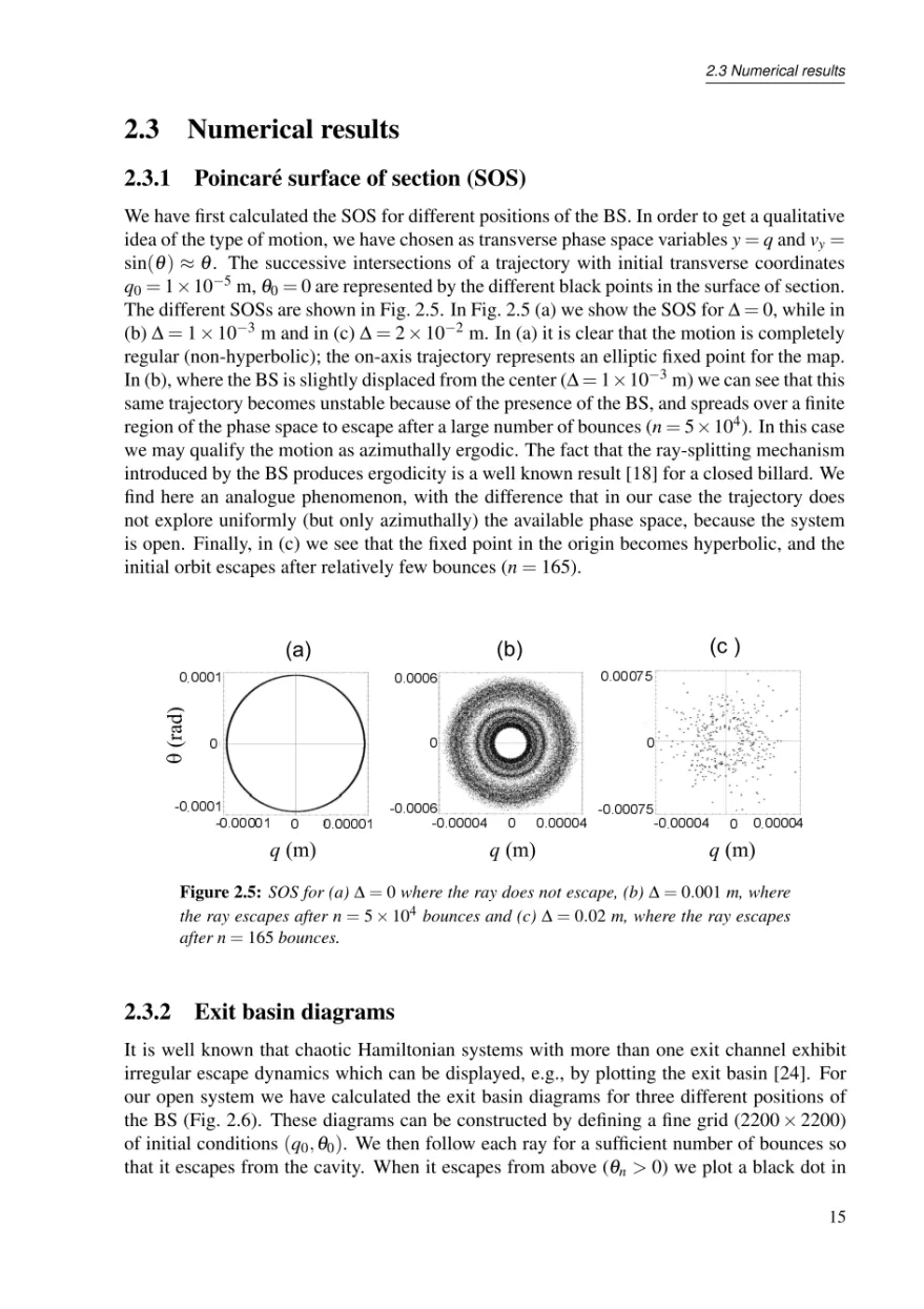
We have ﬁrst calculated the SOS for different positions of the BS. In order to get a qualitative idea of the type of motion, we have chosen as transverse phase space variablesy=qandvy=

sin(θ)≈θ. The successive intersections of a trajectory with initial transverse coordinates

q0=1×10−5m,θ0=0 are represented by the different black points in the surface of section.

The different SOSs are shown in Fig. 2.5. In Fig. 2.5 (a) we show the SOS forΔ=0, while in (b)Δ=1×10−3_{m and in (c)}_Δ₌₂_×₁₀−2_{m. In (a) it is clear that the motion is completely}

regular (non-hyperbolic); the on-axis trajectory represents an elliptic ﬁxed point for the map. In (b), where the BS is slightly displaced from the center (Δ=1×10−3_{m) we can see that this}

same trajectory becomes unstable because of the presence of the BS, and spreads over a finite region of the phase space to escape after a large number of bounces (n=5×104). In this case we may qualify the motion as azimuthally ergodic. The fact that the ray-splitting mechanism introduced by the BS produces ergodicity is a well known result [18] for a closed billard. We find here an analogue phenomenon, with the difference that in our case the trajectory does not explore uniformly (but only azimuthally) the available phase space, because the system is open. Finally, in (c) we see that the fixed point in the origin becomes hyperbolic, and the initial orbit escapes after relatively few bounces (n=165).

(a)

q

(rad)

-x

q

(m)

(b)

q

(m)

(c )

q

(m)

Figure 2.5:SOS for (a)Δ=0where the ray does not escape, (b)Δ=0.001m, where the ray escapes after n=5×104bounces and (c)Δ=0.02m, where the ray escapes after n=165bounces.

2.3.2 Exit basin diagrams

It is well known that chaotic Hamiltonian systems with more than one exit channel exhibit irregular escape dynamics which can be displayed, e.g., by plotting the exit basin [24]. For our open system we have calculated the exit basin diagrams for three different positions of the BS (Fig. 2.6). These diagrams can be constructed by defining a fine grid (2200×2200) of initial conditions(q0,θ0). We then follow each ray for a sufficient number of bounces so

(22)

the corresponding initial condition, whereas when it escapes from below (θn<0) we plot a

white dot.

In Fig. 2.6 (a) we show the exit basins forΔ=0.025 m, the uniformly black or white regions of the plot correspond to rays which display a regular dynamics before escaping, and the dusty region represents the portion of phase space where there is sensitivity to initial conditions. In Fig. 2.6 (b), we show the same plot forΔ=0.05 m, and in (c) forΔ=0.075 m.

The exit basin plots in Fig. 2.6 illustrate how the scattering becomes more irregular as the BS is displaced from the center. In particular, we see how regions of regular and irregular dynamics become more and more interwoven asΔincreases. As a reverse trend, for small values ofΔas in Fig. 2.6 (a), there is a single dusty region with a uniform distribution of white and black dots in which no islands of regularity are present.

0 -5.3x10-5

5.3x10-5 -0.0015

0 0.0015

0 -5.3x10-5

5.3x10-5 -5.3x10-5 0 5.3x10-5

q

0

Figure 2.6:Exit basins for (a)Δ=0.025 m, (b)Δ=0.05 m and (c)Δ=0.075 m.

2.3.3 Escape rate and Lyapunov exponent

The dynamical quantities that we have calculated next are the escape rateγand the Lyapunov exponentλ. The escape rate is a quantity that can be used to measure the degree of openness of a system [31]. For hard chaotic systems (hyperbolic), the numberNnof orbits still

con-tained in the phase space after a long time (measured in number of bouncesn) decreases as

N0exp(−γn)[32]. The Lyapunov exponent is the rate of exponential divergence of nearby

trajectories.

Since bothλ andγ are asymptotic quantities they should be calculated for very long times. In our system long living trajectories are rare. In order to pick them among the grid of initial conditions (N0) one has to increaseN0beyond our computational capability. To

overcome this difﬁculty we choose a different random sequence for each initial condition. In this way we greatly increase the probability of picking long living orbits given by particularly stable random sequences. These long living orbits in turn make possible the calculation of asymptotic quantities such asλ orγ.

The escape rateγwas determined by measuringNn, as the slope of a lg(Nn/N0)versusn

(23)

2.3 Numerical results

We have calculated the dependence ofγon the displacement of the BS (Δ) from the center of the cavity, where 0≤Δ≤L/2. Since forΔ>R−L/2 the left subcavity becomes unstable, it would seem natural to expect that this position of the BS would correspond to a critical point. However, we have found by explicit calculation of both the Lyapunov exponent and the escape rate, that such a critical point does not manifest itself in a sharp way, rather we have observed a ﬁnite transition region (as opposed to a single point) in which the functional dependence ofλ andγ changes in a smooth way. In Fig. 2.7 (a) we show the typical be-havior of Nn/N0vsn in semi-logarithmic plot for three different positions of the BS. The

displacements of the BS areΔ=0.0875 m, 0.05 m and 0.03125 m, and the corresponding slopes (escape rateγ measured in units of the inverse number of bouncesn) of the linear ﬁt areγ =0.17693 n−1_{, 0.05371}_n−1 _{and 0.01206} _n−1_{respectively. We have found that the}

decay is exponential only up to a certain time (approximately 70−1000 bounces depending on the geometry of the cavity) due the discrete nature of the grid of initial conditions.

In Fig. 2.7 (b) we see thatγ increases withΔ, revealing that for more unstable conﬁg-urations there is a higher escape rate, as expected. It is also interesting to notice that the exponential decay ﬁts better when the beam splitter is further from the center position, since this leads to smaller stability of the periodic orbits of the system. However, the dependence of the escape rate with the position of the BS is smooth and reveals that the only critical displacement, where the escape rate becomes positive, isΔ=0.

As a next step, we have calculated the Lyapunov exponentλ for the paraxial map;λ is a quantity that measures the degree of stability of the reference periodic orbit. For a two-dimensional hamiltonian map there are two Lyapunov exponents (λ1, λ2) such that λ1+

λ2=0. In the rest of the Chapter we shall indicate withλ the positive Lyapunov exponent

which quantiﬁes the exponential sensitivity to the initial conditions. We have calculatedλ for the periodic orbit on axis, using the standard techniques [33], and we have found that the Lyapunov exponent grows from zero with the distance of the BS from the center (Fig. 2.7 (c)). Therefore, the only critical point revealed by the ray dynamics is again the center of the cavity (Δ=0), where the magnitudes change from zero to a positive value.

The fact that the Lyapunov exponent of our paraxial systemdoesbecome positive (forΔ= 0) is rather surprising on its own right. Apparently, the presence of the BS with its stochastic nature introduces exponential sensitivity to initial conditions in the system for everyΔ=0, even when both subcavities are stable. This surprise can be explained by taking into account the probabilistic theorem by Furstenberg on the asymptotic limit of the rate of growth of a random product of matrices (RPM) [34]. From this theorem we expect that the asymptotic behavior of the product of a uniform random sequenceMnofD×Dmatrices, and for any

nonzero vectory∈ℜD:

lim

n→∞ 1

nln|Mny|Ω=λ1>0, (2.4)

whereλ1is the maximum Lyapunov exponent of the system, and the angular brackets indicate

the average over the ensembleΩof all possible sequences. This means that for RPM the Lyapunov exponent is a non-random positive quantity. In general, it can be said that there is a subspace Ω∗ of random sequences which has a full measure (probability 1) over the whole space of sequencesΩfor which nearby trajectories deviate exponentially at a rateλ1.

(24)

D(m) Ly apunov E xponent (n -1 ) E scape ra te (n -1 ) D(m) l -g (n -1 ) D l g l g ln (N t/N o) Time (n)

( c )

( b )

( d )

( a )

Figure 2.7:(a) Linear ﬁts used to calculate the escape rate for three different geomet-rical conﬁgurations of the cavity given byΔ=0.03125m,Δ=0.05m andΔ=0.0875

m. The time is measured in number of bounces(n). The slopeγis in units of the inverse of time(n−1). Fig. (b) shows the escape rateγ(n−1)as a function ofΔ. Fig. (c) corre-sponds to different Lyapunov exponentsλ(n−1₎_{as the BS moves from the center}_Δ₌₀ to the leftmost side of the cavityΔ=0.10m. Fig. (d) shows the difference betweenλ−γ

(n−1₎_{, which is a positive bounded function.}

limit, they do not change the logarithmic average (Eq. 2.4) [35]. We have veriﬁed this result, calculating the value ofλ for different random sequencesωi, in the asymptotic limit n=

100000 bounces, and we obtained in all cases the same Lyapunov exponent.

2.3.4 Mixing properties

Dynamical randomness is characterized by a positive Kolmogorov-Sinai (KS) entropy per unit time hKS[36]. In closed systems, it is known that dynamical randomness is a direct

consequence of the exponential sensitivity to initial conditions given by a positive Lyapunov exponent. On the other hand, in open dynamical systems with a single Lyapunov exponentλ, the exponential sensitivity to initial conditions can be related tohKSthrough the escape rate

γ, by the relation [27]:

λ=h_KS+γ. (2.5)

(25)

neighbor-2.4 Summary

hood of the unstable reference periodic orbit at an exponential rateγ, and the other one is a dynamical randomness because of transient chaotic motion near this unstable orbit [27]. This dynamical randomness is a measure of the degree of mixing of the system and as mentioned before is quantiﬁed byhKS. Therefore, for a givenλ, the larger the mixing is, the smaller the

escape rate, and viceversa. From Figs. 2.7 (b,c) it is evident that the Lyapunov exponent and the escape rate have the same smooth dependence on the BS displacementΔand thatγ≤λ. We have calculated the differenceλ−γ>0 for our system and the result is shown in Fig. 2.7 (d).

The actual value ofγ(Δ)depends, for a ﬁxed value ofΔ, on the size of the phase space accessible to the system [31], that is, it depends on w0andθ0. We veriﬁed this behavior

by successively decreasingw0andθ0by factors of 10 (see Table 2.1), and calculatingγfor

each of these phase space boundaries. It is clear from these results thatγ increases when the size of phase space decreases; in fact for w0,θ0≈0, one should get λ →γ and the

cavity mixing property should disappear. It should be noted that the increase ofγ when decreasing the size of the accessible phase space(ω0,θ0)is a general tendency, independent

of the chosen boundaries. It is important to stress that, although the randomness introduced (w0,θ0) ×100 ×10−1 ×10−2 ×10−3

γ 0.17639 0.17596 0.19559 0.25259

Table 2.1:Escape rate for different phase space boundaries. As the boundary shrinks

γ(Δ)tends to the corresponding value ofλ(Δ) =0.29178n−1_{. In these calculations the} displacement of the BS wasΔ=0.0875m.

by the stochastic BS is obviously independent from the cavity characteristics,λ andγ show a clear dependence on the BS position. When the BS is located at the center of the cavity it is evident for geometrical reasons that the ray splitting mechanism becomes ineffective:

λ=0=γ. These results conﬁrm what we have already shown in the SOS (Fig. 2.5).

2.4 Summary

(26)

(27)

CHAPTER

3

Chaotic ray dynamics in an optical cavity with a beam-splitter

In this Chapter we investigate the exact ray dynamics in an optical cavity when a ray splitting mechanism is present1_{. The cavity is a conventional two-mirror stable resonator} and the ray splitting is achieved by inserting an optical beam splitter perpendicular to the cavity axis. Using exact Hamiltonian optics, we show that such a simple device presents a surprisingly rich chaotic ray dynamics.

(28)

3.1 Introduction

In this Chapter we present a very simple optical cavity whose ray dynamics is nevertheless fully chaotic. Our starting point is the fact that a two-mirror optical cavity can bestableor

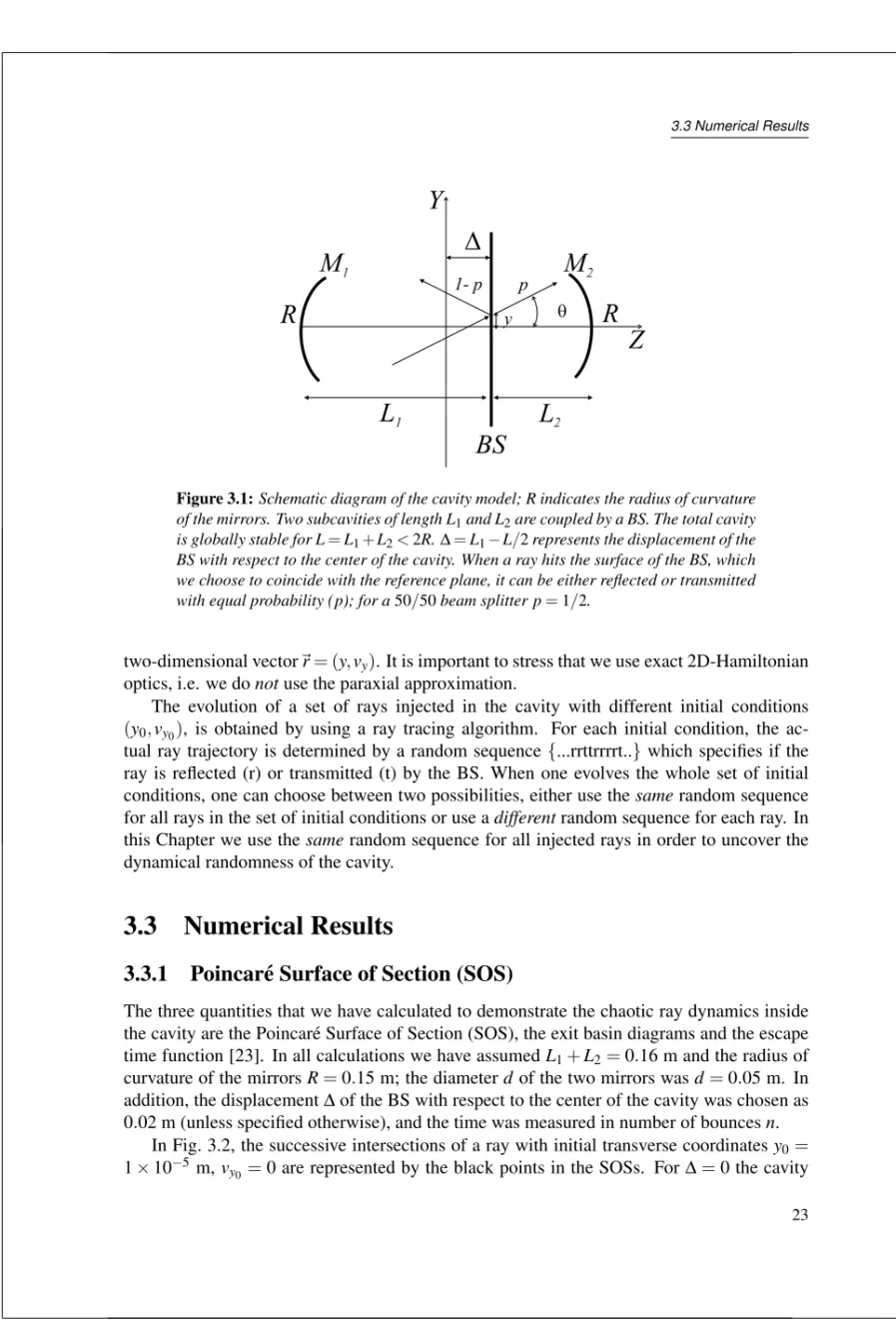
unstabledepending on its geometrical configuration [5]. If a light ray is injected inside the cavity it will remain confined indefinitely when the configuration is stable but it will escape after a finite number of bounces when the cavity is unstable. Our interest is in a cavity which has both aspects of stability and instability (Fig. 3.1). The cavity is modelled as a strip resonator [5] made of two identical concave mirrors of radius of curvatureRseparated by a distanceL, whereL<2Rso that the cavity is globally stable. We then introduce a beam splitter (BS) inside the cavity, oriented perpendicular to the optical axis. In this way the BS defines two planar-concave subcavities: one on the left and one on the right with respect to the BS, with lengthL1andL2, respectively. The main idea is that depending on the position

of the BS the left (right) subcavity becomesunstablefor the reﬂected rays whenL1(L2) is

bigger thanR, while the cavity as a whole remains alwaysstable(L1+L2<2R).

Consideration of this system raises the nontrivial question whether there will be an ”equi-librium” between the number of trapped rays and escaping rays. The trapped rays are those which bounce for infinitely long times due to the global stability of the cavity and the es-caping ones are those which stay only for a finite time. If such equilibrium exists it could eventually lead to transient chaos since it is known in literature that instability (positive Lya-punov exponents) and mixing (confinement inside the system) form the skeleton of chaotic dynamics [22]. In this Chapter we show that under certain conditions such equilibrium can be achieved in our cavity and that chaotic ray dynamics is displayed.

3.2 Our model

In our system the BS plays a crucial role. It is modelled as a stochastic ray splitting element by assuming the reflection and transmission coefficients as random variables [18]. Within the context of wave optics this model corresponds to the neglect of all interference phenom-ena inside the cavity, as required by the ray (zero-wavelength) limit. The stochasticity is implemented by using a Monte Carlo method to determine whether the ray is transmitted or reflected [18]. When a ray is incident on the ray splitting surface of the BS, it is either trans-mitted through it, with probabilityp, or reflected with probability 1−p, where we assume

p=1/2 for a 50/50 beam splitter as shown in Fig. 3.1. We then dynamically evolve a ray and at each reﬂection we use a random number generator with a uniform distribution to randomly decide whether to reﬂect or transmit the incident ray.

(29)

3.3 Numerical Results

Z

p

1- p

BS

q

L

M

R

Y

D

y

Figure 3.1:Schematic diagram of the cavity model; R indicates the radius of curvature of the mirrors. Two subcavities of length L1and L2are coupled by a BS. The total cavity is globally stable for L=L1+L2<2R.Δ=L1−L/2represents the displacement of the BS with respect to the center of the cavity. When a ray hits the surface of the BS, which we choose to coincide with the reference plane, it can be either reﬂected or transmitted with equal probability (p); for a50/50beam splitter p=1/2.

two-dimensional vectorr= (y,vy). It is important to stress that we use exact 2D-Hamiltonian

optics, i.e. we donotuse the paraxial approximation.

The evolution of a set of rays injected in the cavity with different initial conditions

(y0,vy0), is obtained by using a ray tracing algorithm. For each initial condition, the

ac-tual ray trajectory is determined by a random sequence{...rrttrrrrt..} which speciﬁes if the ray is reﬂected (r) or transmitted (t) by the BS. When one evolves the whole set of initial conditions, one can choose between two possibilities, either use thesamerandom sequence for all rays in the set of initial conditions or use adifferentrandom sequence for each ray. In this Chapter we use thesamerandom sequence for all injected rays in order to uncover the dynamical randomness of the cavity.

3.3 Numerical Results

3.3.1 Poincar´e Surface of Section (SOS)

The three quantities that we have calculated to demonstrate the chaotic ray dynamics inside the cavity are the Poincar´e Surface of Section (SOS), the exit basin diagrams and the escape time function [23]. In all calculations we have assumedL1+L2=0.16 m and the radius of

curvature of the mirrorsR=0.15 m; the diameterd of the two mirrors wasd=0.05 m. In addition, the displacementΔof the BS with respect to the center of the cavity was chosen as 0.02 m (unless speciﬁed otherwise), and the time was measured in number of bouncesn.

In Fig. 3.2, the successive intersections of a ray with initial transverse coordinatesy0=

1×10−5_m, _v

(30)

configuration is symmetric and the dynamics is completely regular (Fig. 3.2 (a)); the on-axis trajectory represents an elliptic fixed point and nearby stable trajectories lie on continuous tori in phase space. In Fig. 3.2 (b), the BS is slightly displaced from the center (Δ=0.02 m), the same initial trajectory becomes unstable and spreads over a finite region of the phase space before escaping after a large number of bounces (n=75328). In view of the ring structure of Fig. 3.2 (b) we may qualify the motion as azimuthally ergodic. The fact that the ray-splitting mechanism introduced by the BS produces ergodicity is a well known result for a closed billard [18]. We find here an analogue phenomenon, with the difference that in our case the trajectory does not explore uniformly but only azimuthally the available phase space, as an apparent consequence of the openness of the system.

y

v

( a )

_{( b )}

y

-1x10

1x10

0

0 1x10

-1x10

0 1x10

1.5x10

-1.5x10

0

Figure 3.2:SOS for (a)Δ=0: the ray dynamics is stable and thus conﬁned on a torus in phase space. (b)Δ=0.002m, the dynamics becomes unstable and the ray escapes after n=75328bounces. Note the ring structure in this plot.

3.3.2 Exit basin diagrams

It is well known that chaotic hamiltonian systems with more than one exit channel exhibit irregular escape dynamics which can be displayed, e.g., by plotting the exit basin diagram [24]. In our system, this diagram was constructed by deﬁning a ﬁne grid (2200×2200) of initial conditions(y0,vy0). Each ray is followed until it escapes from the cavity. When

it escapes from above (v_y>0) we plot a black dot in the corresponding initial condition, whereas when it escapes from below (vy<0) we plot a white dot. This is shown in Fig. 3.3,

(31)

3.3 Numerical Results

of chaotic scattering systems [26].

v

_y0

Zoom

0.36

-0.36 0

0.025 -0.025 0

0.09

-0.09

0.00625 -0.00625

0

y

₀

v

_y0

Figure 3.3:Exit basin forΔ=0.02m. The fractal boundaries are a typical feature of chaotic scattering systems.

3.3.3 Escape time function

Besides sensitivity to initial conditions, another fundamental ingredient of chaotic dynamics is the presence of inﬁnitely long living orbits which are responsible for the mixing properties of the system. This set of orbits is usually called repeller [27], and is fundamental to gener-ate a truly chaotic scattering system. To verify the existence of this set we have calculgener-ated the escape time or time delay function [28] for a one-dimensional set of initial conditions speciﬁed by the initial positiony0(impact parameter) taken on the mirrorM1and the initial

velocityvy0 =0. The escape time was calculated in the standard way, as the time (in number

of bouncesn) it takes a ray to escape from the cavity.

(32)

0.0028 0.004 1x105 ( d )

0

( b )

0.0015 0.004 12x104

0 -0.02 0 0.02 0

8x104

( a )

( c )

0.0015 0.0028 14x104

y0(m)

0 Esca pe T ime (bounces) Esc ape T im e (bounces)

y0(m)

Figure 3.4: (a) Escape time as a function of the initial condition y0. (b) Blow up of a small interval along the horizontal axis in (a). (c) and (d) Blow ups of consecutive intervals along the set of impact parameters y0shown in (b).

existence of new infinitely long living orbits. Infinite delay times correspond to orbits that are asymptotically close to an unstable periodic orbit. If we would continue to increase the resolution we would find more and more infinitely trapped orbits. The repeated existence of singular points is a signature of the mixing mechanism of the system due to the global stability of the cavity.

3.4 Summary

(33)

3.4 Summary

(34)

(35)

CHAPTER

4

Universality in the polarization entropy and depolarizing

power of light scattering media: Theory

(36)

4.1 Introduction

In classical optics, a light beam is said to be polarized when its polarization direction de-scribes a stationary curve during the measurement time, and depolarized when its polariza-tion direcpolariza-tion varies rapidly with respect to other degrees of freedom that are not resolved during the experiment, such as wavelength, time or position of the beam [4]. Moreover, de-polarization also occurs when a single-mode input beam is coupled to a multi-mode (either spectral or spatial) optical system and the polarization properties of the outgoing beam are measured with a mode-insensitive device. The main mechanism of depolarization that we analyze in this Chapter is given by the coupling of polarization with spatial degrees of free-dom. A typical example of this is the case of a beam of light initially prepared in a single spatial-mode (kin) that is incident on an optically passive inhomogeneous medium. Due to the

spatial inhomogeneities in the medium, the beam suffers multiple scattering and, as a result, it emerges as a (partially) incoherent superposition of spatial modes (kout). Even when each

of the output modes is fully polarized, the output beam appears to be (partially) depolarized when its spatial information is averaged out in a multi-mode detection set-up.

There exist several formalisms that enable to represent the polarization state of light. Among them, the Mueller-Stokes formalism is particularly well suited for the description of partially polarized light. Within this formalism, the polarization state of the light ﬁeld is completely characterized by the 4 dimensional Stokes vectorS= (S0,S1,S2,S3), where

S0is to the total intensity of the beam, andSi=1,2,3 are the relative intensities in theV/H,

45◦/−45◦, and RHC/LHCbases. The only restriction for a Stokes vector to represent a physical polarization state is that_∑_iS2_i ≤S2₀. Additionally, any passive optical system can be characterized by a 4×4 Mueller matrix, whose 16 real elements map the polarization state of the input and output beams. At this point, it might be good to stress that there exists a considerable ambiguity in the terminology used to characterize different scattering systems; this ambiguity arises from to the overlap of scientiﬁc communities working in the polarimetric properties of light. We specify that in this contribution we will use the standard notation in optics introduced by L. Mandel and E. Wolf [45]. This means, we shall consider as scattering system, any passive optical system that can be characterized by a Mueller matrix (or scattering matrix). In other words, any medium that transforms an input Stokes vectorSininto an output

Stokes vectorSout, provided that the transformation is linear. Thus, the ensemble of scattering

media may comprise a single element, such as a lens, a polarizer, a retarder, a spatial light modulator, or an optical ﬁber, as well as a cascade of optical elements or a solution of micro-particles. These different media may be grouped in two broad classes: deterministic and

non-deterministic[45]. To the ﬁrst class belong all media that do not depolarize the input light, in this particular case, the Mueller matrix representing the medium is a Mueller-Jones matrix [46]. To the second class belong all media that do indeed depolarize the input light and whose Mueller matrix has to be written as a sum of (at most) four Mueller-Jones matrices [46].

For a given depolarizing mechanism, the amount of depolarization can be quantiﬁed by calculating either the entropy (EF) or the degree of polarization (PF) of the scattered ﬁeld [4].

It is possible to show that the ﬁeld quantitiesEF andPF are related by a monotonous

single-valued function. For example, polarized light (PF=1) hasEF =0 while partially polarized

(37)

4.2 Mueller-Stokes formalism

existence of a strongly (weakly) polarized structure in the light ﬁeld [47]. When the incident beam is purely polarized and the output beam is partially polarized, the medium is said to be depolarizing. Depolarization is called isotropic when the degree of polarization 0≤P_F <1 of the scattered ﬁeld is the same for any input pure statePF =1 [48]. In this particular

case, the medium can be characterized by a single parameter, related to the magnitude of its depolarizing power. However, most media depolarize in different amounts different input states of polarization. When this is the case, they are termed anisotropic depolarizers and a single parameter can not fully characterize them. An average measure of the depolarizing power of a medium is given by the so called index of depolarizationDM [49], where the

average refers to different pure input states. Non-depolarizing media are characterized by

DM=1, while depolarizing media have 0≤DM<1.

A depolarizing scattering process is always accompanied by an increase of the entropy of the light, the increase being due to the interaction of the field with the medium, which couples the polarization degrees of freedom of the field with the multi-dimensional degrees of freedom of the scatterer (either spatial or temporal). These extra degrees of freedom are traced over during the polarization measurement, and leave the polarization degrees of freedom of the scattered field in a (partially) mixed state. In general, for an anisotropic depolarizer the entropy added to the light field by the medium will depend on the input state. An average measure of the entropy that a given random medium can add to the entropy of the incident light beam, is given by the polarization entropyEM [48], where the average again refers to

different pure polarization input states. Non-depolarizing media are characterized byEM=0,

while depolarizing media satisfy 0<EM≤1. As the ﬁeld quantitiesEFandPFare related to

each other, so are the medium quantitiesEMandDM, with the main difference that they are

related through amulti-valuedfunction, the reason being that the corresponding relation for the ﬁeld parameters is non-linear.

In Ref. [50] it was shown that there exists a universal relationEM(DM)between the

po-larization entropyEM and the index of depolarizationDM valid for any scattering medium.

More speciﬁcally,EMis related toDMby a multi-valued function which covers the full range

from zero to total depolarization. This universal relation provides a simple characterization of the polarization properties ofanymedium. We emphasize that the results found in [50] apply both to classical and quantum (single photon) scattering processes, and might therefore become relevant for quantum communication optical applications, where depolarization is associated with the loss of quantum coherence [51].

In the next section we review the Mueller-Stokes formalism, suitable for a single spatial mode description of the light ﬁeld. In particular we formally introduce the concepts of deter-ministic and non-deterdeter-ministic Mueller matrices, which correspond to non-depolarizing and depolarizing media respectively.

4.2 Mueller-Stokes formalism

(38)

satisfy theparaxialapproximation. Let

Ex(x,y,z0,t0)≡E0(x,y)e−iω(t0−z0/c), Ey(x,y,z0,t0)≡E1(x,y)e−iω(t0−z0/c), (4.1)

be the components of the complex paraxial electric ﬁeld vector in thex- and y-direction respectively, at the point(x,y)located in the transverse planez=z0at timet0. If the ﬁeld is

uniformon the transverse plane, thenExandEyare independent ofxandy, and a complete

description of the ﬁeld can be achieved in terms of a doubletEof complex variables (with possibly stochastic temporal ﬂuctuations):

E=

E0

E1

, (4.2)

whereE0andE1are now complex-valued functions ofz0andt0only (the subscripts 0 and 1

correspond to the cartesian directionsxandyrespectively). A complete study of the propaga-tion ofEalongzcan be found in [45]. However, the main result we need is that propagation through non-depolarizing media can be described by adeterministic Mueller (or Mueller-Jones) matrixMJ, while to describe the propagation of a light beam through a depolarizing medium it is necessary to use anon-deterministicMueller matrixM.

4.2.1 Deterministic Mueller matrix

M

J

: non-depolarizing media

In a broad sense, adeterministiclinear scatterer as, e.g., a quarter-wave plate, a rotator or a polarizer, is an optical system which can be described by a 2×2 complex Jones [4] matrix

T =

T00 T01

T10 T11

. (4.3)

By this we mean that ifEandEdescribe the polarization state of the ﬁeld immediately before and immediately after the scatterer respectively, then they are linearly related by the Jones matrixT:

E=TE. (4.4)

Therefore a deterministic scattering process, where there are no fluctuations ofE with respect to other degrees of freedom (either spatial or temporal), can be described by a Jones matrix. To account for the possible fluctuations of the field, we can introduce the coherency matrix of the fieldJdefined as [6]

Ji j=EiE∗j, (i,j=0,1), (4.5)

where the angular brackets denote the statistical average over different realizations of the fluctuations of the field. The coherency matrix is Hermitian and positive semi-definite by construction. By imposing as normalization condition Tr{J}=1,Jcan be interpreted as a quantum density matrix [53]; which evidences the analogy between the classical description of a partially polarized beam with the quantum description of a single photon in a mixed state [50]. Given the coherency or covariance matrixJone can calculate the entropy of the fieldEFthrough [4]

(39)

4.2 Mueller-Stokes formalism

where the symbol Tr{·}denotes the trace operation, and 0≤EF ≤1 by deﬁnition. From

Eq. (4.6) we see thatEFis equivalent to the von Neumann deﬁnition of entropy of a

single-photon state [54].

An alternative description can be given in terms of the Stokes parameters of the beam. The four Stokes parametersS_μ (μ=0,...,3)of the beam are deﬁned as

S_μ=Tr{Jσ_μ}, (μ=0,...,3), (4.7) where the{σ_μ}are the normalized Pauli matrices:

σ0=√1₂

1 0

0 1

, σ1=√1₂

0 1

1 0

,

σ2=√1₂

0 −i

i 0

, σ3=√1₂

1 0

0 −1

.

(4.8)

Now, if withS_μ andS_μwe denote the Stokes parameters of the beam before and after the scatterer respectively, it is easy to show that they are linearly related by the real-valued 4×4 Mueller-Jones matrixMJas

S_μ=MJ_μνS_ν, (4.9)

where summation on repeated indices is understood and

MJ=Λ†(T⊗T∗)Λ, (4.10)

where the symbol “⊗” denotes the outer matrix product and theunitarymatrixΛis deﬁned as

Λ=√1 2

⎛ ⎜ ⎜ ⎝

1 0 0 1

0 1 −i 0

0 1 i 0

1 0 0 −1

⎞ ⎟ ⎟

⎠. (4.11)

The columns ofΛare given by the elements of the Pauli matrices. From the structure of

MJit follows that a deterministic medium does not depolarize, that isPF(S) =PF(S)where

the degree of polarizationPFof the ﬁeld is deﬁned as

PF(S) =

S2

1+S22+S23

S0 .

(4.12) By writing the coherency matrixJin terms of the Stokes parameters, and imposing the normalization condition Tr{J}=1, it is possible to show that the degree of polarizationPFis

related to the entropy of the ﬁeldEFby (see Fig. 4.1): EF=−

1+PF

2 log2( 1+PF

2 )− 1−PF

2 log2( 1−PF

2 ). (4.13)

Let us conclude by noticing that for deterministic media the two descriptions in terms of

Classical and quantum scattering in optical systems