Inducing Herding with Capacity Constraints
∗
Alexei Parakhonyak
†and Nick Vikander
‡April 2018
Abstract
We show that a firm may benefit from restricting capacity so as to trigger herding
behavior from consumers, in situations where such behavior is otherwise unlikely. We
con-sider a setting with social learning, where consumers observe sales from previous cohorts
and update beliefs about product quality before making their purchase. A capacity
con-straint directly limits sales but also makes information coarser for consumers, who react
favorably to a sellout because they only infer that demand must exceed capacity. Neither
large cohorts nor unbounded private signals guarantee efficient learning, because the firm
acts strategically to influence the consumers’ learning environment.
JEL classifications: D21, D82, D83
Keywords: social learning, informational herding, cascades, capacity
∗This paper has benefited from discussions with Nemanja Antic, Itai Arieli, Vincent Crawford, Paul Heidhues, Ignacio Monz´on, Steven Morris, David Myatt, Marek Pycia, Gosia Poplawska, Larry Samuelson, Peter Norman Sørensen, Bruno Strulovici, Balazs Szentes, Curtis Taylor, Marta Troya-Martinez, and participants of the Ox-ford Economic Theory Workshop, Game Theory Society World Congress (Maastricht 2016), EARIE (Lisbon, 2016), Transatlantic Theory Workshop 2016, Lancaster Game Theory Workshop 2016, International Industrial Organization Conference (Boston, 2017), and the Royal Economic Society Annual Conference 2018, as well as audiences in Cardiff, Gothenburg, and Copenhagen.
†University of Oxford, Department of Economics and Lincoln College. E-mail: [email protected]
1
Introduction
This paper shows that firms may want to strategically restrict capacity in order to influence
consumer learning, specifically in a way that triggers positive purchase cascades. As is standard
in the literature on social learning (see foundational papers by Banerjee (1992) and Bikhchandani
et al. (1992)), each consumer receives a noisy private signal about product quality, but also infers
some information from observing earlier sales. To illustrate the mechanism at work, consider
ten consumers who visit a firm, where each buys if and only if her signal was good. A consumer
who then arrives and observes initial sales of three may well refuse to buy, even if her own signal
was good, because she infers that only three out of the ten others had a good signal. But if the
firm, without knowing product quality, had initially limited capacity to three sales per period,
then the consumer would observe a sellout, and only infer that there were at least three good
signals. That may well be sufficiently good news for the consumer to buy even if her own signal
was bad. Thus, Sgroi’s (2002) suggestion that the presence of multiple ‘guinea pigs’ who do not
observe others’ choices will help lead to efficient social learning does not hold in our setting,
because the firm uses capacity to manipulate the learning environment.
An alternative way to avoid ‘pathological outcomes’ of social learning where consumers herd
on the wrong action is to have unboundedly informative signals, as proposed by Smith and
Sørensen (2000). Consumers with such signals will effectively ignore public information and
their choices can prevent incorrect cascades. Suppose that in our example, one out of ten
consumers per period is perfectly informed about quality and that the firm in unconstrained. If
quality is low, but say seven consumers in period 1 receive good signals, then everyone will buy in
period 2 except for the informed consumer. But the informed consumer’s choice not to buy will
perfectly reveal that quality is low and lead to zero sales in later periods. Similarly, if quality
is high but seven consumers in period 1 receive bad signals, then the informed consumer’s
choice to buy in period 2 will ensure that everyone buys in later periods. This is not the
case, however, for a firm that restricts capacity. The informed consumer’s action prevents an
to buy is then unobservable; she is effectively pooled with consumers who are rationed.1 The
endogenous information structure means that learning may not occur despite private signals
being unbounded, namely in situations where learning would hurt the firm.
Our focus on sellouts and rationing fits in with evidence of a variety of products where
demand appears to persistently far outstrip supply. Shortages for ‘Beanie Babies’ were
accom-panied by extremely high demand from 1996 to 1999, before the resale market crashed shortly
thereafter.2 For high-end restaurants, tables at ‘Noma’ in Copenhagen remain notoriously
dif-ficult to come by, and reported waiting times for ‘Damon Baehrel’ or ‘Club 33’ in the United
States range from ten to fourteen years. Music festivals, such as those in Roskilde and Reading,
also often sell out well in advance, year after year, with tickets for Glastonbury 2016 selling out
in just 30 minutes.3 Sellouts are also common in professional sports, where the Boston Red Sox
enjoyed a sellout streak which stretched 2003 to 2013.
Formally, we consider a model of social learning where cohorts of consumers arrive
sequen-tially at a seller and observe sales from all previous periods. Informed consumers perfectly know
whether product quality is high or low, whereas uninformed consumers receive a private noisy
signal. Consumers in each cohort simultaneously choose whether to buy or take their outside
op-tion and then leave the game. Initially, without knowing its quality, the seller can set a capacity
constraint, where per period sales cannot exceed capacity. This constraint effectively coarsens
the information of consumers, since they cannot observe the extent of any excess demand.
We show that the seller may find it strictly profitable to restrict capacity even though the
constraint directly limits sales in each period. The reason is that sellouts drive up uninformed
consumers’ willingness to pay, and can generate positive purchase cascades where they all want
to buy regardless of their signal. The result is high sales and excess demand in later periods. This
1In the spirit of Smith and Sørensen (2000), we use the word ‘cascade’ to refer to a situation where all
consumers with boundedly informative signals take the same action regardless of their private information.
2Debo et al. (2012) argue that scarcity in the case of Beanie Babies was largely due to seller strategic behaviour.
See also: https://nypost.com/2015/02/22/how-the-beanie-baby-craze-was-concocted-then-crashed/, accessed on April 2, 2018.
3See http://www.glastonburyfestivals.co.uk/glastonbury-2016-tickets-sell-out-in-30-minutes/, accessed on
excess demand can actually benefit the seller, if quality is in fact low, by masking the actions
of informed consumers who choose not to buy, thereby allowing the cascade to be maintained.
Indeed, we show that restricting capacity tends to be optimal in situations that a priori seem
grim: when quality is likely low, and signals are quite accurate.
Our paper contributes to the literature on social learning where agents cannot all perfectly
observe each other’s actions. Different work in this literature has assumed that agents can
ob-serve a random sample of earlier actions that is anonymous (Banerjee and Fudenberg (2004),
Smith and Sorensen (2013), Monz´on and Rapp (2014), Monz´on (2017)) or non-anonymous
(Ace-moglu et al. (2011), Lobel and Sadler (2015)), the aggregate total of all past actions (Callander
and H¨orner, 2009), the aggregate total of one particular action (Herrera and H¨orner (2013),
Guarino et al. (2011)), or only the choice of an agent’s immediate predecessor (C¸ elen and Kariv,
2004). In all these cases the information structures is exogenous. In our paper, it is the firm’s
strategic choice of information structure that prevents consumers from learning about low
qual-ity, despite our setting having two features that the literature suggests should promote learning:
multiple consumers who do not have access to social information (see Banerjee (1992), Sgroi
(2002), Acemoglu et al. (2011), Smith and Sorensen (2013), Golub and Sadler (2017)); and
unbounded private signals (see Smith and Sørensen (2000), Banerjee and Fudenberg (2004),
amongst many others).
Our paper also relates to recent work that considers how an uninformed designer can choose
an information structure for agents in order to influence social learning. Kremer et al. (2014)
and Che and Horner (2015) both consider settings where agents arrive sequentially, and show
that a designer looking to maximize total surplus may prefer an information structure that is
coarse. Coarse information can encourage agents to experiment which can help them learn from
one another.4 In contrast, we consider a firm looking to maximize profits, and show that it may
choose a coarse information structure in order to limit learning.
The idea that an uninformed seller may design an information structure to persuade agents
4Smith et al. (2017) analyze a setting with social learning from a social planner’s perspective, and also argue
over time also plays a central role in work on dynamic Bayesian persuasion, in which a designer
can conduct statistical experiments, the results of which reveal information about the unknown
state to a decision maker (or decision makers) (see Au (2015), Ely (2017), Renault et al. (2017),
Best and Quigley (2017), Bizzotto et al. (2018), Orlov et al. (2018)). Bizzotto et al. (2018) and
Orlov et al. (2018) both assume the decision-maker can also learn an alternative sources, namely
from exogenous public news, but not from the actions of other players; as in the rest of this
literature, there is no social learning.
The literature on how firms can influence consumer learning about product quality has
mainly focused on pricing (Welch (1992), Bose et al. (2006), Bose et al. (2008), Sayedi (2018)),
although some work has considered strategic scarcity.5 Debo et al. (2012) show that a firm
may reduce service speed so that consumers observe longer queues, since long queues suggest
high quality. In Stock and Balachander (2005), a firm can set low inventory, which consumers
then observe and believe that demand (and quality) is high. Both papers assume the firm is
privately informed about quality, and can potentially use this information to mislead consumers.
Moreover, in contrast to our work, scarcity does not hide information from consumers in these
settings, but instead may actually help reveal it.6
We describe our model in section 2, present our analysis in section 3, and section 4 then
concludes. All the proofs are presented in web-appendix A, and web-appendix B provides a
general characterization of the profit function of a capacity constrained firm.
5See also Gill and Sgroi (2008) on product testing, Gill and Sgroi (2012) on choice of reviewers, and Aoyagi
(2010), Liu and Schiraldi (2012), and Bhalla (2013) on simultaneous versus sequential product launch.
6Vikander (2017) considers a fully informed firm that may limit capacity to influence consumer beliefs, but
2
Model
Suppose there is a product or service of unknown quality and two possible states of the world,
Ω ={G, B}. In state G, quality is good and each consumer who buys obtainsuG = 1. In state
B, quality is bad and each consumer who buys obtains uB = 0. A consumer who does not buy
gets reservation utility r ∈(0,1).
The actual state of the world is known neither to the seller nor to consumers at the start
of the game. A priory beliefs of all players are that P(G) ≡ β and P(B) = 1−β. In each
period there are 2npotential buyers, who are eitherinformed oruninformed. Before making her
purchase decision, each informed consumer receives a signal that reveals the state for sure. Each
uninformed consumer receives a noisy private signal, s∈ {g, b}, where P(g|G) = P(b|B)≡α∈
(1/2,1). We assume α < 1, so our signals are boundedly informative, and a consumer without
further information would follow her signal, i.e. P(G|s =g)> r > P(G|s =b). We model the
number of informed consumers in two ways. In thedeterministic setting, we will assume there
is a fixed number m < nof informed consumers in every period. In the stochastic setting, we
will assume that each of the 2n consumers can be informed with probabilityε.7
The timing of the model is as follows. At the start of the game, t = −1, the seller can
set a capacity constraint K ≤ 2n. This capacity choice is irreversible and limits potential sales
in each period (i.e. how many consumers can buy), which cannot exceed capacity. The state
of the world is realized at t = 0, which implies that the constraint itself does not reveal any
information.8
In each period t ∈ [1,∞), 2n consumers arrive and observe both capacity and total sales
7Our approach of modeling unboundedly informative signals, through the presence of fully informed
con-sumers, differs from that usually taken in the literature, which instead assumes continuous signals. Our approach helps with tractability and allows us to write down explicit expressions for profits, whereas the traditional ap-proach typically only provides results about learning in the limit.
8Parsa et al. (2005) document that about 60% of new restaurants fail within three years, which suggests that
from the consumers in previous cohorts. That is, consumers do not directly observe quantity
demanded in the each period, but only quantity sold. Notice that a sellout in period t0 < t,
where sales equal capacity, need not imply that demand precisely equaled capacity. Thus, a
capacity constraint can potentially limit the information available to consumers about each
others’ behaviour.
Each of the 2n consumers who arrive in period t choose whether they want to buy based
on (i) prior beliefs about quality, β, (ii) a private signal, s, and (iii) observed sales from the
previous cohorts.9 The decision of informed consumers is solely determined by their signal. If
more than K consumers want to buy in period t, a random selection of them are served, and
the remaining consumers use their outside option. All period-tconsumers then leave the market
forever, and a new cohort of 2n consumers arrives in periodt+ 1.
The seller receives a fixed profit per consumer who buys, normalized to 1. He discounts
profits in future periods with a factor of δ, and sets K so as to maximize expected discounted
future profits.
3
Analysis
3.1
Consumer Behaviour
DefineQiω(j) as the probability ofj good signals from 2n consumers in period 1, conditional on the state being ω ∈ {G, B} , in either the deterministic (denote i =det) or stochastic (denote
i=sto) setting. In the deterministic setting,m consumers receive a correct signal for sure, and
the remaining 2n−m consumers each receive a correct signal with probability α, which implies
QdetG (j) =
2n−m j −m
αj−m(1−α)2n−j, (1)
9In our setting it does not matter how long a history is observed, provided that consumers observe at least
if j ≥m, and QdetG (j) = 0 if j < m, along with
QdetB (j) =
2n−m j
α2n−m−j(1−α)j, (2)
if j <2n−m and zero otherwise.
In the stochastic setting, each consumer receives a correct signal with probability+(1−)α,
where is the probability of being informed. This implies:
QstoG (j) =
2n j
[1−(α+ε−αε)]2n−j(α+ε−αε)j, (3)
QstoB (j) =
2n j
[1−(α+ε−αε)]j(α+ε−αε)2n−j. (4)
We start by showing that Qi
ω(j) satisfies the following four properties.
Lemma 1. Both in the deterministic and stochastic settings,Qi
ω(j), ω ∈ {G, B}, i∈ {det, sto},
we have:
(i) QiB(j)
Qi G(j)
is non-increasing in j.
(ii) QiB(n)
Qi G(n)
= 1, QiB(n−1)
Qi G(n−1)
≥ α
1−α
2
and QiB(n+1)
Qi G(n+1)
≤ 1−α α
2 .
(iii) Qi
B(j) =QiG(2n−j) for all j ≤2n.
(iv) Qi
G(j)> QiG(2n−j) if j ≥n+ 1.
That is, (i) more good signals means the good state is more likely, (ii) an equal number of
good and bad signals means both states are equally likely, and the smallest difference from an
equal number is sufficiently informative about the state, (iii) j good signals in the bad state is
as likely as j bad signals in the good state, and (iv) in the good state, j ≥n+ 1 good signals is
more likely than j bad ones.
Now we formulate the optimal behaviour for a consumer in period tfacing an unconstrained
seller, following a sequence of sales (S1, . . . , St−1).
Lemma 2. Suppose the seller is unconstrained and consider an uninformed consumera acting
1. If S1 =. . . St−2 =n and
(a) if St−1 > n then a buys regardless of her own signal;
(b) if St−1 =n then a follows her own signal;
(c) if St−1 < n then a does not buy regardless of her own signal.
2. If maxτ≤t−2Sτ > n and
(a) if St−1 = 2n, then a buys regardless of her own signal;
(b) if St−1 <2n then a does not buy regardless of her own signal.
3. If maxτ≤t−2Sτ < n and
(a) if St−1 >0, then a buys regardless of her own signal;
(b) if St−1 = 0 then a does not buy regardless of her own signal.
Following the literature on social learning, Lemma 2 describes optimal behavior on the
equilibrium path; we not specify consumers’ beliefs and best responses for histories which cannot
arise from equilibrium behaviour. As each consumer’s payoff does not depend on the actions of
those who follow, this approach is not restrictive. The idea of Lemma 2 is that initial sales of
at leastn+ 1 out of 2n is sufficiently good news to trigger a positive purchase cascade where all
uninformed consumers buy. This cascade continues unless (or until) there is a period with fewer
than 2n sales, which would reveal that an informed consumer chose not to buy, and that the
state was actually bad. This would in turn trigger a negative cascade. The story is similar for
sales of at mostn−1 in period 1, which triggers a negative cascade where uninformed consumers
do not buy, unless (or until) where is a period with strictly positive sales.
Now we look into consumer behaviour when the seller restricts capacity. It follows from
Lemma 2 that a seller should only consider setting K ≤ n, as larger capacity limits sales
compared to being unconstrained, but does not increase the probability of a positive cascade.
Moreover, setting capacity very low means that multiple sellouts may be necessary to trigger
has very little impact on consumers’ beliefs. However, as Lemma 3 establishes, consumers
become increasingly optimistic after each sellout, so that sufficiently many sellouts will trigger
a cascade.
Consider a consumer in cohort l+ 1 who receives a bad signal, realizes there were sellouts in
alll previous periods, and believes that all earlier consumers followed their private signals. Let
γ(l, K) denote this consumer’s belief that the state is good. Then:
γ(l, K) = P(G∩b, lsellouts)
P(G∩b, l sellouts) +P(B∩b, l sellouts) =
β(1−α)
h P2n
j=KQ i G(j)
il
β(1−α)
h P2n
j=KQiG(j)
il
+ (1−β)α
h P2n
j=KQiB(j)
il =
1
1 + 1−ββ1−αα
hP2n j=KQiB(j) P2n
j=KQiG(j)
il (5)
where i∈ {det, sto}.
Lemma 3. Both in the deterministic and stochastic settings, for all 1 ≤ K ≤ n, consumer
beliefs γ(l, K) are increasing in l, with liml→∞ γ(l, K) = 1.
As beliefs γ(l, K) are increasing inl, a sequence of sell-outs will eventually lead to a positive
purchase cascade. Moreover, for all parameter values satisfying our assumptions, there is always
a value of the outside optionr such that a single sell-out triggers such behavior.
Lemma 4. For all K ≤n there existsr ∈(0,1)such that γ(1, K)> r > γ(0, K) =P(G|s =b).
We will apply Lemma 4 for establishing our main result, i.e. that for some parameter values
the seller prefers to restrict capacity. The general profit function, without assuming that one
sell-out is sufficient to trigger a cascade, is presented in Appendix B.10
10There we illustrate that a seller might sometimes prefer delaying a cascade by setting low capacity. As
3.2
Sellers
Our aim is to show that there is a range of parameters both in the stochastic and the deterministic
settings such that the seller wants to restrict its capacity. Moreover, we show that each value of
K ≤n can sometimes lead to higher profit than remaining unconstrained. We start our analysis
with the following preliminary result. Let Q = {Q(j), 0 ≤ j ≤ 2n} be a discrete probability
measure: Q(j) ∈ [0,1] and P2n
j=0Q(j) = 1. At this point we are agnostic about the actual probabilistic model, so we do not use model superscipts. Define functions
πuQ = 1 1−δQ(n)
2n
X
j=0
jQ(j) + 2nδ 1−δ
2n
X
j=n+1
Q(j)
!
, (6)
where δ∈(0,1).
πcQ(K) = 2n
X
j=0
min{j, K}Q(j) + Kδ 1−δ
2n
X
j=K
Q(j). (7)
Equations (6)-(7) define seller profits assuming that cascades, once started, continue forever.
This is true in the deterministic setting with m = 0 and the stochastic setting with ε = 0.
Here, however, we allow Q to be a fairly arbitrary probability measure. The following Lemma
shows that if probabilitiesQare chosen in a particular way, the seller prefers to be constrained,
provided that cascades continue forever. Later, in the proofs of the corresponding theorems, we
will show that (i) parameters of the model can be chosen such that Qi(j), i∈ {det, sto} satisfy
the properties required by Lemma 5 and (ii) the assumption that cascades continue forever
understates the seller’s incentive to restrict capacity.
Lemma 5. Consider a sequence of probability measures {Qs}∞
s=0 such that lims→∞ Q
s(n) P2n
j Qs(j)
=
∞. Then, there exist δ and T0, such that for all s > T0, n >1, K ≤n
πuQs < πcQs(K)
Moreover, if lims→∞Qs(n) = 0 there is a sufficiently large T1 such that for all s > T1 the
inequality πuQs < πQcs(K) holds for all δ∈q2n−K
2n ,1
.
Now we are ready to provide a formal analysis of seller’s incentives to restrict capacity. We
signal and the state is good, or where all uninformed consumers refuse to buy regardless of their
signal and the state is bad. We define an incorrect cascade as a situation where all uninformed
consumers refuse to buy and the state is good, or where all uninformed consumers buy and the
state is bad.
We start with the deterministic model. The profit of an unconstrained seller is
πudet= 2n
X
j=0
jQdet(j) +δQdet(n)πdetu
+βδ
" 2n X
j=n+1
QdetG (j) 2n 1−δ +
n−1
X
j=0
QdetG (j)
m+Im≥1 2nδ
1−δ
#
+ (1−β)δ
" 2n X
j=n+1
QdetB (j) 2n 1−δ −
2n
X
j=n+1
QdetB (j)
m+Im≥1 2nδ
1−δ
#
(8)
whereIis an indicator function. For an unconstrained seller, period-1 sales of more (less) thann
immediately trigger a positive (negative) cascade. This cascade continues for all further periods
if it is correct, but not if it is incorrect and some consumers are informed. An incorrect cascade
will then be reversed in period 2 as informed consumers’ purchase decisions reveal the true state.
The result is a correct cascade in all future periods.
According to Lemma 4, there are values of r for which a single sell-out generates a cascade.
For such values of r, the profit of a seller with capacity constraint K is
πcdet(K) = 2n
X
j=0
min{j, K}Qdet(j)
+βδ
" 2n X
j=K
QdetG (j) K 1−δ +
K−1
X
j=0
QdetG (j)
min{m, K}+Im≥1
Kδ
1−δ
#
+ (1−β)δ
" 2n X
j=K
QdetB (j) K 1−δ
#
. (9)
One difference with (9) compared to (8) is that period-1 sales of more (less) thanK now trigger
be reversed, even though informed consumers refuse to buy in every period. Their decisions are
effectively hidden by the capacity constraint, as they are pooled with uninformed consumers
who are rationed.
Theorem 1. For any n > 1, 0 ≤ m < n, K ≤ n and δ >
q
2n−K
2n , there are (α, β) ∈
(1/2,1)×(0,1/2) and r >0 for which the seller can increase its profit above the unconstrained
level by restricting capacity to K.
This result is proved in two steps. First, if the seller is unconstrained, then informed
con-sumers’ choices will immediately reverse any incorrect cascade, but an incorrect positive cascade
is more likely than an incorrect negative one, because the bad state is more likely. This implies
πdet
u < π
Qdet
u . If the seller is constrained, then informed consumers’ choices will immediately
reverse an incorrect negative cascade, but will never reverse an incorrect positive one, which
implies πdet
c (K)> π
Qdet
c (K). The second step is to show that α and β can be chosen in such a
way that Lemma 5 applies.
Intuitively, restricting capacity can help the seller by increasing the probability of a positive
cascade, and by helping such a cascade, once triggered, to be maintained. This is true in
particular for an incorrect positive cascade where uninformed consumers never learn that quality
is low. The first channel is that restricting capacity makes it more likely that all uninformed
consumers want to buy immediately after observing period-1 sales. Specifically, below average
sales between K and n, are more likely when the state is bad, and can only trigger a positive
cascade if the seller is constrained. Moreover, as described above, the presence of informed
consumers will immediately reverse any incorrect cascade if the seller is unconstrained, but will
not reverse an incorrect positive cascade if the seller is constrained; the decision of uninformed
consumers not to buy is effectively unobservable, as sellouts continue to occur in all periods.
As similar result applies in the stochastic setting. The profit function of an unconstrained
πusto= 2n
X
j=0
jQsto(j) +δQsto(n)πusto
+βδ
" 2n X
j=n+1
QstoG (j) 2n 1−δ +
n−1
X
j=0
QstoG (j)
P2n i=1
2n i
εi(1−ε)2n−i(i+12−nδδ) 1−(1−ε)2nδ
!#
+ (1−β)δ
" 2n X
j=n+1
QstoB (j) 2n 1−δ −
2n
X
j=n+1
QstoB (j)
P2n i=1
2n i
εi(1−ε)2n−i(i+ 12−nδδ) 1−(1−ε)2nδ
!#
. (10)
The profit function of a constrained seller is given by
πcsto(K) = 2n
X
j=0
min{j, K}Qsto(j)
+βδ
" 2n X
j=K
QstoG (j) K 1−δ +
K−1
X
j=0
QstoG (j)
" P2n i=1
2n i
εi(1−ε)2n−i(min{i, K}+ Kδ
1−δ)
1−(1−ε)2nδ
##
+(1−β)δ
" 2n X
j=K
QstoB (j) K 1−δ −
2n
X
j=K
QstoB (j)
" P2n
i=2n−K+1 2n
i
εi(1−ε)2n−i(i−2n+K+ 1Kδ−δ) 1−P2n−K
i=0 2n
i
εi(1−ε)2n−iδ
##
.
(11)
These profits functions resemble those in the deterministic setting, except incorrect cascades
are now eventually corrected, regardless of whether the seller is unconstrained. Incorrect negative
cascades are corrected as soon as a single informed consumer arrives, and the same applies for
incorrect positive cascades if the seller is unconstrained. For a constrained seller experiencing
an incorrect positive cascade, at least 2n−K+ 1 informed consumers must arrive in the same
period and prevent a sellout, in order for the state to be revealed.
Theorem 2. For any n >1, K ≤n and δ >
q
2n−K
2n , there are (α, β, ε)∈(1/2,1)×(0,1/2)×
(0,1) and r > 0 for which the seller can increase its profit above the unconstrained level by
restricting capacity to K.
An important difference with Theorem 1 is that Theorem 2 holds for someε, while Theorem
1 holds for all m ≤ n. This is because in the deterministic setting an appropriately capacity
this is not the case, and an incorrect positive cascade really only pays off if the probability of
having many informed consumers is sufficiently low.
As in the deterministic setting, restricting capacity increases the probability of period-1
sales triggering a positive cascade, and helps prevent such a cascade from being reversed in later
periods if the state is bad. Incorrect positive cascades are eventually corrected, but this take
substantially longer if the seller is constrained. Formally, given an incorrect positive cascade, the
expected number of periods until the bad state is revealed is 1/P, whereP =P2n−K
i=0 2n
i
εi(1−
ε)2n−i if the seller sets capacity constraint K, and P = (1−)2n if the seller is unconstrained.
For example, if 2n = 6 and ε= 0.1, and if initial sales trigger a mistaken positive cascade, then
it requires an average of two periods to reveal the true state if the seller is unconstrained, but
787 periods if K = 3 and about one million periods if K = 1.
Having shown that the seller may sometimes find it profitable to restrict capacity, we now
say something about the conditions under which this can occur.
Proposition 1. Suppose that β ≥1/2. Then the seller should not restrict capacity: πui > πci(K)
for all K and i∈ {det, sto}.
The intuition is that restricting capacity can only pay off in the bad state. When the state is
good, initial sales are likely sufficiently high to trigger a positive cascade regardless of whether the
seller restricts capacity, and an unconstrained seller then enjoys higher sales. The proof shows
that forβ > 12, the good state is sufficiently likely that expected sales for an unconstrained seller
exceed n per period. This is more than the seller could possibly earn per period by restricting
capacity to K ≤n.
The sufficient condition provided in Proposition 1 is simple and intuitive, but the necessary
condition is much harder to obtain, so we investigate this question numerically. Figure 1(a),
where all consumers are informed, shows that the region where restricting capacity can be
optimal is larger when there are many consumers. There is also an interesting interaction
between signal precision and the prior. When the signal is very imprecise (α ≈ 1/2), it is
relatively likely that at least half of consumers will buy, regardless of the state, so the seller will
an unconstrained seller becomes increasingly likely to experience a negative cascade when the
state is bad, so the seller will restrict capacity for sufficiently small β. A further increase in
signal precision makes restricting capacity increasingly helpful in the bad state, but increasingly
harmful in the good state, as a correct positive cascade is then likely without a constraint. The
first effect dominates for intermediate α, but the second effect dominates when α is sufficiently
large, because a mistaken positive cascade is only likely given a very low constraint, which would
dramatically reduce profits in the good state. Figure 1(b) depicts the optimal level of capacity
for these different parameter values.
Figures 1(c) and 1(d) show how informed consumers affect the seller’s incentive to restrict
capacity. They do so indirectly, via the way that m ≥1 or > 0 changes the probabilities Qi ω
and affect how likely a cascade is to be triggered; and also directly, via the way that m ≥ 1
or >0 explicitly enter the profit function, because informed consumers can reverse incorrect
cascades. The gray bell-shaped area shows when restricting capacity is optimal if all consumers
are uninformed. The first channel of having informed consumers shifts the bell shape to the
left (lighter area): more purchase decisions in early cohorts are likely to reflect the true state,
which is analogous to an increase in signal precision. In this area, the inequality πQui < πQci(K) holds for some K. The second channel unambiguously increases the seller’s incentive to restrict
capacity (darker area on top of the lighter one) because a capacity constraint helps prevent
informed consumers from reversing an incorrect positive cascade.
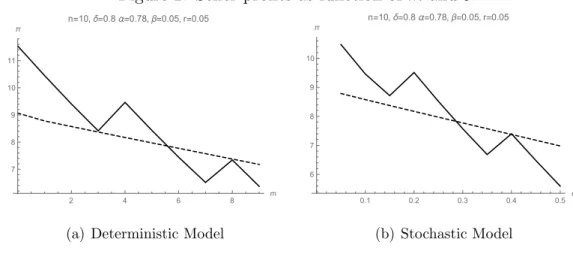
Figure 2 illustrates how profits depend on m and ε. Both the profits functions are directly
decreasing in the number of informed consumers because we here assume thatβ <1/2.
Nonethe-less, the constrained profit function is saw shaped, because more informed consumers can also
reduce the number of sellouts required to trigger a positive cascade. For example, an increase
in m can lead the seller to reduce K, because one sellout can now trigger a cascade at lower
Figure 1: Seller profits and L.
(a) m = 0 or ε= 0, area where constraint is optimal for somer, δ.
(b) OptimalK,m= 0 orε= 0.
Figure 2: Seller profits as function of m and ε.
2 4 6 8 m
7 8 9 10 11 π
n=10,δ=0.8α=0.78,β=0.05, r=0.05
(a) Deterministic Model
0.1 0.2 0.3 0.4 0.5 ϵ
6 7 8 9 10
π
n=10,δ=0.8α=0.78,β=0.05, r=0.05
(b) Stochastic Model
4
Conclusions
In this paper, we show that a firm may benefit from restricting capacity, to trigger herding
behav-ior from consumers and increase future sales. Limiting capacity results in coarser information, as
consumers who observe a sellout attach positive probability to all levels of demand that exceed
capacity. The results show that two main mechanisms the literature suggests may help avoid
pathological social learning outcomes, ‘guinea pigs’ and unbounded private signals, can fail to
do so, if the firm is able to manipulate the learning environment by a simple instrument such
as limiting capacity.
Our results rely on the idea that consumers can observe sales and capacity. This is reasonable
in many markets, e.g. restaurants, sports and concert tickets, and limited car editions, where
sales and capacity are often widely known, but the extent of any excess demand is not. Product
scarcity should also affect learning in other settings, but in a way that depends precisely on
what consumers can observe. For example, it will matter if concert promoters can ‘paper the
house’ by quietly filling seats for free, or if sales figures for certain consumer products become
widely reported precisely because shortages occurred.
In line with most work on social learning, our seller is not privately informed, but an alterative
would be to assume that the seller receives its own private binary signal about quality. The full
signal precision is low, then there can exist an equilibrium where the seller restricts capacity.
Our model can be viewed as a limit case of such a pooling equilibrium where the seller’s signal
is completely uninformative. A separating equilibrium would require that period-1 consumers
always follow their own signal, along with a standard incentive compatibility condition where
the seller only wants to restrict capacity after a bad signal. Notice the connection here with a
key result in our analysis: that it is precisely a seller that expects relatively low sales that can
References
Daron Acemoglu, Munther A Dahleh, Ilan Lobel, and Asuman Ozdaglar. Bayesian learning in
social networks. The Review of Economic Studies, 78(4):1201–1236, 2011.
Masaki Aoyagi. Optimal sales schemes against interdependent buyers. American Economic
Journal: Microeconomics, 2(1):150–82, 2010.
Pak Hung Au. Dynamic information disclosure. The RAND Journal of Economics, 46(4):
791–823, 2015.
Abhijit Banerjee and Drew Fudenberg. Word-of-mouth learning.Games and Economic Behavior,
46(1):1–22, 2004.
Abhijit V Banerjee. A simple model of herd behavior. The Quarterly Journal of Economics,
pages 797–817, 1992.
James Best and Daniel Quigley. Persuasion for the long run. 2017.
Manaswini Bhalla. Waterfall versus sprinkler product launch strategy: Influencing the herd.
The Journal of Industrial Economics, 61(1):138–165, November 2013.
Sushil Bikhchandani, David Hirshleifer, and Ivo Welch. A theory of fads, fashion, custom, and
cultural change as informational cascades. Journal of Political Economy, pages 992–1026,
1992.
Jacopo Bizzotto, Jesper R¨udiger, and Adrien Vigier. Dynamic persuasion with outside
infor-mation. 2018.
Subir Bose, Gerhard Orosel, Marco Ottaviani, and Lise Vesterlund. Dynamic monopoly pricing
and herding. The RAND Journal of Economics, 37(4):910–928, 2006.
Subir Bose, Gerhard Orosel, Marco Ottaviani, and Lise Vesterlund. Monopoly pricing in the
Steven Callander and Johannes H¨orner. The wisdom of the minority. Journal of Economic
theory, 144(4):1421–1439, 2009.
Bo˘ga¸chan C¸ elen and Shachar Kariv. Observational learning under imperfect information.Games
and Economic Behavior, 47(1):72–86, 2004.
Yeon-Koo Che and Johannes Horner. Optimal design for social learning. 2015.
Laurens G Debo, Christine Parlour, and Uday Rajan. Signaling quality via queues.Management
Science, 58(5):876–891, 2012.
Patrick DeGraba. Buying frenzies and seller-induced excess demand. The RAND Journal of
Economics, pages 331–342, 1995.
Jeffrey C Ely. Beeps. American Economic Review, 107(1):31–53, 2017.
David Gill and Daniel Sgroi. Sequential decisions with tests. Games and economic Behavior,
63(2):663–678, 2008.
David Gill and Daniel Sgroi. The optimal choice of pre-launch reviewer. Journal of Economic
Theory, 147(3):1247–1260, 2012.
Benjamin Golub and Evan D Sadler. Learning in social networks. 2017.
Antonio Guarino, Heike Harmgart, and Steffen Huck. Aggregate information cascades. Games
and Economic Behavior, 73(1):167–185, 2011.
Helios Herrera and Johannes H¨orner. Biased social learning. Games and Economic Behavior,
80:131–146, 2013.
Ilan Kremer, Yishay Mansour, and Motty Perry. Implementing the wisdom of the crowd.Journal
of Political Economy, 122(5):988–1012, 2014.
Ting Liu and Pasquale Schiraldi. New product launch: herd seeking or herd preventing?
Ilan Lobel and Evan Sadler. Information diffusion in networks through social learning.
Theo-retical Economics, 10(3):807–851, 2015.
Marc M¨oller and Makoto Watanabe. Advance purchase discounts versus clearance sales. The
Economic Journal, 120(547):1125–1148, 2010.
Ignacio Monz´on. Aggregate uncertainty can lead to incorrect herds. American Economic
Jour-nal: Microeconomics, 9(2):295–314, 2017.
Ignacio Monz´on and Michael Rapp. Observational learning with position uncertainty. Journal
of Economic Theory, 154:375–402, 2014.
Volker Nocke and Martin Peitz. A theory of clearance sales. The Economic Journal, 117(522):
964–990, 2007.
Dmitry Orlov, Andrzej Skrzypacz, and Pavel Zryumov. Persuading the principal to wait. 2018.
HG Parsa, John T Self, David Njite, and Tiffany King. Why restaurants fail. Cornell Hotel and
Restaurant Administration Quarterly, 46(3):304–322, 2005.
J´erˆome Renault, Eilon Solan, and Nicolas Vieille. Optimal dynamic information provision.
Games and Economic Behavior, 104:329–349, 2017.
Amin Sayedi. Pricing in a duopoly with observational learning. 2018.
Daniel Sgroi. Optimizing information in the herd: Guinea pigs, profits, and welfare. Games and
Economic Behavior, 39(1):137–166, 2002.
Lones Smith and Peter Sørensen. Pathological outcomes of observational learning.Econometrica,
68(2):371–398, 2000.
Lones Smith and Peter Norman Sorensen. Rational social learning by random sampling. 2013.
Lones Smith, Peter Norman Sorensen, and Jianrong Tian. Informational herding, optimal
Axel Stock and Subramanian Balachander. The making of a hot product: A signaling
explana-tion of marketers scarcity strategy. Management Science, 51(8):1181–1192, 2005.
Nick Vikander. Sellouts, beliefs, and bandwagon behavior. Mimeo, 2017.
Ivo Welch. Sequential sales, learning, and cascades. The Journal of finance, 47(2):695–732,
1992.
Web-Appendix A
Proof of Lemma 1. Deterministic model. Consider QdetG (j) given by (1) and QdetB (j) given by (2). Clearly, QdetB (j)
Qdet G (j)
= 0 if 2n−j ≤m−1, and for 2n−j ≥m
QdetB (j)
Qdet G (j)
=
(j−m)! (2n−m−j)!
(2n−j)!
j!
α2(n−j)(1−α)2(j−n)
which is decreasing in j and equals to 1 when j =n. Moreover, for j =n−1 we get
Qdet
B (n−1)
Qdet
G (n−1)
= n(n+ 1) (n−m−1)(n−m)
α2 (1−α)2 >
α2 (1−α)2
and for j =n+ 1 we get
Qdet
B (n+ 1)
Qdet
G (n+ 1)
= (n−m−1)(n−m)
n(n+ 1)
(1−α)2
α2 <
(1−α)2
α2
Now,
QdetG (2n−j) =
2n−m
2n−j−m
α2n−j−m(1−α)j =
2n−m
2n−j−m
α2n−j−m(1−α)j =QdetB (j).
Finally,
Qdet G (j)
Qdet
G (2n−j)
= Q
det G (j)
Qdet B (j)
>1
for all j > n+ 1 as the ration on the right-hand side is increasing forj > m and QdetG (n)
Qdet B (n)
= 1.
Stochastic model.
Consider Qsto
Let ξ≡α+ε−αε Note, that ξ∈(1/2,1). Therefore, expressions for Qstoω (j) are exactly as in the deterministic model with m = 0 and α replaced with ξ. Moreover, since ξ > α we get
ξ
1−ξ > α
1−α. Thus, stochastic model satisfies all four properties.
Proof of Lemma 2. Consider t = 2. Note, that
P(G|n+ 1, b) = 1
1 + 1−ββ1−ααQiB(n+1)
Qi G(n+1)
≥ 1
1 + 1−ββ1−αα =P(G|g)> r
where the first inequality follows from QiB(n+1)
Qi G(n+1)
≤ 1−α α
2
, i ∈ {det, sto}. Thus, belief of a
consumer that the quality is good after observing S1 ≥n+ 1 ands =b is better than P(G|g),
so consumer should buy regardless of her private information. In the similar way we get
P(G|n−1, g) = 1
1 + 1−ββ1−ααQiB(n−1)
Qi G(n−1)
≤ 1
1 + 1−ββ1−αα =P(G|b)< r
due to QiB(n−1)
Qi G(n−1)
≥ α
1−α
2
. Finally,P(G|n, b) =P(G|b) andP(G|n, g) = P(G|g) due to QiB(n)
Qi G(n)
= 1,
so if S2 =n consumer should follow her own signal. Now, consider t > 2. Suppose, that for all
t0 < t−1 St0 = n. Due to Q
i B(n)
Qi G(n)
= 1 this implies that in all cohorts consumers have followed
their own signal. Thus, ifSt−1 =n consumers in cohortt also must follow their signals. Suppose that St−1 > n. In this case
P(G|S1, . . . , St−1;b) =
β(1−α)Qi
G(St−1)[QiG(n)]t
−2
β(1−α)Qi
G(St−1)[QGi (n)]t−2+ (1−β)αQiB(St−1)[QiB(n)]t−2
=
1
1 + 1−ββ1−ααQiB(St−1)
QiG(St−1)
> r
So, consumer should buy. Similarly, if St−1 < n we get P(G|S1, . . . , St−1;g)< r and consumer should not buy.
Now, suppose there exists first t0 < t−1 such thatSt0 6=n. If St0 < n consumers in the next cohort should not buy and cascade starts. If for all τ ∈ [t0+ 1, t−1] Sτ = 0, then consumers
the purchase must come from informed consumer and consumers in later cohorts should buy
the good. In the similar vain if St0 > n then the positive cascade starts, it persists if for all
τ ∈[t0+1, t−1]Sτ = 2nand otherwise, as decision not to buy comes from an informed consumer
all subsequent generations do not buy the product.
Proof of Lemma 3. From (5) it is sufficient to show that P2n
j=KQ i
B(j) <
P2n
j=KQ i
G(j), i ∈
{det, sto}. Note, that since for all j > n + 1 we have QiG(j) > QiG(2n − j) we obtain
PK−1
j=0 Q
i
G(j) <
P2n
j=2n−K+1Q
i
G(j). By adding
P2n−K
j=K Q i
G(j) we obtain that
P2n−K
j=0 Q
i G(j) <
P2n
j=KQ i
G(j). By changing the summation order on the left-hand-side obtain
P2n
j=KQ i
G(2n−j)<
P2n
j=KQ i
G(j). Finally, due to QiB(j) =QiG(2n−j) we obtain
P2n
j=KQ i B(j)<
P2n
j=KQ i G(j).
Proof of Lemma 4. As shown in the proof of Lemma 3, P2n
j=KQ i
B(j) <
P2n
j=KQ i
G(j), i ∈
{det, sto}. Thus,
γ(1, K) = 1 1 + 1−ββ α
1−α
P2n j=KQiB(j) P2n
j=KQiG(j)
> 1
1 + 1−ββ1−αα =P(G|b)
As P(G|b)> r condition γ(1, K)> r can always be satisfied by choosingr sufficiently close to
P(G|b).
Proof of Lemma 5. For simpler notation we are going to omitssuperscript in preliminary steps
and work with generic Q. Rewrite (6) as
[1−δQ(n)]πuQ =S1+
δ
1−δ2nS2, (12)
where S1 =
P2n
j=1jQ(j) and S2 =
P2n
j=n+1Q(j). Note that as long as Q(n) < 1, the term [1−δQ(n)] is bounded away from 0 for δ <1. In a similar way,
πcQ(K) =S1− 2n
X
j=K
(j−K)Q(j) + δ 1−δK[
n−1
X
j=K
Q(j) +Q(n) +S2]>
S1 −(2n−K)[
n−1
X
j=K
Q(j) +Q(n) +S2] +
δ
1−δK[
n−1
X
j=K
where the inequality follows from replacing all terms (j −K) with the larger term 2n −K.
Moreover, for δ > 2n2−nK the penultimate term is smaller than the last one, and thus
πcQ(K)> S1 +
δK −(2n−K)(1−δ)
1−δ [Q(n) +S2]
This implies that πQc(K)> πuQ if
S1+
δK −(2n−K)(1−δ)
1−δ [Q(n) +S2]
[1−δQ(n)]≥S1+
δ
1−δ2nS2,
which can be rewritten as
−δQ(n)S1+
δK−(2n−K)(1−δ)
1−δ Q(n)[1−δQ(n)]≥ S2
1−δ{2nδ−[δK −(2n−K)(1−δ)][1−δQ(n)]}.
AS S1 ≤2n, the above inequality holds as long as
Q(n)
1−δ {[δK−(2n−K)(1−δ)][1−δQ(n)]−2nδ(1−δ)} ≥ S2
1−δ{2nδ−[δK−(2n−K)(1−δ)][1−δQ(n)]}
Now note that for all δ ∈(0,1), the expression
fR ≡2nδ−[δK −(2n−K)(1−δ)][1−δQ(n)] = 2δ2nQ(n) + (2n−K)[1−δQ(n)]
is strictly positive. Moreover, the expression
fL ≡[δK−(2n−K)(1−δ)][1−δQ(n)]−2nδ(1−δ)
is also strictly positive if δ >
√
[(2n−K)Q(n)]2+8n(2n−K)[1−Q(n)]−(2n−K)Q(n)
4n−4nQ(n) ≡ δ
∗(Q(n);n, K), where
the critical value δ∗(Q(n);n, K) is increasing in Q(n), equals
q
2n−K
2n at Q(n) = 0, and
ap-proaches 1 as Q(n) → 1. Note, that
q
2n−K
2n >
2n−K
2n , and therefore condition we used for
the approximation of πQc (K) is automatically satisfied as long as δ >
q
2n−K
2n . Thus, for any
Q(n)<1, there exists δ∈p
(2n−K)/2n,1 such that the right-hand-side of
Q(n)
S2
= Q(n)
P2n
j=n+1Q(j)
≥ fR
fL
is positive and finite. Thus, if lims→∞ Q
s(n) P2n
j=n+1Qs(j)
= ∞, there exists T0 such that for all s >
T0 the left-hand-side of (13) is larger than the right-hand-side and therefore πQ
s
u < π
Qs
c (K).
Moreover, δ can be chosen arbitrarily close to
q
2n−K
2n , as long as Q(n) is sufficiently close to
zero, which proofs the second statement of the lemma.
Proof of Theorem 1. Note, that expression for the unconstrained profit (8) can be rewritten as
πudet= X
j=2n
jQdet(j) +δQdet(n)πudet+δ
2n
X
j=n+1
Qdet(j) 2n 1−δ+
(2β−1)δ
n−1
X
j=0
QdetG (j)(m+Im≥1 2nδ
1−δ) (14)
And therefore for β <1/2 we have
πudet ≤πQudet
where πuQdet is defined by (6) and probabilities Qdet are defined by (1) and (2). Moreover,
equation (9) can be rewritten as
πcdet= 2n
X
j=0
min{j, K}Qdet(j) +δ
2n
X
j=K
Qdet(j) K 1−δ+
βδ
"K−1 X
j=0
QdetG (j)(min{m, K}+Im≥1
Kδ
1−δ)
#
(15)
and therefore
πdetc (K)≥πQcdet(K)
where πcQdet(K) is defined by (7). Therefore, πdet
c (K) ≥ πudet if for all m there is a sequence
{αs, βs} such that {Qdet,sω (j)}∞s=0 satisfies requirements of Lemma 5. That is, we have to show, that there is a sequence such that for any number M there is T0 such that
Qdet,s(n)
2n
X
j=n+1
Qdet,s(j)
!
=Qdet,s(n)
βs
2n
X
j=n+1
Qdet,sG (j) + (1−βs)
2n
X
j=n+1
Qdet,sB (j)
!
> M
or
βs<
Qdet,s(n)−MP2n
j=n+1Q
det,s B (j)
MP2n j=n+1Q
det,s G (j)−
P2n j=n+1Q
det,s B (j)
Because of the properties of Qdetω (j) established in Lemma 1 we have that for all (αs, βs)
P2n
j=n+1Q
det,s G (j)−
P2n
j=n+1Q
det,s
B (j)>0. Now, take a sequence αs →1. Then,
lim
s→∞
Qdet,s(n)
P2n
j=n+1Q
det,s B (j)
= lim
s→∞
2n−m n
P2n
j=n+1 2n−m
2
αns−j(1−αs)j−n
=∞
Then chooseβs = 12
Qdet,s(n)−MP2n j=n+1Q
det,s B (j)
M(P2n j=n+1Q
det,s G (j)−
P2n j=n+1Q
det,s B (j))
, which is positive forslarge enough.
There-fore, for such sequence (αs, βs) we have lims→∞Q
det,s(n) P2n
j=n+1
= ∞. Moreover, lims→∞Qdet,s(n) = 0.
Thus, all conditions of Lemma 5 are satisfied, which completes the proof.
Proof of Theorem 2. The profit function of the unconstrained seller (10) can be rewritten as:
πusto= 2n
X
j=0
jQsto(j) +δQsto(n)πusto+δ
2n
X
j=n+1
Qsto(j) 2n 1−δ
+ (2β−1)
n−1
X
j=0
QstoG (j)
P2n i=1
2n i
εi(1−ε)2n−i(i+ 12−nδδ) 1−(1−ε)2nδ
!
(16)
Thus, for β <1/2 we have
πusto< πQusto
Now our aim is to show that for all α, β, K, n there is such (small enough) ε that constrained
seller’s profit (11) is smaller than the profit defined by (7). If the seller sets up a capacity
constraint K, its profit (11) can be rewritten as
πcsto(K) = 2n
X
j=0
min{j, K}Qsto(j) + 2n
X
j=K
Qsto(j) K 1−δ
+βδ
K−1
X
j=0
QstoG (j)
" P2n i=1
2n i
εi(1−ε)2n−i(min{i, K}+ Kδ
1−δ)
1−(1−ε)2nδ
#
−(1−β)δ
2n
X
j=K
QstoB (j)
" P2n
i=2n−K+1 2n
i
εi(1−ε)2n−i(i−2n+K+ Kδ
1−δ)
1−P2n−K
i=0 2n
i
εi(1−ε)2n−iδ
#
Thus,πcsto(K)< πQcsto(K) if and only if
β
1−β
PK−1
j=0 QstoG (j)
P2n
j=KQstoB (j)
!
>
P2n
j=2n−K+1( 2n
j)ε
j(1−ε)2n−j(j−2n+K+Kδ
1−δ)
1−P2n−K
j=0 (
2n
j)εj(1−ε)2n
−jδ
P2n j=1(
2n
j)εj(1−ε)2n−j(min{j,K}+ Kδ
1−δ)
1−(1−ε)2nδ
(18)
Notice that min{j, K} ≥0 and j−2n+K ≤K. Thus, inequality (18) follows from
δβ
1−β
PK−1
j=0 Q
sto G (j)
P2n
j=KQ sto B (j)
!
>
" P2n
j=2n−K+1 2n
j
εj(1−ε)2n−j 1−P2n−K
j=0 2n
j
εj(1−ε)2n−jδ
#
/
" P2n j=1
2n j
εj(1−ε)2n−j) 1−(1−ε)2nδ
#
(19)
Note that PK−1
j=0 Q
sto
G (j) > QstoG (0) ≥ (1− ξ)2n > (1 −α)2n where ξ ≡ α +ε −αε. Also,
P2n j=KQ
sto
B (j)<1. This implies that
δβ
1−β
PK−1
j=0 Q
sto G (j)
P2n
j=KQstoB (j)
!
> δβ
1−β(1−α)
2n
Note, that for allα <1,β ∈(0,1) the right-hand-side is bounded away from 0 and independent
fromε.
Now, note, that forδ <1 both 1−P2n−K
j=0 2n
j
εj(1−ε)2n−jδ and 1−(1−ε)2nδare bounded
away from zero. Moreover,
lim
ε→0
P2n
j=2n−K+1 2n
j
2n j
εj(1−ε)2n−j
P2n
j=1 2n
j
εj(1−ε)2n−j =
lim
ε→0ε 2n−K
P2n
j=2n−K+1 2n
j
εj−2n+K(1−ε)2n−j
P2n
j=1 2n
j
εj(1−ε)2n−j =
lim
ε→0ε 2n−K
2n
2n−K+1
2n = 0
Thus, for allαand β there existsε0(α, β)11 low enough, such that for allε < ε0(α, β) inequality
(19) is satisfied.
Now, similarly to the proof of Theorem 1 take a sequenceαs →1 and corresponding sequence
βs such thatπQ
sto,s
u < πQ
sto,s
c starting from somes. Chooseεs = 12ε0(αs, βs). For suchεsstarting
from somes we have πsto
c (K)> πusto.
Proof of Proposition 1. First, notice that β ≥ 1
2 directly implies π
det u ≥ πQ
det
u , with πdetu given
by (14) and πuQ by (6), and πsto u ≥ π
Qsto
u with πusto given by (16). We now show that β ≥
1 2
also implies P2n
j=1jQ
i(j)≥ n and P2n
j=n+12nQ
i(j) ≥ n(1−Qi(n)), i∈ {det, sto}. By Qi(j) =
βQi
G(j) + (1−β)QiB(j) and Lemma 1 (iii), write
Qi(j)−Qi(2n−j) =βQiG(j) + (1−β)QiB(j)−βQiG(2n−j)−(1−β)QiB(2n−j)
=βQiG(j) + (1−β)QiG(2n−j)−βQiG(2n−j)−(1−β)QiG(j)
= (2β−1)[QiG(j)−QiG(2n−j)], (20)
which is positive for all j ≥n+ 1, byβ ≥1/2 and Lemma 1 (iv). Thus,
2n
X
j=1
jQi(j) =
n−1
X
j=0
[jQi(j) + (2n−j)Qi(2n−j)] +nQi(n)
≥
n−1
X
j=0
[(j+ (2n−j))
2 (Q
i(j) +Qi(2n−j))] +nQi(n) =n, (21)
and
2n
X
j=n+1
2nQi(j)≥n
"n−1 X
j=0
Qi(j) + 2n
X
j=n+1
Qi(j)
#
=n(1−Qi(n)).
Combining with (6) yields
πQui = 1 1−δQi(n)
2n
X
j=0
jQi(j) + 2nδ 1−δ
2n
X
j=n+1
Qi(j)
!
≥ 1
1−δQi(n)
n+ δ
1−δn(1−Q
i(n)
,
which simplifies to πuQi ≥ n
1−δ and therefore π i
u > 1−nδ, i∈ {det, sto}.
Now, note that as K ≤n we have πi
c(K)≤ K
1−δ ≤ n
1−δ < π i
u which completes the proof.
Web-Appendix B: General Profit Functions
Suppose that at capacity constraint K, L sell-outs are required to trigger a cascade. Let ηi ω =
P2n
j=KQ i
ω(j), ω∈ {G, B}, i∈ {det, sto}. Let Sωi =
PK−1
j=0 jQ
i
ω(j). Denote
˜
SGdet≡
K−1
X
j=0
QdetG (j)
j+δm+ δ 2K
1−δ
Then, the expected profit of the seller is
πcdet(K) = β
1−(δηdetG )L 1−δηdet
G
( ˜SGdet+ηdetG K) + (δηdetG )L K 1−δ
+
(1−β)
1−(δηdetB )L 1−δηdet
B
(SBdet+ηBdetK) + (δηBdet)L K 1−δ
(22)
Denote
˜
SGsto≡
K−1
X
j=0
QstoG (j) j+δ
P2n
i=1 2n
i
εi(1−ε)2n−i(min{i, K}+1Kδ−δ) 1−(1−ε)2nδ
!
and
RBsto= K 1−δ −
P2n
i=2n−K+1 2n
i
εi(1−ε)2n−i(i−2n+K+1Kδ−δ) 1−P2n−K
i=0 2n
i
εi(1−ε)2n−iδ
Then, the expected profit can be written as
πcsto(K) =β
1−(δηGsto)L 1−δηsto
G
( ˜SGsto+ηGstoK) + (δηGsto)L K 1−δ
+
(1−β)
1−(δηBsto)L 1−δηsto
B
(SBsto+ηstoB K) + (δηBsto)LRstoB
(23)
Although in the main text we work with profit functions under the assumption that one
sell-out is sufficient to trigger a cascade, for certain r and K this is not the case. For some
parameter values (usually very pessimistic), the seller might prefer to set capacity very low and
wait for multiple sell-outs. Indeed, Figure 3 shows that the seller will set K = 1, so that 34
sell-outs are necessary. Note that since a change in K can imply a change in L, the profit
Figure 3: Seller profits and L.
0 2 4 6 8 10
2.0 2.2 2.4 2.6 2.8 3.0 3.2
n=10, m=0,δ=0.8,α=0.9,β=0.001, r=0.008
πU
πC(K)
(a)
34
9
4 3
2 1 1 1 1 1
0 2 4 6 8 10
0 5 10 15 20 25 30 35
n=10, m=0,δ=0.8,α=0.9,β=0.001, r=0.008
L