CONSEQUENCES OF THE TOP-TWO PRIMARY REFORM
Steven W. Sparks
A dissertation submitted to the faculty of the University of North Carolina at Chapel Hill in partial fulfillment of the requirements for the degree of Doctor of Philosophy in the
Department of Political Science in the College of Arts and Sciences.
Chapel Hill 2019
ABSTRACT
Steven W. Sparks: Consequences of the top-two primary reform (Under the direction of Pamela Conover)
This dissertation examines how the top-two primary reform reshapes conventional wisdoms about candidate and voter behavior in American politics. The top-two primary modifies the typical two-stage process by placing all candidates into a single blanket primary. The general election then consists of a runoff between the two candidates that receive the most votes, regardless of party. In this research program, I investigate how general election contests between two candidates of the same party affect campaign dynamics of competition and responsiveness. This project contributes to our understanding of how electoral institutions shape the choices that voters have on election day and the barriers that those candidates face for winning elections. In this dissertation, I find evidence that same-party general election contests affect the influence of campaign spending, how candidates position themselves when they run for office, and the methods and intensity with which they campaign.
ACKNOWLEDGMENTS
I am immensely thankful for the guidance and support of my two advisors: Tom Carsey and Pam Conover. I am forever indebted to Tom for the countless hours he spent reading drafts of this dissertation while fighting his own battle with ALS. I carry forward many lessons on academia and life from Tom’s friendship, and his patience and generosity are examples to which I will always aspire. Likewise, Pam’s guidance and mentorship has
provided me the opportunity for tremendous personal growth as a writer, scholar, and teacher. The care and thoughtfulness with which she read my work, as well as the high expectations that she held for me, have made this dissertation possible. Together, Tom and Pam imparted the skills and perseverence to publish articles from this project during graduate school. Of course, this dissertation would also not have been possible without the advice and feedback of my committee members: Christopher Clark, Virginia Gray, Michael MacKuen, and Sarah Treul. All have been exceedingly generous with their time, and their collective feedback has much improved the substantive quality of all three studies in this project.
Many thanks also to the State Politics Working Group at UNC Chapel Hill for the valuable advice that helped to improve several drafts over these past years. Group participants include Anthony Chergosky, Leah Christiani, John Curiel, Eric Hansen, Serge Severenchuk, Kelsey Shoub, Andrew Tyner, and Ryan Williams. Likewise, thanks are in order to 10 anonymous reviewers who helped to improve the quality of this dissertation.
I would also like to acknowledge three professors at the University of Puget Sound: David Sousa, Karl Fields, and William Haltom. Their mentorship is responsible for fostering my interest in political science, and I am grateful for their support of this pursuit.
TABLE OF CONTENTS
LIST OF TABLES . . . vii
LIST OF FIGURES . . . viii
CHAPTER 1: INTRODUCTION . . . 1
History and context . . . 2
Overview of dissertation . . . 4
CHAPTER 2: CAMPAIGN SPENDING AND ELECTORAL COMPETITION . . . 6
The top-two primary and electoral behavior . . . 7
Voter knowledge in state legislative elections . . . 9
Campaign spending as a conduit for voter knowledge . . . 10
Summary and expectations . . . 12
Data and methods . . . 12
Results . . . 17
Investigating the role of independent expenditures . . . 20
Effects for spending in higher-information campaign environments . . . 21
Discussion . . . 22
CHAPTER 3: CANDIDATE RHETORIC AND POLARIZATION . . . 24
Voter behavior and the top-two primary . . . 25
Candidate behavior and the top-two primary . . . 27
Expectations . . . 30
Discussion . . . 43
CHAPTER 4: UNCERTAINTY, COMPETITION, AND CANDIDATE STRATEGY 45 Median voter theorem in the state legislative context . . . 47
Expectations . . . 50
Data and methods . . . 51
Discussion . . . 53
Targeting the median voter in North Carolina’s two-party contests . . . 54
Targeting the median voter in Washington’s one-party contests . . . 55
Active voter contact strategies in North Carolina’s two-party contests . . . 58
Active voter contact strategies in Washington’s one-party contests . . . 59
Involvement of organized interests in North Carolina’s two-party contests . . 61
Involvement of organized interests in Washington’s one-party contests . . . . 61
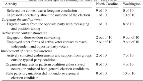
Descriptive summary . . . 65
Conclusions . . . 65
CHAPTER 5: GENERAL DISCUSSION . . . 68
APPENDIX 2.A: CORRELATION MATRIX . . . 71
APPENDIX 2.B: OUTPUT FROM ADDITIONAL MODELS . . . 72
APPENDIX 2.C: DESCRIPTIVE STATISTICS . . . 73
APPENDIX 2.D: MATCHING ANALYSIS . . . 75
APPENDIX 3.A: CODING SCHEME AND INSTRUCTIONS . . . 76
APPENDIX 3.B: BARPLOTS OF PREDICTED OUTCOMES . . . 79
APPENDIX 3.C: MATCHING ANALYSIS . . . 81
APPENDIX 3.D: PREDICTED OUTCOMES, ONE-PARTY CONTESTS . . . 82
LIST OF TABLES
Table
1 Descriptive statistics of contests included in analysis . . . 13
2 Descriptive statistics of spending and vote share data . . . 14
3 Effects on Challenger Vote Share . . . 19
4 Descriptive statistics of candidates included in the analysis . . . 31
5 Descriptive statistics of additional covariates, by contest type . . . 32
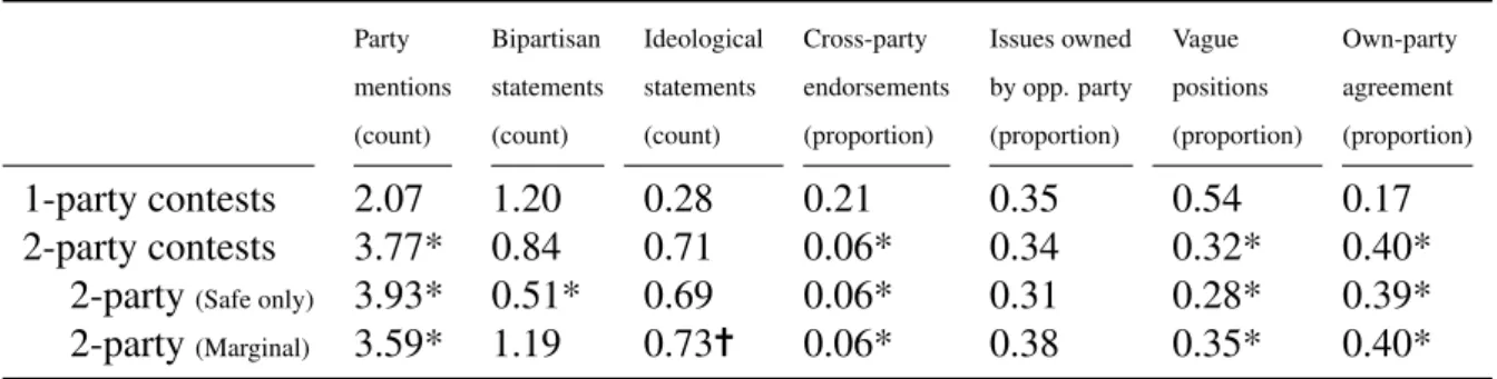
6 Summary statistics of website hand coding, by type of contest . . . 38
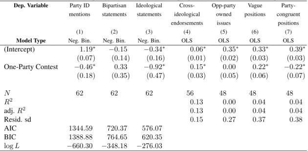
7 Full regression results for all dependent variables . . . 39
8 Effect of one-party contest for each DV, propensity score matched samples . . 40
9 Interview subjects . . . 53
10 Descriptive summary of interview responses . . . 65
11 Matrix of bivariate correlations for variables in analysis . . . 71
12 Effects for challenger vote share, supplemental models . . . 72
13 Descriptive statistics of additional covariates, by contest type . . . 73
14 Descriptive statistics of contests in which groups made independent expenditures . . . 73
LIST OF FIGURES
Figure
1 Distribution of propensity scores for matching analysis . . . 75
2 Count of party ID mentions . . . 79
3 Count of bipartisan statements . . . 79
4 Count of ideological statements . . . 79
5 Proportion of endorsements from groups that typically support opposite party . 79 6 Proportion of issues owned by opposite party . . . 80
7 Proportion of issues with vague or nondirectional positions. . . 80
8 Proportion of issue positions congruent with own party’s position. . . 80
9 Distribution of propensity scores for mentions of party ID, bipartisan statements, and ideological statements as dependent variables . . . 81
10 Distribution of propensity scores for endorsements as the dependent variable . 81 11 Distribution of propensity scores for issues and positions as dependent variables 81 12 Count of party ID mentions . . . 82
13 Count of bipartisan statements . . . 82
14 Count of ideological statements . . . 82
15 Proportion of endorsements from groups that typically support opposite party . 82 16 Proportion of issues owned by opposite party . . . 83
17 Proportion of issues with vague or nondirectional positions. . . 83
CHAPTER 1: INTRODUCTION
In the modern era, partisan elections in the United States are predominately two-stage processes in which candidates must compete in a party primary in the first stage. The winners of each party primary then move on to compete against one other in the general election. The top-two primary changes this process by placing all candidates, regardless of party affiliation, into a single primary in which any voter may choose any candidate. The first and second place finishers in that primary then proceed to a runoff in the general election, even if both
candidates are from the same party. This system is now used in California, Louisiana, and Washington, which are collectively home to one sixth of all Americans.
The top-two primary was implemented by Washington in 2008 and by California in 2012. In both states, advocates hoped that the system would substantively reshape elections and representation in their respective states. In particular, reformers decried the tendency for traditional primaries to nominate polarized candidates that are unrepresentative of their constituencies (Nielson and Visalvanich 2016). At the state legislative level, only about 15 percent of contests nationwide are decided by a margin of 10 percentage points or fewer (Carsey et al. 2008). Since most districts provide a strong electoral advantage to one party, this results in circumstances where one extreme candidate is guaranteed victory by virtue of party labels alone. Advocates of the top-two primary argued that in safe districts, greater choice and competition may be produced when two candidates of the same party advance to the general election. Furthermore, if safe districts offer voters the choice between one extreme and one moderate candidate of the same party in the general election, those safe districts may choose the candidate that best approximates the district median. Over time, reformers hoped that this trend would allow for more accurate representation of mass public, reduce
polarization in government, and mitigate policy gridlock (Pildes 2011).
this research program seeks to understand how same-party general election contests reshape conventional wisdoms about candidate and voter behavior in American politics. More
specifically, I use the context of state legislative elections to evaluate how same-party contests affect the influence of campaign spending, the positions that candidates take when they run for office, and the methods and intensity with which they campaign. In short, I find that the top-two primary produces several important consequences for representative democracy.
History and context
A version of the top-two primary has been used in Louisiana for more than 40 years. In the 1970s, Louisiana was dominated politically by the Democratic party. Governor Edwin Edwards, a Democrat, sought to change the traditional primary process because it was clear that incumbent Democrats (in particular, Governor Edwards) would face their toughest electoral challenges from within their own party. The top-two runoff format was designed to guarantee that Governor Edwards would not be eliminated in the first round of voting. The new top-two primary system was first used in 1975, a year in which he handily won re-election (Mooney 2002). Louisiana’s version of the top-two primary differs from more recent adaptations because any candidate that earns more than 50% in the primary will be elected into office without the need for a runoff election. With this rule, very few contests proceed to a runoff, including fewer than 5% of legislative elections. When runoffs do occur, they are held in late November or early December. Thus, they are characterized by especially low voter turnout. Louisiana has made minor changes to their top-two primary system over the years. For instance, Louisiana did not use the top-two format for congressional elections in 2008 or 2010, and the timing of the primary and runoff has varied.
from party organizations that favor ideologically-extreme candidates1. Voters approved I-872 with 60% of the vote (Galloway 2008) with resistance from major and minor parties alike. The two major parties opposed the reform because same-party contests would prevent them from contesting many seats, while minor parties expected that they would be shut out from virtually all contests in the general election. A challenge found its way to the United States Supreme Court inWashington State Grange v. Washington State Republican Party, but I-872 was upheld as constitutional and the system was implemented in 2008.
In California, Republican State Senator Abel Moldonado, a moderate, is largely credited for his state’s adoption of the top-two primary. For more than a decade leading up to 2009, California’s legislature consistently ranked as the most polarized in the nation (Shor and McCarty 2011). California’s Proposition 13 also requires a two-thirds majority to pass
revenue increases. In 2009, these two factors led to a budget impasse in which Democrats faced resistance to revenue increases during the Great Recession. Democrats needed a single Republican vote to reach the supermajority requirement in the state senate. Senator
Moldenado offered his support, and in return, asked Democrats to place a referendum on the ballot that would offer voters the option of implementing the top-two primary. Moldenado saw the reform as an opportunity to ease polarization and limit future stalemates by creating an environment more conducive to consensus and bipartisanship. If moderates could more easily survive the polarized primary process and get elected to the legislature, he reasoned, then Democrats and Republicans might be better-able to work together. The referendum was approved with 54% of the vote (Caen 2015).
elections, but was rejected by voters in November 2016. Reformers made a second attempt to bring the top-two primary to South Dakota in 2018, this time with a partisan election format, but the effort failed to gather enough signatures to qualify for the ballot.2
Elsewhere, lawmakers have attempted to use legislative pathways to implement the top-two primary. Bills have been introduced in the Arkansas, Illinois, Mississippi, North Carolina, Oregon, and Virginia state legislatures over the past several years. In Congress, a bill that would impose the top-two primary for all congressional candidates was introduced in the U.S. House of Representatives.3 Across a wide range of efforts to enact the system
through both legislative and direct democracy pathways, what remains constant are advocates’ goals of improving the balance of representation, mitigating the effects of polarization, and making elections more competitive.
Overview of dissertation
In the proceeding chapters, three studies investigate how the top-two primary, and the presence of same-party general election contests, affect the competitive electoral environment. These three studies vary in their methods and specific focus, but are bound by a common theme of investigating the implications of the electoral reform for voter and candidate behavior. As reformers pursue adoption of the top-two primary in other states, this research lends insight into the practical implications of those efforts.
In Chapter 2, I find evidence that the presence of a same-party opponent affects the influence of challenger campaign spending in state legislative contests. In two-party contests, voters receive information from party labels and from candidate advertising, which is
facilitated by campaign spending. Combined, this information helps voters make decisions on election day. In the absence of differentiating party labels in one-party contests, the
information provided by candidate spending should matter more. Specifically, I argue that expenditures made by challengers facing same-party opponents should be more effective for increasing vote share than those facing opposite-party opponents. This chapter examines
2South Dakota Secretary of State: https://sdsos.gov
legislative elections in California and Washington, finding that challenger spending in one-party contests increases vote share at more than twice the pace per dollar spent when compared with challengers in two-party contests. Ultimately, results find evidence that the top-two primary changes the competitive electoral environment by helping challengers facing a same-party incumbent to overcome the inherent resource advantages that incumbents enjoy.
In Chapter 3, I investigate the consequences of the top-two primary for candidate rhetoric in one-party contests. Downsian theory (1957) has long informed how scholars think about American two-stage elections, with the conventional wisdom that candidates diverge for the primary and converge in the general election. Recent research, however, finds that
candidates do not adhere to Downsian theory in down-ballot contests. Instead, candidates in U.S. House (Burden 2004) and state legislative (Frendreis et al. 2003) contests remain in their more extreme primary ideological space for the general election. As I will I argue, candidates facing a same-party opponent in the general election should face incentives to self-moderate their positions towards the district median when they can no longer rely on party-based voting to win. In this chapter, I analyze the content of legislative candidates’ campaign websites to find several important differences in the types of rhetoric used by candidates in one-party and two-party contests. First, candidates in one-party contests use more moderate, bipartisan, and vague messaging when compared to those in two-party contests. Furthermore, the party of one’s opponent affects the endorsements that candidates list, the issues that they talk about, and the ways that they talk about those issues.
CHAPTER 2: CAMPAIGN SPENDING AND ELECTORAL COMPETITION4
Political scientists have long sought to understand the many ways in which money shapes electoral outcomes, with much of that attention directed towards better understanding the connection between campaign spending and vote share. Those who have investigated this question at the state legislative level, in particular, have long established that when challengers spend more, they typically will earn a greater percentage of the overall vote in both state legislative primaries (Breaux and Gierzynski 1991; Welch 1976) and general election contests (Gierzynski and Breaux 1991). Others have found that these effects are mediated by several factors. For example, the presence of strong gubernatorial coattails may dampen the effects of spending in state legislative elections (Hogan 2005), while the presence of stricter campaign finance regulations stimulate electoral competition by encouraging quality challenger
emergence (Hamm and Hogan 2008). In this paper, I use the context of the top-two primary to broaden our understanding of how the effectiveness of campaign spending is conditioned by electoral institutions.
States with traditional primaries typically have a process through which the slate of candidates is narrowed to one candidate from each party, if such candidates have filed to run. The top-two primary system differs by placing all candidates for a given position into a single blanket primary. The two candidates with the most votes then proceed to a runoff general election, regardless of their respective party affiliations. This rule allows for contests in which two candidates of the same party may face each other in the general election. The top-two primary, implemented by Washington in 2008 and California in 2012,5provides a venue in which we can further develop our understanding of how electoral rules shape outcomes.
4This chapter previously appeared as an article inElectoral Studies. The original citation is as follows: Sparks, Steven. 2018. “Campaign spending and the top-two primary: How challengers earn more votes per dollar in one-party contests.”Electoral Studies54: 56-65.
Investigating the intended and unintended consequences also offers a practical importance as reformers in other states consider adopting the system.
State legislative elections are typically low-information contests that lack the media attention enjoyed by candidates at the top of the ticket (Kaplan, Goldstein, and Hale 2003). In the absence of information about candidates’ positions, voters often rely on party labels as heuristics to guide preference-consistent choices (see Conover and Feldman 1982; McDermott 1997). When two candidates of the same party face each other in the general election,
however, party labels no longer offer a meaningful signal to facilitate voting decisions. In this paper, I investigate whether the dual absence of media attention and differentiating party cues will raise the effectiveness of challenger campaign spending in state legislative elections. I expect that in one-party contests, challengers will receive a greater increase in vote share per dollar spent when compared with those in two-party contests. This expectation is driven by the importance of campaign spending for establishing name recognition and conveying information to voters, which ultimately earns candidates more votes on Election Day. The present study will test these expectations by analyzing elections data from state legislative contests in California and Washington.6
The top-two primary and electoral behavior
Recent diffusion of the top-two primary beyond Louisiana has inspired some scholarly attention towards investigating its effects. Many have sought to answer whether the top-two primary, as well as similar attempts to open up the primary process, fulfill reformers’ goals of electing more moderate elected officials. Findings are mixed at best. One study finds that California’s experiment with the open blanket primary in the late 1990s indeed produced more victories for moderates in legislative and congressional elections (Gerber 2002). However, an experiment studying the top-two primary find that voters participating in same-party
legislative contests do not have the information necessary to make policy-based distinctions
between their choices, ultimately concluding that moderate candidates fare no better under the system (Ahler et al. 2016). Others find that no moderating effect is observed in the legislators elected under the top-two primary (Kousser et al. 2016) or in California’s previous open blanket primary system in the late 1990s (McGhee et al. 2014).
Some have investigated how the top-two primary affects electoral competition and voting behavior more broadly. Many trends stand out in these early evaluations. First, analysis of California’s legislative elections reveals that zero state legislative incumbents lost their re-election bids from 2002 to 2010, even following the 2000 redistricting (Olson and Ali 2015). However, when the top-two primary was first used in 2012, state legislative
incumbents in California saw a spike in the number of challenges within their own party, with the majority of these challengers emerging in traditionally safe districts (Masket 2012). Ten legislative and congressional incumbents lost their seats in California that year, with six of them losing to same-party opponents. Nine out of the ten intraparty runoffs that year occurred in safe districts. Overall, California was rated as having the most competitive state legislative elections in the country in 2012 (Olson and Ali 2015). It is worth noting that this rise in competition also follows a redistricting cycle and the introduction of a new bipartisan redistricting commission (Grainger 2010). Thus, it is difficult to assess the degree to which increased competition can be attributed to either primary reform or redistricting.
Others have observed a rise in information-seeking among voters participating in state legislative elections in California. When two legislative candidates of the same party faced each other in the general election, leaving voters without a meaningful party cue to distinguish their options, Google searches about those candidates increased by 15% when compared to candidates in two-party contests. No such increase in information-seeking was observed during the first stage of the election (Sinclair and Wray 2015).
The present study seeks to complement and expand upon these findings to further investigate how the top-two primary shapes electoral competitiveness and voter behavior. If challengers are indeed able to earn more votes per dollar spent, such results would reveal one way in which the top-two primary fulfills reformers’ hopes of increased electoral
Voter knowledge in state legislative elections
State legislative elections have long been recognized as low-information contests in which voters possess little or no information with which to make an informed decision on Election Day (Gierzynski and Breaux 1991; Jewell and Olson 1988). Surveys frequently corroborate this claim by revealing a lack of knowledge about state legislators and legislative elections among the majority of voters: a 2006 survey of Utah voters revealed that only 34% could name at least one of their legislators, a 2014 survey of Tennessee voters found that just 44% knew which party controlled their state legislature, and in 2007, only 25% of New Jersey voters were aware that their state legislative elections would be held just two weeks following the date of the survey (Squire and Moncrief 2015).
Despite the lack of voter knowledge regarding state legislators and legislative
elections, most voters are quite adept at using party cues to make meaningful inferences about candidate policy preferences. This facilitates voters’ ability to make preference-consistent vote choices (see Conover and Feldman 1982; McDermott 1997; Tversky and Kahneman 1974). Further, while the specific cause is subject to debate, there is broader consensus that the accuracy and ease with which voters are able to use party cues has improved in recent decades. Whether caused by party sorting (Levendusky 2009; Nivola and Brady 2006), ideological polarization (Abramowitz 2010; Bafumi and Shapiro 2009), or conflict extension (Layman and Carsey 2002), the contemporary party system now presents voters with clearly distinct images of the two major parties. It has thus become easier for inattentive voters to make reasonably accurate approximations of the candidates’ policy preferences based on party labels alone.
votes in down-ballot primaries (Hirano et al. 2015) non-partisan contests (Sheldon and Lovrich 1983), and one-party contests (Ahler et al. 2016), but that the information necessary to do so was less readily available. When such information is provided through candidates’ campaign expenditures, voters should be more likely to use that information when they cannot rely on party labels alone. The top-two primary provides a context in which to test this
expectation.
Campaign spending as a conduit for voter knowledge
One factor contributing to the disparity in voter knowledge in up-ballot versus down-ballot elections is that candidates at the bottom of the ticket receive far less (if any) free media coverage. Anaylsis of the 2002 midterm election reveals that only three percent of campaign stories on local news broadcasts mentioned state legislative contests (Kaplan, Goldstein, and Hale 2003). Therefore, the burden of educating voters about state legislative contests is left to the candidates themselves, and candidate-funded communications are often the primary method through which voters learn about their campaigns (Gierzynski and Breaux 1991). The present research examines how the role of campaign spending as a means for candidates to make themselves known to voters, and therefore increase vote share, is conditioned by the presence of a one-party or two-party contest.
While it is common to hear political observers lament the role of money in politics and the state of the uninformed electorate, higher levels of campaign spending produce
normatively desirable outcomes in low-information contests ranging from judicial elections to U.S. House contests. It is well-established that increased spending in campaigns for state and local offices directly establishes candidate name recognition (Abbe and Herrnson 2003; Krebs 1998). Jacobson (2004) similarly finds that increased campaign spending improves voters’ ability to recall candidates’ names and recognize them in photographs. Campaign spending also improves voter knowledge about candidate policy preferences and raises voter affect towards candidates (Coleman and Manna 2000; Hall and Bonneau 2008). Presumably, however, most candidates’ goal is not to establish name recognition or convey policy
as one such mechanism through which candidates increase their vote share (Kam and
Zechmeister 2013, Kenny and McBurnett 1997; Krebs 1998). At the legislative level, there is evidence that campaign spending increases vote share in general elections (Gierzynski and Breaux 1991), but also in primaries (Breaux and Gierzynski 1991; Welch 1976), where voters tend to be better-informed than the broader electorate.
While these findings demonstrate the importance of challenger spending for electoral competition, the fundraising disparity between incumbents and challengers acts as one barrier to challenger success. Approximately 64% of state legislative races in the U.S. were contested in 2013-2014, but only 18% of contests were considered monetarily competitive.7 In
2013-2014 the better-funded candidate in every legislative contest across 47 states spent an average of $128,477, ranging from approximately $5,000 in Vermont to more than $1,000,000 in California (Holden 2016). The lesser-funded candidate in each contest often fares much worse. Only 2% of legislative contests in Georgia are monetarily competitive, with 5
additional states falling in the single digits. Maine (56%) and Connecticut (51%) are the only states in which at least half of legislative races are monetarily competitive (Holden 2016). Both have public campaign financing systems for legislative candidates.
The importance of this monetary imbalance lies in what it empowers candidates to do with a stark resource advantage. In recent years, state legislative campaigns have undergone a process of “congressionalization,” whereby the activities, outreach tactics, and paid media strategies of legislative candidates increasingly mirror those of congressional campaigns. It is now common for state legislative candidates to hire professional campaign consultants who help them to employ voter outreach strategies such as direct mail, radio, and increasingly, television ads. When challengers are able to fund such efforts, it increases electoral
improving their prospects for success.
Fundraising is not the only barrier to challenger success in legislative elections. As crossover voting has steadily declined, it is also clear that the vast majority of self-proclaimed independents demonstrate voting behavior nearly identical to their partisan counterparts (Keith et al. 1992). Given this trend, the number of persuadable voters in down-ballot contests featuring one Democrat and one Republican is minimal under most circumstances. When this is the case, a challenger might spend as much as they like, but party labels put a ceiling on the number of votes they can earn, creating diminishing returns as spending increases. When both candidates are from the same party, voters must look to other information to drive vote choice. If spending produces higher name recognition and voter knowledge, challengers should observe greater returns on their spending in one-party contests when voters are neither reliant upon, nor bound by, party-based voting.
Summary and expectations
In one-party general election contests, voters lack the ability to use party labels to distinguish their options. Furthermore, down-ballot legislative candidates lack the media attention enjoyed by the top of the ticket. In the dual absence of both media attention and helpful party cues, the information provided by campaign spending should matter more. Thus, I expect that one-party contests enable challengers to earn more votes per dollar spent than challengers in two-party contests.
Data and methods
the websites of the California8and Washington9Secretaries of State to code for challenger vote share. Observations from Louisiana’s top-two primary are excluded from this analysis.10
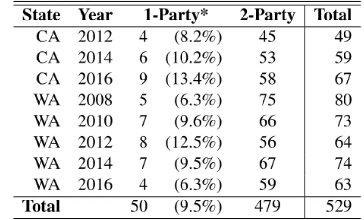
Table 1: Descriptive statistics of contests included in analysis
State Year 1-Party* 2-Party Total
CA 2012 4 (8.2%) 45 49
CA 2014 6 (10.2%) 53 59
CA 2016 9 (13.4%) 58 67
WA 2008 5 (6.3%) 75 80
WA 2010 7 (9.6%) 66 73
WA 2012 8 (12.5%) 56 64
WA 2014 7 (9.5%) 67 74
WA 2016 4 (6.3%) 59 63
Total 50 (9.5%) 479 529
*Parentheses indicate % of total cases that are single-party contests
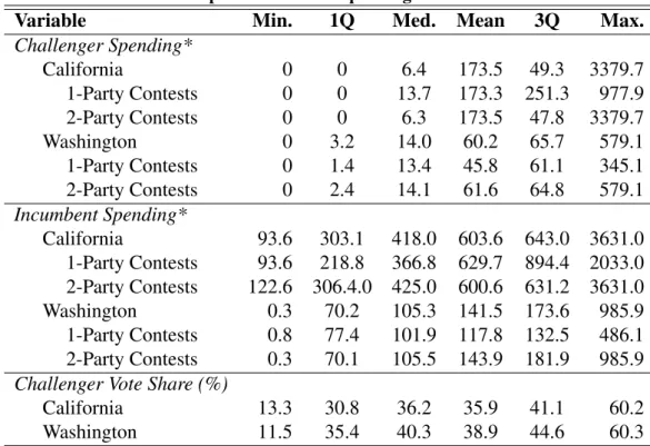
The natural logarithm of the total campaign expenditures for each challenger and each incumbent are included as independent variables for each contest. This transformation follows previous work (Gerber 1998), with the expectation that additional spending should add
positive returns for vote share at all levels of spending, but that the amount of that return per dollar should decrease as spending increases. Spending data are obtained from the
Washington Public Disclosure Commission11and the Cal-Access12website of the California Secretary of State’s Office. Due to the logarithmic transformation, $1 is added to the spending totals of all candidates who made no expenditures. Descriptive statistics of expenditure totals
8http://sos.ca.gov/
9http://sos.wa.gov/
10Louisiana’s top-two primary system differs from its counterparts in that contests only proceed to a runoff if no candidate earns more than 50% of the vote. If there is a majority winner in the primary, there is no second stage election. During the two cycles in which campaign expenditure data are electronically available for Louisiana, 2011 and 2015, only 12 of 288 contests proceeded to a runoff election featuring an incumbent and a challenger. Furthermore, runoff elections in Louisiana typically occur in either late November or early December of odd years, and thus, are marked by extremely low voter turnout. For these reasons, Louisiana contests are excluded from this analysis.
11http://www.pdc.wa.gov
Table 2: Descriptive statistics of spending and vote share data
Variable Min. 1Q Med. Mean 3Q Max.
Challenger Spending*
California 0 0 6.4 173.5 49.3 3379.7
1-Party Contests 0 0 13.7 173.3 251.3 977.9
2-Party Contests 0 0 6.3 173.5 47.8 3379.7
Washington 0 3.2 14.0 60.2 65.7 579.1
1-Party Contests 0 1.4 13.4 45.8 61.1 345.1
2-Party Contests 0 2.4 14.1 61.6 64.8 579.1
Incumbent Spending*
California 93.6 303.1 418.0 603.6 643.0 3631.0
1-Party Contests 93.6 218.8 366.8 629.7 894.4 2033.0 2-Party Contests 122.6 306.4.0 425.0 600.6 631.2 3631.0
Washington 0.3 70.2 105.3 141.5 173.6 985.9
1-Party Contests 0.8 77.4 101.9 117.8 132.5 486.1 2-Party Contests 0.3 70.1 105.5 143.9 181.9 985.9 Challenger Vote Share (%)
California 13.3 30.8 36.2 35.9 41.1 60.2
Washington 11.5 35.4 40.3 38.9 44.6 60.3
*Expenditure totals are presented in thousands of dollars.
are presented in Table 2.13
I also include a dummy variable to indicate whether each contest features two candidates of the same party (one-party contest = 1). The theoretical argument predicts an interactive effect whereby increasing challenger spending generates more vote share per dollar in one-party contests, so I have included two interaction terms: one between the indicator variable for one-party contest and challenger expenditures and a second between one-party contest and incumbent campaign expenditures.
As Gierzynski and Breaux (1991) note, the incumbent’s win margin in the previous election is an important predictor for both candidates’ ability to solicit campaign
contributions, and ultimately, for predicting vote share in election results. Further, past election results are a measure used by state campaign committees when allocating party resources (Gierzynski and Jewell 1989). I follow Gierzynsky and Breaux’s (1991) formula to account for the expected competition in each contest by coding for the incumbent’s win
margin in their previous contest.14
I also include a measure that indicates whether the challenger has previously held elected office, following Jacobson’s (1989) classification of a quality challenger. Challengers with prior elected experience may be more effective candidates due to established donor and volunteer networks, increased name recognition, or because they have established campaign strategies that were successful in previous elections. Jacobson (1989) and others find that candidates that have previously held elective office receive a larger share of the vote and are much more likely to win than their counterparts who have not held elected office. Challengers with prior elected experience may also be more likely to emerge when the incumbent is especially vulnerable. This measure is added to account for any systematic differences in challenger performance that are related to these considerations.
The ideological makeup of each district’s electorate is another important predictor for vote share. I account for district preferences by coding for each district’s ideology score, as developed by Tausonovitch and Warshaw in the American Ideology Project.15 They provide scores for every legislative district for both 2000 and 2010 district boundaries. Contests prior to 2012 are coded with 2000 district scores and contests beginning in 2012 are coded with 2010 scores. However, these scores are produced on a scale centered around 0, with negative scores indicating that a district is more liberal and positive scores indicating that a district is more conservative. I adjust the directional signs of these scores so that they indicate the strength of the challenger’s party, with positive scores indicating greater challenger party strength and negative scores indicating that the challenger’s party is weaker. Put simply, I reverse the sign of the district ideology measure for all contests in which the challenger is a Democrat. To illustrate, a Republican challenger in a conservative district will have a positive score and a Republican challenger in a liberal district will have a negative score. District ideology should have a weaker effect for challenger vote share when both candidates are from
the same party, so an interaction term is included between this variable and one-party contest. Finally, I code each contest with a dummy variable for the challenger’s party
(Democrat = 1), each election year (2008, 2010, 2012, 2014, and 2016) and state (CA and WA), with Washington and 2016 excluded to avoid perfect multicollinearity. Further descriptive statistics of each independent variable are broken down by contest type and presented in Table 13 in Appendix 2.C.
Previous work on campaign spending using ordinary least squares regression finds that incumbents will earn the highest percentage of the vote when they spend the least, while challengers will see their vote share rise with increased spending (for examples, see Cassie and Breaux 1998; Gierzynski and Breaux 1991). Such predictions appear logically
inconsistent, as this suggests that incumbents facing a strong, well-funded challenger will be most likely to win if they spend no money at all. However, as we know, these findings make more sense when we account for the fact that safe incumbents need not spend great sums of money to win handily, while those facing electoral trouble may spend much more and earn a much smaller margin of the overall vote. Many have noted that accurately predicting the effects of incumbent campaign expenditures for incumbent vote share is difficult because it is endogenously shaped by expectations of success (see Jacobson 1980; Green and Krasno 1988). As Jacobson (2006) notes, the use of ordinary least squares regression in such studies is found to bias estimates upward for challenger spending and bias estimates downward for incumbent spending.16 The present study focuses on how challenger spending in one-party contests compares with challenger spending in two-party contests, not on comparisons
between challenger and incumbent spending. Thus, the degree of bias, if any, will be the same across the two contexts, unlike comparisons between incumbent and challenger spending. Therefore, concerns about bias do not apply and the use of OLS is appropriate in this context.
In sum, the theoretical argument motivates the following model using ordinary least squares regression:
yi =β0+β1X1 +β2X2+β3X3+β4(X1∗X3) +β5(X2∗X3) +β6X4+β7X5
+β8(X5∗X3) +β9X6+β10X7+β11X8+β12X9+β13X10+β14X11+β15X12+i
where yi=Challenger Vote Share
X1=Natural Log of Challenger Spending X2=Natural Log of Incumbent Spending
X3=One Party Contest
X4=Incumbent Previous Win Margin X5=District Ideology
X6=Challenger Party (1 = Democrat) X7=Quality Challenger (1 = Yes)
X8=2008 X9=2010 X10=2012
X11=2014 X12=California
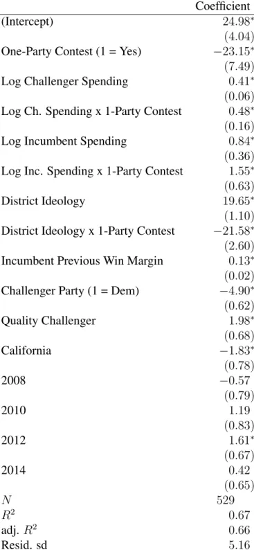
Results
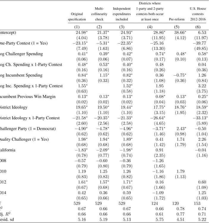
Model estimates are presented in Table 3. I expected that increasing challenger campaign spending would generate greater vote share per dollar spent in one-party contests than in two party contests. Findings provide support for this prediction, with the interaction term between log challenger spending and 1-party contest positive and significant at the 0.05 level. Challengers in one-party contests, on average, earn more than twice as many votes per unit increase in spending than challengers in two-party contests. Interpreting the coefficients of the log transformed variables, each 100% increase in challenger spending translates to an average .41 percentage point increase in challenger vote share in two-party contests.17
Meanwhile, a 100% increase in challenger spending produces an average .89 percentage point
17This interpretation of the coefficient follows Gujarati (2003, p. 183) in which the coefficient for a log-transformed independent variable in OLS regression is interpreted as a 1% change inX corresponding with a
increase for challenger vote share in one-party contests.18. In practical terms, suppose Challenger A is running in a one-party contest and Challenger B is running in a two-party contest. Now, suppose each candidate spends a total of $13,000, which is roughly the median level of expenditures across contest type. All else equal, if each candidate doubled their expenditures from $13,000 to $26,000, Candidate A could expect to increase her vote share by .89 percentage points while Candidate B could expect to incease her vote share by .41 percentage points. Doubling expenditures again to $52,000 would earn Candidate A yet another .89 percentage points and earn Candidate B an additional .41 percentage points.19
Given the dispersion of the data for spending totals, I estimated the effect of influential cases for these results using Cook’s Distance. With all influential cases removed, challengers still earn more than twice as many votes per dollar spent.20
I also investigate whether characteristics unique to districts where one-party contests occur are driving the results through selection bias. For this test, I re-run the analysis by only including observations from districts that saw at least one one-party contest and at least one two-party contest occur during the included years. With all other observations excluded, this sample includes 38 of the 50 one-party contests and 86 two-party contests, across 25 districts. The interaction term between challenger spending and one-party contest is significant at the
18Here, the coefficient for challenger spending in one-party contests is calculated, using the model outlined on page 11, asβ1+β4X3= 0.41+0.48(1) = 0.89.
19To investigate possible effects of multicollinearity, I perform the following checks. First, I report bivariate correlation coefficients among the independent variables in a correlation matrix, found in Appendix 2.A. A possible concern is that challenger and incumbent spending might be highly correlated because closely-contested contests and those in expensive media markets are likely to see increased spending by both candidates. The correlation coefficient between incumbent and challenger spending is 0.17. Second, I calculate the variance inflation factors (VIFs) for each coefficient. Two variables have VIFs larger than 10:1-Party Contestand the interaction term1-Party x Log Incumbent Spending. If this interaction term is omitted from the model, the VIF for1-Partydrops to 4.44. Regression output for the model with this interaction term omitted is reported in column 2 of Table 12 in Appendix 2.B. In this model, the coefficient for the variable of interest, the interaction term1-Party x Log Challenger Spending, is still significant. The substantive finding remains: challengers in one-party contests earn more than twice as many votes per dollar spent than those in two-one-party contests.
20There were 37 observations withD
Table 3:Effects on Challenger Vote Share
Coefficient
(Intercept) 24.98∗
(4.04)
One-Party Contest (1 = Yes) −23.15∗ (7.49)
Log Challenger Spending 0.41∗
(0.06)
Log Ch. Spending x 1-Party Contest 0.48∗ (0.16)
Log Incumbent Spending 0.84∗
(0.36)
Log Inc. Spending x 1-Party Contest 1.55∗ (0.63)
District Ideology 19.65∗
(1.10)
District Ideology x 1-Party Contest −21.58∗ (2.60)
Incumbent Previous Win Margin 0.13∗ (0.02)
Challenger Party (1 = Dem) −4.90∗ (0.62)
Quality Challenger 1.98∗
(0.68)
California −1.83∗
(0.78)
2008 −0.57
(0.79)
2010 1.19
(0.83)
2012 1.61∗
(0.67)
2014 0.42
(0.65)
N 529
R2 0.67
adj. R2 0.66
Resid. sd 5.16
Standard errors in parentheses
.1 level with this smaller sample. Results are consistent with the broader analysis, finding that challengers in one-party contests maintain a strong advantage by earning approximately 60% more votes per dollar spent than those running in two-party contests. Results are presented in column 4 of Table 12.
To investigate the possibility that results are confounded by systematic variation among the independent variables between one-party and two-party contests, I use propensity score matching to estimate the average treatment effect of running in a one-party contest. Using theMatchIt21package in R, I employ nearest-neighbor matching with a caliper of .2 standard deviations. This method matched 46 of the 50 one-party contests to 46 two-party contests across a series of covariates.22 Figure 1 in Appendix 2.D presents the distribution of propensity scores for matched and unmatched treatment and control groups. I run OLS regression with these 92 matched observations, with challenger vote share as the dependent variable and one-party contest as the independent variable. All else equal, the average
treatment effect of running in a one-party contest provides a 5.40 percentage point increase in challenger vote share within the matched sample, significant at the .05 level. Results are presented in Table 17 in Appendix 2.D.
Column 5 in Table 12 presents results for observations that occurred prior to the adoption of the top-two primary. This model includes only contests from 2006 in Washington and 2010 in California, the cycles that immediately preceded implementation of the reform in each state.
Investigating the role of independent expenditures
An alternative explanation for these findings is unrelated to the role of voter
information altogether. Rather, one possibility is that parties and interest groups direct their independent expenditures towards two-party races because they believe that their finite resources are best spent contesting seats where party control is in question. Given the
21Ho, Daniel, Kosuke Imai, Gary King, and Elizabeth Stuart. 2011. “MatchIt: Nonparametric Preprocessing for Parametric Causal Inference.”Journal of Statistical Software, 42: 1-28. http://www.jstatsoft.org/v42/i08/
diminishing returns of campaign spending for vote share as totals increase (Gerber 1998), the disproportionate direction of independent expenditures into two-party contests may explain why challengers in one-party contests see a greater return for each dollar spent. To determine the viability of this explanation, I coded each contest with the amount of independent
expenditures made on behalf of both the incumbent and the challenger using data available online from the Washington Public Disclosure Commission23and Cal-Access24websites. Independent expenditures that are listed as opposing the incumbent are included with the challenger’s totals, while expenditures classified as opposing the challenger are included with the incumbent’s totals. Descriptive statistics of independent expediture data are presented in Tables 7 and 8 in Appendix 2.C.
To best capture the mechanism of diminishing returns per dollar spent, I combine candidate spending and independent expenditures on the candidate’s behalf into a single total and then logarithmically transform that total. In Appendix 2.B, column 3 in Table 12 presents OLS regression output when independent expenditures are included with candidate spending. In this model, the coefficients for challenger spending and the interaction term between challenger spending and one-party contests both remain significant at the .05 level. Here, a challenger in a two-party contest can expect to receive an average 0.42 percentage point increase in vote share for every 100% increase in spending, while a challenger in a one-party contest can expect to earn a .82 percentage point increase for every 100% increase in
spending. When independent expenditures are included, challengers in one-party contests can still expect to earn nearly twice as many votes per dollar spent.
Effects for spending in higher-information campaign environments
To further test the theoretical argument, I perform the same analysis with U.S. House candidates. Congressional elections are likely to enjoy greater media attention and general voter awareness than state legislative elections. When candidates are running in
higher-information environments, the benefit of spending in the absence of differentiating
party labels should be weaker. Thus, the observed effect of candidates in one-party legislative contests earning twice as many votes per dollar should be smaller at the congressional level.
For this analysis, I include all U.S. House elections in California and Washington from 2012-2016.25 There were a total of 153 contests with both an incumbent and challenger on the general election ballot during this period. Of those, 16 were one-party contests and 137 were two-party contests.26 Data were collected in the same manner as with state legislative seats, with two modifications. First, spending data were collected from the Federal Elections Commission rather than the respective secretaries of state. Second, congressional district-level ideology scores were used from Tausonovitch and Warshaw’s American Ideology Project27.
Regression results for congressional contests are reported in column 6 of Table 12. The coefficient for challenger spending is positive and significant, but the interaction term between challenger spending and one-party contests is not statistically significant.
Challengers in one-party congressional contests enjoy no advantage in the number of votes they earn per dollar spent when compared to challengers in two-party congressional contests.
Discussion
Many have replicated the finding that challengers will, on average, earn more votes when their campaigns spend more money. In the present study, I have expanded our
understanding of this effect by showing that electoral rules are likely to dictate the degree to which challengers are able to translate their dollars into votes. In fact, a challenger running in a single-party contest can expect to typically increase their vote share at double the pace per dollar spent when compared to challengers in two-party contests. Ultimately, the present findings provide evidence that the effects of campaign money are muted when party labels provide meaningful information to voters. However, in the absence of differentiating party cues to guide vote choice, the information provided by campaign expenditures has a much larger effect for increasing challenger vote share and overcoming the advantages inherent to
25There were no one-party congressional contests in Washington in 2008 or 2010.
26Descriptive statistics of these data are reported in Table 16 in Appendix 2.C.
incumbency. Put simply, challengers in one-party contests are able to get a bigger bang for their buck, which better equips them to overcome the inherent advantages of both funding and name recognition enjoyed by incumbents.
When reformers implemented the top-two primary, one intended goal was to increase electoral competition when two candidates of the same party proceed to a runoff in the general election in traditionally safe districts (Pildes 2011). While little research to date measures whether the top-two primary has increased competition, the present study fills this gap by offering evidence that it does indeed provide opportunities for greater competitiveness in single-party contests. Advocates of the top-two primary, as well as those who lament the lack of electoral competition in legislative elections, may be encouraged by these findings.
The results of this study also suggest a reconceptualization of what constitutes a “safe” district. When single-party general election contests occur in top-two primary states, it is most often in districts that are among the safest for one party or the other. In such districts,
potential candidates that have ambitions for elected office may be dissuaded from running when an incumbent chooses to seek re-election, especially if they are from the same party. However, quality candidate entry is one of the most important factors that affects whether incumbents retain their seats (Jacobson 1989; Hetherington et al 2003). Nationwide, nearly half of legislative seats were uncontested in 2016 (Greenblatt 2016), with a lack of
CHAPTER 3: CANDIDATE RHETORIC AND POLARIZATION28
In many ways, primary elections advance the interests of extreme party factions. In part, primary candidates are likely to adopt extreme views to cater to passionate partisan voters (Brady et al. 2007), who are likely to prefer extreme candidates that align with the party base (Nielson and Visalvanich 2016). In recent years, moderate incumbents in both parties have increasingly been eliminated in primaries by more extreme challengers. Although Downs (1957) theorized that rational candidates should converge to the median voter in the general election, very few legislative and congressional districts are competitive in the general election today. As a result, much evidence finds that most candidates do not converge in down-ballot contests (Burden 2004; Frendreis et al. 2003).
Under the top-two primary, all candidates for a given office run against each other in a single blanket primary, regardless of party. Whichever two candidates receive the most votes will then proceed to a runoff in the general election. Many have decried that runoff elections between two candidates of the same party are the ultimate advancement of extreme partisan interests (Feinstein 2016; Greenhut 2016). In this paper, I investigate candidate rhetoric under the top-two primary and find evidence to the contrary. As I will argue, new electoral rules encourage candidates to appeal to a broader range of voters in one-party contests.
For several years leading up to 2009, California was home to the most polarized state legislature in the nation (Shor and McCarty 2011). During the Great Recession, this
polarization contributed to a budget stalemate in which Democrats needed one Republican vote to reach the two-thirds supermajority threshold required for revenue increases. State Senator Abel Moldenado, a moderate Republican, offered to support the budget if Democrats supported a voter referendum that, if passed, would implement the top-two primary.
Moldenado saw the reform as an opportunity to prevent future stalemates by creating an environment conducive to consensus and bipartisanship. If moderates could more easily survive the polarized primary process, he reasoned, the ideological distance between the median chamber Democrat and Republican might narrow (Caen 2015).
Prior examination of legislative elections under the top-two primary, however, finds that voters do not select the more moderate of two same-party candidates because they lack the information to make preference-consistent choices (Ahler et al. 2016). This is
unsurprising, given that legislative elections are low-information contests in which voters are notoriously uninformed (Gierzynski and Breaux 1991; Squire and Moncrief 2015). I
investigate another pathway through which Moldenado’s aspirations to invoke moderation may be realized. Top-two primaries change the mix of opponents that candidates face, thus altering the electorate to which they must respond. When candidates face a same-party general election opponent, they can no longer rely on party-based voting to win. In such contests, every voter and constituency may be persuadable. Thus, candidates in one-party contests should face pressures to broaden the set of voters to whom they appeal, even in districts that strongly favor one party. Much research supports this theory, showing that the presence of electoral competition leads candidates to adjust their campaign strategies (Banda and Carsey 2015; Fowler 2005) and encourages responsiveness to the median voter
(Ansolabehere et al. 2001; Hayes et al. 2002).
To test this expectation, I evaluate the rhetoric found on the campaign websites of state legislative candidates in California and Washington during the 2016 election. I compare the rhetoric used by candidates facing same-party and opposite-party opponents, finding strong evidence that candidates in same-party contests use more bipartisan, moderate, and vague language than those in two-party contests. Furthermore, the presence of a same-party contest conditions the issues that candidates talk about, how they talk about those issues, and
encourages more endorsements from groups that typically support the opposite party.
Voter behavior and the top-two primary
expectations of invoking moderation in one-party contests. First, an experiment during the 2012 general election in California found that moderate candidates in one-party contests fared no better than their more liberal or conservative opponents. Even when voters preferred the more centrist option, the study found that voters lacked the information necessary to distinguish between two same-party options (Ahler et al. 2016). Second, when both candidates are from the same party, voters from the opposite party are much more likely to abstain from voting in that contest rather than supporting the ideologically-proximate choice (Fisk 2017; Nagler 2015). Finally, even when voters are informed, evidence suggests that many moderates vote based on factors unrelated to ideology or issue preferences altogether (Adams et al. 2017).
Collectively, these findings cast doubt on the idea that voters will invoke moderation in state legislative elections under the top-two primary. This should be no surprise, given that legislative elections are low-information contests in which voters typically have very little knowledge (Gierzynski and Breaux 1991; Squire and Moncrief 2015). Attention to legislative elections makes up only three percent of campaign-related local news coverage (Kaplan, Goldstein, and Hale 2003). In one-party contests under the top-two primary, the combined absence of media attention and helpful party cues means that the information conveyed by campaign spending has a greater influence on vote choice. Challengers running against a same-party incumbent in the general election earn twice as many votes per dollar than those running against an opposite-party incumbent (Sparks 2018).
While prior research finds no evidence that voters impose moderation in one-party contests, there is reason to expect that new electoral conditions may encourage any number of changes in candidate behavior. One possibility is that candidates will respond as critics expected: by becoming even more ideologically extreme. Same-party contests
of their party and allied groups will be crucial to success. This incentive may likewise encourage candidates to exclusively target base voters. These potential pressures, however, should be outweighed by incentives for candidates to broaden their appeal beyond the party base. I argue that the pressures candidates face in one-party general election contests are distinct from those that they face in primaries and in most two-party general elections. One-party contests produce electoral uncertainty and broaden the constituency to whom candidates are accountable. Combined, these pressures should encourage candidates to self-impose moderation when facing a same-party opponent.
Candidate behavior and the top-two primary
Interviews with California state legislators lend anecdotal insight by showing how the top-two primary liberates lawmakers from the confines of strict party discipline. Republican State Senator Anthony Cannella explains that the top-two system enabled him to co-sponsor bipartisan legislation permitting undocumented immigrants to obtain drivers licenses, an issue he previously avoided. His Republican colleagues likewise perceived that their re-election constituencies now expand beyond the extreme wing of primary voters (Olson and Ali 2015). This example illustrates how the top-two primary may reshape candidate and legislator
behavior as electoral incentives change. The perceived risk of backlash from party base voters when candidates demonstrate bipartisanship is diminished with this change in electoral rules.
Conventional wisdom has long held that candidates maximize their electoral prospects by making calculated decisions about how they present themselves to voters. Mayhew
Much work supports the notion that candidates do diverge to the ideological extremes for the primary election (Brady et al. 2007; Fiorina 1974; Polsby 1980). Some find evidence that candidates do converge back towards the median for general election in U.S. Senate (Wright and Berkman 1986), gubernatorial (Carsey 2000), and presidential elections (Acree et al. 2013). Others find that Downsian theory does not hold up in U.S. House and legislative contests, with candidates in these contexts instead largely remaining at the ideological extremes for the general election (Aldrich and Coleman Battista 2002; Burden 2004; Frendreis et al. 2003).
A likely explanation for this difference is that most U.S. House and legislative elections are not competitive, thus, most candidates lack incentive to court the median voter. Nationwide, only 30% of legislative seats are decided by fewer than 20 percentage points, with only 15% of seats decided by fewer than 10 percentage points (Carsey et al. 2008). From 2003 to 2014, one-third of all legislative seats were uncontested. During the 2013-2014 cycle, more than half of seats were uncontested in 13 states. This lack of competitiveness is
intensified by a stark imbalance in candidate fundraising, with only 18% of legislative contests being monetarily competitive29in 2013-2014 (Holden 2016). This resource imbalance prevents both candidates enjoying the same quality of staff support, advertising, and voter outreach strategies, thus tipping the scales even more in favor of one candidate.
Furthermore, very few voters are persuadable. Although 40% of voters identify as independents, 85% of independents demonstrate voting behavior indistinguishable from their partisan counterparts (Smith 2016). This effect is more pronounced in low-information contests such as legislative elections, where voters are most likely to rely on party labels to guide their vote choices (Schaffner and Streb 2002). Combined with the lopsided nature of most legislative contests, this means the outcome is often a foregone conclusion. In most races, candidates are practically guaranteed to win or lose by virtue of party labels alone.
When both candidates are from the same party in the general election, however, they can no longer rely on party-based voting to win. If candidates cannot reliably predict for
whom Republicans and Democrats will vote, they should respond accordingly. I argue that the presence of one-party general election contests should create uncertainty and competitiveness that is not present in most two-party contests at the legislative level. This should incentivize candidates to self-moderate their rhetoric in an effort to appeal to as many voters as possible.
The proposition that candidates should moderate their behavior against a same-party opponent relies on two premises: first, that candidates behave as though issues matter to voters, and second, that candidates adjust their campaign strategies based on contextual factors. There is much evidence that candidates behave as though voters are paying attention and that candidates are responsive to those voters when electoral pressure exists.
Ansolabehere et al. (2001) find that while national and state party pressures influence candidate position-taking, that district-level voter preferences likewise matter. King (1997) demonstrates how signs of vulnerability lead candidates to engage in risk-averse behavior. Fowler (2005) shows how candidates calibrate their campaign platforms in response to the outcome of the previous election. Lawmakers also adapt legislative efforts in response to changes in the demographic makeup of their districts after redistricting (Hayes, Hibbing, and Sulkin 2010; Overby and Cosgrove 1996). Even if most voters are largely inattentive, many credit interest groups, challengers, and the media for monitoring behavior and alerting voters when candidates stray from the district median (Canes-Wrone et al. 2002; Carsey 2000).
Expectations
If candidates behave as though issues matter to voters, are responsive when
incentivized, and adjust strategy based on context, then the top-two primary should encourage candidates in same-party contests to broaden their appeal. Imagine a district that reliably votes 70% Democratic and 30% Republican. Under traditional primary rules, neither
candidate has incentive to temper their message when the outcome of the general election is a foregone conclusion. Now, suppose that two Democrats face each other in the general election in that same district, and suppose that they expect to split the Democratic vote. The 30% of voters who were once irrelevant may now theoretically swing the election. To be clear, the argument is not that Democratic candidates in a 70/30 district will become conservatives or even centrists. Rather, I expect that they should adjust at least somewhat towards a closer approximation of the district median than they would under traditional primary rules. In doing so, they should use more moderate and bipartisan rhetoric in their campaign messaging.
If correct, there are several behaviors we should expect to observe. First, candidates in one-party contests seeking to broaden the range of voters to whom they appeal should make fewer mentions of their party identity, fewer clear statements about the ideological direction of their views, and more statements about the importance of bipartisanship.
Second, candidates in one-party contests should be more likely to advertise
endorsements from ideological groups or partisan figures that typically support the opposite party. Endorsements send signals about a candidate’s policy preferences, from which voters form evaluations about that candidate (McDermott 2006). If candidates in one-party contests seek to broaden their appeal, a larger proportion of their endorsements should be from beyond their traditional coalitions.
positions in agreement with their own party.
Data
To evaluate the degree to which candidates fulfill these expectations, I analyze the content of campaign websites for state legislative candidates in California and Washington30 during the 2016 election. I select websites as the best data source using the criteria proposed by Druckman et al. (2009). First, websites are unfiltered communications direct from each campaign, whereas media coverage or interest group ratings are colored by the lens of the journalist or group. Second, websites represent a comprehensive view of candidates’ positions, whereas voter guide statements are often restricted to as few as 100 words (Druckman et al. 2009).
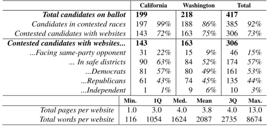
Table 4:Descriptive statistics of candidates included in the analysis
California Washington Total
Total candidates on ballot 199 218 417
Candidates in contested races 197 99% 188 86% 385 92%
Contested candidates with websites 143 72% 163 75% 306 73%
Contested candidates with websites... 143 163 306
...Facing same-party opponent 31 22% 15 9% 46 15%
... In safe districts 90 63% 84 52% 174 57%
...Democrats 81 57% 80 49% 161 53%
...Republicans 61 43% 74 45% 135 44%
...Independent 1 1% 9 6% 10 3%
Min. 1Q Med. Mean 3Q Max.
Total pages per website 1.0 3.0 4.0 3.8 4.0 13.0
Total words per website 116 1054 1624 2087 2735 8674
I use the California and Washington Secretary of State websites to identify the
universe of contested legislative candidates. Those running in uncontested races are excluded because they have neither electoral pressure nor motivation to be concerned with how they position themselves. I then search for the campaign website of each contested candidate. Several methods are employed: Google searches, lists from state party websites, links listed in voter guide statements, links from social media pages, and local print media coverage.
question investigates the behavior of partisans under varying electoral conditions. This provides a total sample of 296 websites.
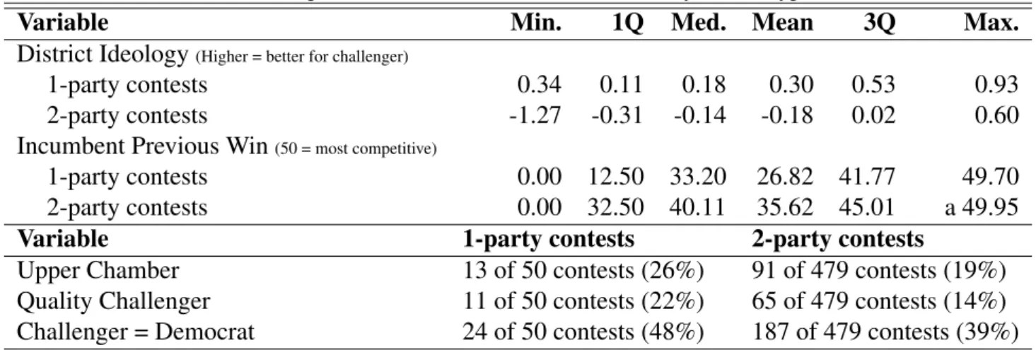
Table 5:Descriptive statistics of additional covariates, by contest type
Variable Min. 1Q Med. Mean 3Q Max.
District Ideology(Lower = favorable for candidate)
1-party contests -1.22 -0.58 -0.38 -0.44 -0.11 0.00
2-party contests -1.27 -0.22 -0.02 -0.02 0.16 1.15
Incumbent Previous Win(50 = most competitive)
1-party contests 0.00 20.05 30.85 27.98 40.20 49.50
2-party contests 0.00 32.64 40.32 36.45 44.33 49.93
Variable 1-party contests 2-party contests
Upper Chamber 11 of 46 candidates (24%) 45 of 250 candidates (18%) Democrat 13 of 46 candidates (28%) 127 of 250 candidates (51%) Challenger 10 of 46 candidates (22%) 91 of 250 candidates (36%) Open seat 25 of 46 candidates (54%) 50 of 250 candidates (20%)
Margin btw. Clinton/Trump in district Min. Mean Med. Max.
All candidates 0% 31% 29% 83%
Candidates in 1-party contests 8% 41% 43% 83%
Snapshots of each website were saved during the two weeks prior to the November 8, 2016 election. When available, data include the ‘Home,’ ‘About,’ ‘Issues,’ and
‘Endorsements’ pages from each site. If candidates had multiple pages for separate issues, each ‘Issues’ subpage is included. No additional pages are included in the analysis. Descriptive statistics of the candidates and websites included in the data are presented in Table 4. Descriptive statistics comparing candidates in one-party and two-party contests across several covariates are presented in Table 5.
Methods
Coding website content
I code the content each website on several measures to test the theoretical expectation that candidates in one-party contests will have websites that use more moderate and bipartisan rhetoric than those in two-party contests. The coded count or proportion for each of the following variables is cumulative across all captured pages of the website. These counts and proportions then serve as dependent variables for a series of seven regressions. To validate coding decisions made by the author, a research assistant coded a random sample of 47 of the 296 websites.31