Admission Control and Routing in Multi-priority Systems
by Feng Chen
A dissertation submitted to the faculty of the University of North Carolina at Chapel Hill in partial fulfillment of the requirements for the degree of Doctor of Philosophy in the Department of Statistics and Operations Research.
Chapel Hill 2006
Approved by
Advisor: Professor Vidyadhar G. Kulkarni Reader: Professor Amarjit Budhiraja Reader: Professor Chuanshu Ji
c
2006
Feng Chen
ABSTRACT
Feng Chen: ADMISSION CONTROL AND ROUTING IN MULTI-PRIORITY SYSTEMS
(Under the direction of Professor Vidyadhar G. Kulkarni)
We consider a manufacturer that offers two types of prioritized warranties for its product. Type 1 warranty guarantees a shorter turnaround time than type 2 warranty. Hence items covered by type 1 warranty receive higher priority in repair service. When an item under warranty fails, the manufacturer sends it to one of several repair vendors for repair, who are under contracts to provide repair service for the manufacturer. The manufacturer pays each vendor a fixed fee per repair assignment. While an item is at the vendor under or awaiting repair, a linear holding cost is incurred by the vendor and a linear good-will cost is incurred by the manufacturer.
policy, while it can accept either more or fewer low-priority customers than either of the other two optimal policies.
ACKNOWLEDGMENTS
I would like to express my deepest gratitude to my advisor, Professor Vidyadhar G. Kulkarni, for introducing me to the stochastic modeling area and for his priceless encouragement and guidance throughout the research. I am extremely grateful for his wise advice on my career path, which made the completion of the dissertation not only possible but also a truly enjoyable and rewarding experience.
CONTENTS
LIST OF TABLES . . . viii
LIST OF FIGURES . . . ix
LIST OF SYMBOLS . . . x
1 Introduction 1 1.1 Overview . . . 1
1.2 Literature Review . . . 3
1.2.1 Admission Control . . . 4
1.2.2 Warranty Repair Routing . . . 5
2 Admission Control: Value Iteration Approach 9 2.1 Problem Description . . . 9
2.2 Individual Optimization . . . 10
2.3 Class Optimization . . . 14
2.4 Social Optimization . . . 24
2.5 A Special Case for Social Optimization . . . 29
2.6 Comparison and Numerical Results . . . 32
3 Admission Control: Sample Path Approach 46 3.1 Problem Description . . . 46
3.2 Individual Optimization . . . 47
3.3 Social Optimization . . . 47
3.4.1 Optimal Policies for Class 1 . . . 59
3.4.2 Optimal Policies for Class 2 . . . 62
3.5 Numerical Comparison . . . 63
4 Dynamic Routing 68 4.1 Problem Description . . . 68
4.2 Heuristics . . . 69
4.2.1 Optimal State-Independent Policy (OSI) . . . 69
4.2.2 Generalized Join the Shortest Queue Policy (GJSQ) . . . 73
4.3 Simulation Study . . . 86
5 Conclusions and Future Work 95 5.1 Conclusions . . . 95
5.2 Future Work . . . 96
Appendix 98
LIST OF TABLES
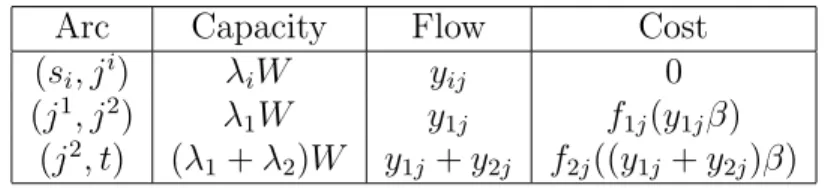
Table 4.1 Arc properties for the network representation of (4.7) . . . 72
Table 4.2 Cost reduction of GJSQ over JSQ . . . 91
Table 4.3 Cost reduction of GJSQ over OSI . . . 92
Table 4.4 Cost reduction of GJSQ over T . . . 92
Table 1 Simulation parameters (Trials 1-25) . . . 99
Table 2 Simulation parameters (Trials 26-50) . . . 100
Table 3 Simulation parameters (Trials 51-75) . . . 101
Table 4 Simulation parameters (Trials 76-100) . . . 102
Table 5 Simulation parameters (Trials 101-125) . . . 103
Table 6 Simulation parameters (Trials 126-150) . . . 104
Table 7 Simulation parameters (Trials 151-175) . . . 105
LIST OF FIGURES
Figure 2.1 Class 1 switching curves . . . 43
Figure 2.2 Class 2 switching curves: case 1 . . . 43
Figure 2.3 Class 2 switching curves: case 2 . . . 44
Figure 2.4 Class 2 switching curves: case 3 . . . 44
Figure 2.5 Class 2 switching curves: case 4 . . . 45
Figure 2.6 Class 2 switching curves: case 5 . . . 45
Figure 3.1 Class optimization for class 1: v against i . . . 65
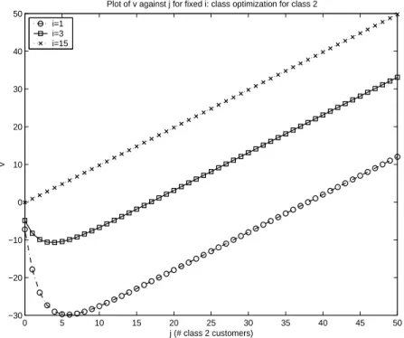
Figure 3.2 Class optimization for class 2: v against j for fixed i . . . 65
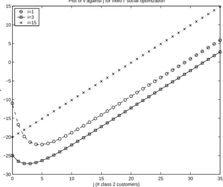
Figure 3.3 Social optimization: v againsti for fixed j . . . 66
Figure 3.4 Social optimization: v againstj for fixed i . . . 66
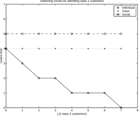
Figure 3.5 Class 1 switching curves . . . 67
Figure 3.6 Class 2 switching curves . . . 67
Figure 4.1 Network model of two-priority problem . . . 72
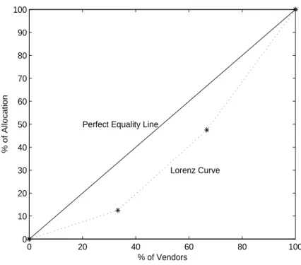
Figure 4.2 Lorenz curve and perfect equality line . . . 89
Figure 4.3 Cost reduction of GJSQ over JSQ . . . 93
Figure 4.4 Cost reduction of GJSQ over OSI . . . 93
LIST OF SYMBOLS
α discount rate
β failure rate of each item
B1 busy period for serving type 1 items initiated by a single type 1 item
B2 busy period for serving both types of items initiated by a single type
2 item
C11 expected holding cost incurred by the type 1 items during B1
C12 expected holding cost incurred by the type 1 items during S2
G Gini coefficient of initial state-independent allocation hi holding cost rate of each class icustomer
H1(x1, x2) expected total holding cost incurred by the system starting from
initial state (x1, x2) until time T1(x1)
H2(x1, x2) expected total holding cost incurred by the system from timeT1(x1)
until time T(x1, x2)
H(x1, x2) expected total holding cost incurred by the system starting from
initial state (x1, x2) until time T(x1, x2)
I1j(x1j, x2j) class 1 index at vendor j in state (x1j, x2j) I2j(x1j, x2j) class 2 index at vendor j in state (x1j, x2j)
LC
1 threshold for accepting class 1 customers under class optimization
LI
1 threshold for accepting class 1 customers under individual
optimiza-tion LS
1(j) threshold for accepting class 1 customers under social optimization
when there are j class 2 customers in the system LC
2(i) threshold for accepting class 2 customers under class optimization
when there are i class 1 customers in the system LI
2(i) threshold for accepting class 2 customers under individual
optimiza-tion when there are i class 1 customers in the system LS
2(i) threshold for accepting class 2 customers under social optimization
λi arrival rate of class icustomers Λ uniform rate
µ repair service rate φk λkW β
φi(α) E(e−αT|X(0) =i)
pki Bernoulli splitting probability of assigning a type k item to vendori p∗
ki optimal Bernoulli splitting probability of assigning a type k item to vendor i
pk (pk1, pk2,· · ·, pkV)
p∗k (p∗k1, p∗k2,· · ·, p∗kV)
P P(λ) Poisson process with rate λ
ri reward for accepting a class i customer
S2 the service completion time of a type 2 item accounting for
interrup-tions from type 1 items. Thus if a type 2 item starts service at time 0, it will complete service at time S2
τ1(x1) E(T1(x1))
τ(x1, x2) E(T(x1, x2))
T min{t≥0 :X(t) = 0}
T1(x1) min{t≥0 :X1(t) = 0|X1(0) =x1}
T(x1, x2) min{t≥0 :X1(t) = 0, X2(t) = 0|X1(0) =x1, X2(0) =x2}
v(i, j) minimum expected total discounted cost starting from state (i, j) vn(i, j) nth-step value function generated by value iteration algorithm
V set of functions defined on {(i, j) : i ≥ 0, j ≥ 0} that satisfy mono-tonicity in i and j, supermodularity, and diagonal dominance in j ¯
V total number of repair vendors W warranty length
bxc largest integer less than or equal to x
X(t) number of customer in an M/M/1/k queue at timet Xk(t) number of type k items in the system at time t
X(i, j) sojourn time of a class 1 customer who joins the system in state (i, j) Y(i, j) sojourn time of a class 2 customer who joins the system in state (i, j) Zk service completion time of the kth class 2 customer accounting for
Chapter 1
Introduction
1.1
Overview
Warranty has been playing an increasingly important role in product sales and ser-vices. In 2004, the 25 largest manufactures in the United States spent a total of $15 billion on warranty claims. Warranty claims processing consumed 2.5% ∼ 4.5% of revenues across all industries (Byrne [8]). It has been shown that warranty improve-ments can not only save cost but also boost revenues, enhance customer satisfaction and loyalty, and even drive up the product quality.
There has been a strong trend towards outsourcing various business operations in recent years, especially in the IT industry. According to IDC (a Framingham, Massachusetts-based market research firm), spending on IT outsourcing reached $56 billion in 2000 and $100 billion in 2005. As a major component of the manufacturing and retail industry, warranty repair services have experienced the rising outsourcing tide as well. Outsourcing warranty repairs offers the original equipment manufacturer the opportunity to reduce operating cost and capital investment, focus on their core business, increase speed to market, and faster customer response time.
the manufacturer faces the problem of how to distribute the workload among vendors in a cost-effective manner. The problem becomes more complicated in the presence of priorities. Priority issue arises when the manufacturer provides different types of warranties that specify different turnaround times. The warranty with shorter turnaround time is given to important customers (e.g. customers that make frequent or large purchases from the manufacturer), or sold to customers who are willing to pay more for a shorter repair time. To meet the specified turnaround times, products covered by a warranty that guarantees a shorter repair time are given higher priority in repair service. Hence, the manufacturer needs to solve a multi-priority warranty repair allocation problem.
We study two topics motivated by the problem mentioned above. The first topic is the admission control problem for a single vendor. We assume the failed items of each class (i.e., covered by each warranty) arrive at the vendor according to a Poisson process. The vendor can either accept or reject each arriving item with the objective of maximizing its own profit. The vendor receives a class-dependent reward each time it accepts an item and pays a holding cost at a class-dependent rate while an item is at the vendor. There is no penalty for rejecting an item. Costs and rewards are continuously discounted. We analyze the optimal admission control policy under three optimization criteria: individual optimization, class-optimization, and social optimization. Our primary interest is in showing structural properties of the optimal policies.
indi-vidually optimal policy accepts more class 1 customers than the class-optimal policy, while it can accept either more or fewer class 2 customers than either of the other two optimal policies. We then consider the case where the reward is generated at the time of service completion in Chapter 3. By applying sample path analysis, we show that the switching-curve structure property still holds for the optimal policy under each optimization criterion. We compare policies under different criteria numerically. The numerical results imply the same relationship between different criteria as proved for the first case.
The second topic is the dynamic routing problem for the manufacturer. Assume the life time of each item is exponential indepent of the warranty type. Each time an item covered under warranty fails, the manufacturer needs to decide which vendor to send the item for repair. The manufacturer pays a vendor-dependent fixed fee for each repair and incurs a good-will cost while an item is undergoing or waiting for repair. Given the complexity of the problem, trying to find the optimal solution is unrealistic. Hence we turn our attention to heuristic allocation procedures. In Chap-ter 4, we present four heuristics that are applicable to large problems, then evaluate and compare them using simulation. Among the four heuristics, the Generalized Join the Shortest Queue (GJSQ) policy is of our primary interest. The GJSQ policy is derived by applying a single policy improvement step to a judicious chosen initial static policy. We derive closed-form expressions for the GJSQ policy. The simulation results suggest that the GJSQ policy is robust and performs considerably better than the other heuristics.
1.2
Literature Review
including standard consumer product warranties such as the free replacement and pro rata, as well as warranties used in large volume or specialized transactions. Analytical models dealing with cost and optimization problems from both the manufacturer’s and the buyer’s point of view are developed. Methods of collecting and analyzing relevant data are also addressed. A literature review until 2002 is given by Murthy and Djamaludin [34]. For recent development, among others, see Dimitrov et al. [12], Yeh et al. [50], and Manna et al. [31].
1.2.1
Admission Control
Admission control for single class queueing systems is a well studied area. See Stidham [43] for a survey. The first quantitative model in this area is proposed by Naor [36], who studies an M/M/1 system with a single class of customers. He considers undiscounted reward and cost and the objective is to maximize the long-run average net reward per unit time. Naor considers only critical-number policies and shows that nS ≤ nI, where nS and nI are the critical numbers for social optimization and individual optimization, respectively. An incoming customer is accepted if the number of existing customer is less than the critical number and rejected otherwise. Yechiali [48] [49] proves that for GI/M/1, GI/M/s systems the socially optimal policy has critical-number form. Thus Naor’s restriction to critical-number policies is without loss of generality.
Admission control for multi-class queueing systems is another important research area. Models in this area can be classified into two categories based on whether or not service is prioritized based on class. In models without priorities, different classes are distinguished by different arrival rates, service rates, rewards, holding costs, etc. For papers in this category, among others, see Miller [33], Blanc and de Waal [6], Kulkarni and Tedijanto [25], and Nair and Bapma [35]. Among papers that consider service priorities, Mendelson and Whang [32] study a priority pricing problem for a multi-class M/M/1 queueing system, where each customer decides by himself whether or not to join the system and, if join, at what priority level. Hassin [19] studies a bidding mechanism for determining priorities in a GI/M/1 queue without balking. Ha [18] considers the production control problem in a make-to-stock production system with two prioritized customer classes.
To the best of our knowledge, the admission control problem for a multi-class queue with predetermined priorities and the objective of minimizing expected total discounted cost has not been studied. Besides the widely used individual optimization and social optimization, we propose a new optimization criterion: class optimization. Using two proof methods: value iteration algorithm and sample path analysis, we show that the optimal policies have threshold-type structure. We also compare be-tween different optimal policies.
1.2.2
Warranty Repair Routing
We categorize warranty repair routing problems from the following four aspects.
(i) Based on the priority levels, we have either single-priority problems or multi-priority problems. In the single-multi-priority case, the repair service at each vendor
(ii) Based on the number of items under warranty, we have either fixed-population problems, or variable-population problems. Fixed-population problem arises
when we are dealing with warranty repairs for a batch of items sold at once, in which case no items enter or leave the warranty population of interest during the warranty period. More often, the items are sold in a continuous fashion. Thus the number of items under warranty increases when a new sale occurs and decreases when the warranty expires on an existing item, in which case we have a variable-population problem.
(iii) Based on the assignment rule, we can use either assign-at-purchase policies or assign-at-failure policies. The former requires an item to be assigned to a vendor
at the time of purchase and sent to that vendor for repair each time it fails. This can be done by printing the repair vendor’s phone number on the warranty card and instructing customers to call that number for repair services. The latter allows the items to be assigned to different vendors at the time of failure. In this case, a routing center’s phone number is printed on the warranty card. A repair vendor’s information is provided when the customer calls with a request for repair.
(iv) Based on the available information, the routing policy we use can be either state-independent, partially state-dependent, or fully state-dependent.
then only the warranty population size is necessary. Fully state-dependent poli-cies use real-time information of both the warranty population and the vendors. Real-time information of vendors means the number of items at each vendor at the time of each failure. Collecting this information requires real-time commu-nication between the manufacturer and the vendors, which may need a more complicated information system and cost extra.
The warranty repair allocation problem has the simplest structure when consid-ering single-priority and fixed-population. In this case, the assign-at-purchase model reduces to a resource allocation problem with separable objective function. Note that only state-independent policies are applicable in the assign-at-purchase model. This problem has been extensively studied in the literature. When the objective is convex, a simple greedy algorithm first proposed by Gross [17] can be used to solve the problem optimally. See Ibaraki and Katoh [21] for a comprehensive reference for the resource allocation problems. Opp et al. [37] discuss the application of the greedy algorithm to the warranty repair allocation problem. Ding and Glazebrook [13] consider a goodwill cost model that takes explicit account of the delays expe-rienced by customers. They show that simple greedy approaches work well. The assign-at-failure model for single-priority and fixed-population problem is studied by Opp et al. [37]. They argue that optimally solving real-life size problems is numeri-cally intractable. They develop index-based, fully state-dependent heuristic policies to find near-optimal solutions.
When priorities are considered, the objective function is no longer separable. Buczkowski et al. [9] study the assign-at-purchase model for multi-priority, fixed-population problems. They formulate the problem as a minimum cost network flow problem and provide an efficient algorithm to solve it.
consid-ering priority and finite constant warranty length (see Opp et al. [37]), seeking the optimal solution is very unlikely to be successful. Hence we focus on constructing heuristic policies.
Chapter 2
Admission Control: Value
Iteration Approach
2.1
Problem Description
We study the admission control problem at a single vendor in this chapter. We model the single vendor under consideration as an M/M/1 queueing system serving two classes of customers. Class 1 customers have preemptive resume priority over class 2 customers. Within each class, the service is provided on a first-come, first-served basis. Class i customers arrive according to a Poisson process with parameter λi, i = 1,2. Each customer requires an i.i.d. exp(µ) service time (same for both classes). The system is controlled by accepting or rejecting arriving customers. There is a reward of ri associated with accepting a class i customer. An accepted class i customer generates a waiting cost of hi per unit time spent in the system. All rewards and costs are continuously discounted with rate α > 0. The goal is to minimize the expected total discounted net cost.
(e.g. live audio and video) and lower priority to delay-insensitive packages (e.g. e-mails and file transmission). Service queues may give VIP customers higher priority over ordinary customers. In hospitals, patients in critical conditions receive higher priority in treatment over non-critical patients. Admission control problem in these kinds of multi-priority queues can be modeled by the framework presented here.
We analyze the optimal control policies for such a system under 3 criteria: in-dividual optimization, class optimization, and social optimization. Under inin-dividual optimization, each customer obtains the reward and pays the waiting cost by himself. A customer makes decision based on the objective of minimizing his own expected to-tal discounted net cost. Under class optimization, there is a controller for each class. The controller of class i obtains the reward and pays the waiting cost generated by each class i customer. He decides whether to accept an arriving class i customer or not based on the objective of minimizing the expected total discounted net cost in-curred by all class icustomers. Under social optimization, there is a single controller for the whole system. The system controller obtains the reward and pays the waiting cost generated by every customer. He decides whether to accept an arriving customer or not based on the objective of minimizing the expected total discounted net cost incurred by all customers.
2.2
Individual Optimization
We consider individual optimization in this section. Clearly, the individually optimal policy for an arriving customer is to join the system if and only if his expected discounted net cost is less than or equal to zero.
Lemma 1. Let X(t) be the number of customers in a M/M/1/k queue at time t with arrival rate λ and service rate µ. Let T = min{t ≥ 0 : X(t) = 0} and define φi(α) =E(e−αT|X(0) =i). Then, φi(α) is given by
φi(α) = u i
1uk2−1(u2(α+µ)−µ)−ui2uk1−1(u1(α+µ)−µ)
uk2−1(u2(α+µ)−µ)−uk1−1(u1(α+µ)−µ)
, i= 0, . . . , k, (2.1)
where
u1 = 2λ11(α+λ1+µ+
p
(α+λ1+µ)2−4λ1µ),
u2 = 2λ11(α+λ1+µ−
p
(α+λ1+µ)2−4λ1µ).
(2.2)
Proof. {X(t), t ≥ 0} is a birth-death process on state space S = {0,1, . . . , k}. By Theorem 6.21 of Kulkarni [24], {φi(α)} is the solution to
φ0(α) = 1,
µφi−1(α)−(α+λ1+µ)φi(α) +λ1φi+1(α) = 0, i= 1,3, . . . , k−1,
µφk−1(α)−(α+µ)φk(α) = 0.
(2.3)
Solving the above system of equations yields (2.1).
Theorem 1. Under the individual optimization criterion, an arriving class 1
cus-tomer who sees the system in state (i, j) joins the queue if and only if i < LI
1, where
LI1 =
∞, if h1 ≤αr1
blog(1− αr1
h1 )/log
µ
µ+αc, if h1 > αr1.
(2.4)
An arriving class 2 customer who sees the system in state (i, j) joins the queue if and only if j < LI
2(i), where
LI2(i) =
∞, if h2 ≤αr2
blog h2−αr2
h2φi(α)/logβc, if h2 > αr2, i≤L
I
1
b(log h2−αr2
h2φ
LI1(α) + (i−L
I
1)(log
µ+α
µ ))/logβc, if h2 > αr2, i > L I
1,
where φi(α) is given in (2.1), β = α+µ+λ1µ(1−φ1(α)), bxc is the largest integer less than or equal to x. Furthermore, LI
2(i) is decreasing in i.
Proof. First consider class 1 customers. Denote the sojourn time of a class 1 customer who joins the system in state (i, j) byX(i, j). Since class 1 customers have preemptive priority over class 2 customers, we have
X(i, j) = X1+X2+· · ·+Xi+1,
whereXk, k= 1,2, . . . , i+ 1 are i.i.d. exp(µ) service times. So the class 1 customer’s expected total discounted cost is
E(
Z X(i,j)
0
h1e−αtdt) =
h1
α(1−( µ µ+α)
i+1).
Therefore, he joins the queue if and only if
h1
α(1−( µ µ+α)
i+1)≤r
1, (2.6)
which is equivalent to i < LI
1, where LI1 is defined in (2.4).
Now consider class 2 customers. Denote the sojourn time of a class 2 customer who joins the system in state (i, j) by Y(i, j). We can decompose Y(i, j) into 3 periods. Period 1, denoted byT1, is the time period for serving the firsti−LI1 class 1
customers, ifi > LI
1. Period 1 has length 0 ifi≤LI1. Note that no class 1 arrivals will
be accepted during this period. Period 2, denoted by T2, is the server’s busy period
for serving the remaining class 1 customers and the class 1 customers joining the system during this period, which ends when the first class 2 customer starts receiving service. Period 3, denoted by T3, is the time period for serving the j + 1 class 2
customers and the class 1 customers joining the system during this period.
T1 is the sum of i−LI1 i.i.d. exp(µ) service times. Thus E(e−αT1) = (α+µµ) i−LI
1.
From Lemma 1 we know the LST of T2 is given by (2.1) with k =LI1.
Consider period T3. T3 = Pjk+1=1Zk, where Zk is the time period for serving the
kth class 2 customer and the class 1 customers joining the system during this period. Letβ =E(e−αZ1
). Using first-step analysis, one can show thatβ satisfies
β = µ+λ1 α+µ+λ1
( µ
µ+λ1
+ λ1 µ+λ1
φ1(α)β).
Solving for β, we have
β = µ
α+µ+λ1(1−φ1(α))
.
Since {Zk}are i.i.d., we have
E(e−αT3
) = (E(e−αZ1
))j+1 =βj+1.
Thus
E(e−αY(i,j)) =E(e−αT1
)E(e−αT2
)E(e−αT3
) = ( µ α+µ)
max{0,i−LI
1}φ
min{i,LI
1}(α)β
j+1.
Therefore, the expected total discounted cost for a class 2 customer joining the system in state (i, j) is
E(
Z Y(i,j)
0
h2e−αtdt) =
h2
α(1−( µ α+µ)
max{0,i−LI
1}φ
min{i,LI
1}(α)β
j+1).
He will join the system if and only if
h2
α(1−( µ α+µ)
max{0,i−LI
1}φ
min{i,LI
1}(α)β
j+1
)≤r2,
which is equivalent to j < LI
Since T is stochastically increasing in i, φi(α) is decreasing in i. Thus LI
2(i) is
decreasing in i.
2.3
Class Optimization
We consider class optimization in this section. There is a controller for each class. The controller of classi decides whether to accept an arriving classi customer or not based on the objective of minimizing the expected total discounted net cost incurred by all class i customers, i= 1,2.
Consider the optimal policy for the controller of class 1 first. This is the stan-dard single-class admission control problem studied by many authors. Among others, Stidham [42] considers a GI/M/1 queue with random rewards and general holding cost and shows that the optimal policy is of critical-number form. As a special case, we have
Theorem 2. The optimal policy for the controller of class 1 is a threshold policy,
i.e., there exists a constant LC
1 such that an arriving class 1 customer is accepted if
and only if i < LC
1.
Now consider the optimal policy for the controller of class 2. Assume that the controller of class 1 applies his optimal policy and the controller of class 2 knows that. Let v(i, j) be the minimum expected total discounted cost for the controller of class 2 with initial state (i, j). Following Lippman [27], we uniformize the process by defining the uniform rate Λ = λ1 +λ2+µ. Assuming, without loss of generality,
Λ +α= 1, the optimality equations can be written as
where
C(j) =h2j, (2.8)
T1v(i, j) =
v(i+ 1, j), i < LC
1
v(i, j), i≥LC
1,
(2.9)
T2v(i, j) = min{−r2+v(i, j+ 1), v(i, j)}, (2.10)
and
T3v(i, j) =
v(i−1, j), i≥1, j ≥0 v(0, j−1), i= 0, j ≥1 v(0,0), i= 0, j = 0.
(2.11)
Let V be the set of functions such that if v ∈ V, then
• v is monotonically increasing ini, i.e.,
v(i, j)≤v(i+ 1, j), (2.12)
• v is monotonically increasing inj, i.e.,
v(i, j)≤v(i, j+ 1), (2.13)
• v is supermodular, i.e.,
v(i, j+ 1) +v(i+ 1, j)≤v(i, j) +v(i+ 1, j+ 1), (2.14)
• v is diagonally dominant in j, i.e.,
It is worth noting that if v ∈ V, then v is convex in j, i.e.,
v(i, j+ 1)−v(i, j)≤v(i, j+ 2)−v(i, j+ 1). (2.16)
This follows by adding inequalities (2.14) and (2.15).
We have the following properties of the operators T1, T2, and T3.
Lemma 2. If v ∈ V, then T1v ∈ V.
Proof.
(a) For (2.12), ifi≤LC
1 −2, then
T1v(i, j) =v(i+ 1, j)≤v(i+ 2, j) =T1v(i+ 1, j).
Ifi=LC
1 −1, then
T1v(i, j) = v(i+ 1, j) =T1v(i+ 1, j).
Ifi≥LC
1, then
T1v(i, j) =v(i, j)≤v(i+ 1, j) = T1v(i+ 1, j).
(b) For (2.13), if i≤LC
1 −1, then
T1v(i, j) = v(i+ 1, j)≤v(i+ 1, j+ 1) =T1v(i, j+ 1).
Ifi≥LC
1, then
(c) For (2.14), ifi≤LC
1 −2, then
T1v(i, j+ 1) +T1v(i+ 1, j) = v(i+ 1, j+ 1) +v(i+ 2, j)
≤ v(i+ 1, j) +v(i+ 2, j+ 1) = T1v(i, j) +T1v(i+ 1, j+ 1),
where the inequality follows from (2.14) with i replaced by i+ 1.
Ifi=LC
1 −1, then
T1v(i, j+ 1) +T1v(i+ 1, j) = v(i+ 1, j + 1) +v(i+ 1, j)
= T1v(i, j) +T1v(i+ 1, j+ 1).
Ifi≥LC
1, then
T1v(i, j+ 1) +T1v(i+ 1, j) = v(i, j+ 1) +v(i+ 1, j)
≤ v(i, j) +v(i+ 1, j+ 1) = T1v(i, j) +T1v(i+ 1, j+ 1).
(d) For (2.15), if i≤LC
1 −2, then
T1v(i, j+ 1) +T1v(i+ 1, j+ 1) = v(i+ 1, j+ 1) +v(i+ 2, j + 1)
≤ v(i+ 2, j) +v(i+ 1, j+ 2) = T1v(i+ 1, j) +T1v(i, j+ 2),
Ifi=LC
1 −1, then
T1v(i, j+ 1) +T1v(i+ 1, j+ 1) = v(i+ 1, j+ 1) +v(i+ 1, j + 1)
≤ v(i+ 1, j) +v(i+ 1, j+ 2) = T1v(i+ 1, j) +T1v(i, j+ 2),
where the inequality follows from (2.16) with i replaced by i+ 1. Ifi≥LC
1, then
T1v(i, j+ 1) +T1v(i+ 1, j+ 1) = v(i, j+ 1) +v(i+ 1, j+ 1)
≤ v(i+ 1, j) +v(i, j + 2) = T1v(i+ 1, j) +T1v(i, j+ 2).
Lemma 3. If v ∈ V, then T2v ∈ V.
Proof.
(a) For (2.12), denote byathe minimizing action inT2v(i+ 1, j), where action 0 (1)
refers to rejecting (accepting) a customer, i.e.,T2v(i+ 1, j) = min{−r2+v(i+
1, j+1), v(i+1, j)}=v(i+1, j), ifa = 0, andT2v(i+1, j) =−r2+v(i+1, j+1),
if a= 1. Ifa = 0, then
T2v(i, j) = min{−r2+v(i, j+ 1), v(i, j)} ≤v(i, j)≤v(i+ 1, j) = T2v(i+ 1, j).
Ifa = 1, then
(b) For (2.13), the proof is similar to (a).
(c) For (2.14), denote bya1 (a2) the minimizing action inT2v(i, j) (T2v(i+1, j+1)).
Ifa1 =a2 = 0, then
T2v(i, j+ 1) +T2v(i+ 1, j)
= min{−r2+v(i, j+ 2), v(i, j+ 1)}+ min{−r2+v(i+ 1, j+ 1), v(i+ 1, j)}
≤ v(i, j+ 1) +v(i+ 1, j)≤v(i, j) +v(i+ 1, j+ 1) =T2v(i, j) +T2v(i+ 1, j+ 1),
where the second inequality follows from (2.14).
The case where a1 =a2 = 1 can be proved similarly.
Ifa1 = 1, a2 = 0, then
T2v(i, j+ 1) +T2v(i+ 1, j) ≤ v(i, j + 1)−r2+v(i+ 1, j+ 1)
= T2v(i, j) +T2v(i+ 1, j+ 1).
Ifa1 = 0, a2 = 1, following the convention that an arriving customer is accepted
when the system performance is indifferent between accepting and rejecting this customer, we have
v(i, j)<−r2+v(i, j+ 1), −r2+v(i+ 1, j + 2)≤v(i+ 1, j+ 1).
The sum of the these two inequalities gives us
Replacing j by j+ 1 in (2.14), we get
v(i, j+ 2) +v(i+ 1, j+ 1)≤v(i, j+ 1) +v(i+ 1, j+ 2). (2.18)
Summing up (2.14), (2.15) and (2.18), we get
v(i, j+ 1) +v(i+ 1, j+ 1) ≤v(i, j) +v(i+ 1, j+ 2),
which is a contradiction to (2.17). Therefore, the case where a1 = 0, a2 = 1
does not exist.
(d) For (2.15), denote bya1 (a2) the minimizing action inT2v(i+1, j) (T2v(i, j+2)).
Ifa1 =a2 = 0, then
T2v(i, j+ 1) +T2v(i+ 1, j+ 1)
= min{−r2+v(i, j+ 2), v(i, j+ 1)}+ min{−r2+v(i+ 1, j+ 2), v(i+ 1, j+ 1)}
≤ v(i, j+ 1) +v(i+ 1, j+ 1)}
≤ v(i+ 1, j) +v(i, j+ 2) =T2v(i+ 1, j) +T2v(i, j+ 2),
where the second inequality follows from (2.15).
The case where a1 =a2 = 1 can be proved similarly.
Ifa1 = 1, a2 = 0, then
T2v(i, j+ 1) +T2v(i+ 1, j+ 1)
Ifa1 = 0, a2 = 1, then
v(i+ 1, j)<−r2+v(i+ 1, j + 1), −r2+v(i, j+ 3)≤v(i, j+ 2).
The sum of the above two inequalities gives us
v(i+ 1, j) +v(i, j+ 3)< v(i+ 1, j+ 1) +v(i, j+ 2). (2.19)
Replacing j by j+ 1 in (2.15), we have
v(i, j+ 2) +v(i+ 1, j+ 2)≤v(i+ 1, j+ 1) +v(i, j+ 3). (2.20)
Summing up (2.15), (2.18), and (2.20), we get
v(i+ 1, j+ 1) +v(i, j+ 2) ≤v(i+ 1, j) +v(i, j+ 3),
which is a contradiction to (2.19). Therefore the case wherea1 = 0, a2 = 1 does
not exist.
Lemma 4. If v ∈ V, then T3v ∈ V.
Proof.
(a) For (2.12), ifi≥1, j ≥0, then
T3v(i, j) =v(i−1, j)≤ v(i, j) =T3v(i+ 1, j).
Ifi= 0, j ≥1, then
Ifi= 0, j = 0, then
T3v(0,0) =v(0,0) =T3v(1,0).
(b) For (2.13), the proof is similar to (a).
(c) For (2.14), ifi≥1, j ≥0, then
T3v(i, j+ 1) +T3v(i+ 1, j) =v(i−1, j+ 1) +v(i, j)
≤ v(i−1, j) +v(i, j+ 1) =T3v(i, j) +T3v(i+ 1, j+ 1),
where the inequality follows from (2.14) with i replaced by i−1. Ifi= 0, j ≥1, then
T3v(0, j+ 1) +T3v(1, j) =v(0, j) +v(0, j)
≤ v(0, j−1) +v(0, j+ 1) =T3v(0, j) +T3v(1, j+ 1),
where the inequality follows from (2.16) with j replaced by j−1 andi= 0. Ifi= 0, j = 0, then
T3v(0,1) +T3v(1,0) =v(0,0) +v(0,0)
≤ v(0,0) +v(0,1) =T3v(0,0) +T3v(1,1).
(d) For (2.15), if i≥1, j ≥0, then
T3v(i, j+ 1) +T3v(i+ 1, j+ 1) =v(i−1, j+ 1) +v(i, j+ 1)
≤ v(i, j) +v(i−1, j+ 2) =T3v(i+ 1, j) +T3v(i, j+ 2),
Ifi= 0, j ≥1, then
T3v(0, j+ 1) +T3v(1, j+ 1) =v(0, j) +v(0, j+ 1) =T3v(1, j) +T3v(0, j+ 2).
Ifi= 0, j = 0, then
T3v(0,1) +T3v(1,1) =v(0,0) +v(0,1) =T3v(1,0) +T3v(0,2).
The above lemmas lead to the following theorem.
Theorem 3. The optimal value function v ∈ V.
Proof. Let v0(i, j) = 0, ∀(i, j) ∈ S, and define, for n ≥ 0, vn+1(i, j) = C(j) +
λ1T1vn(i, j) + λ2T2vn(i, j) + µT3vn(i, j). Since α > 0, we know that vn → v as
n→ ∞. (See Theorem 6.3.1 of Puterman [39].)
It is easy to see that C(j)∈ V. Lemma 2, 3, 4 show that ifvn∈ V then Tivn ∈ V for i = 1,2,3. Clearly v0 ∈ V and the above observation yields that if vn ∈ V then
vn+1 ∈ V. Hence, by induction, vn∈ V for all n. Therefore, by taking limits,v ∈ V,
thus proving the theorem
Now we are ready to prove the structural properties of the class-optimal policy for class 2 customers.
Theorem 4. The optimal policy for the controller of class 2 is characterized by a
monotonically decreasing switching curve, i.e., for each i≥0, there exists a threshold LC
2(i), such that a class 2 arrival in state (i, j) is accepted if and only if j < LC2(i).
Furthermore, LC
Proof. From (2.10) we can see that a class 2 arrival in state (i, j) is accepted if and only if
v(i, j+ 1)−v(i, j)≤r2. (2.21)
Let
LC
2(i) = min{j :v(i, j+ 1)−v(i, j)> r2}.
By using property (2.16), one can show that condition (2.21) is equivalent to j < LC
2(i).
Fori1 ≤i2, we havev(i2, j+1)−v(i2, j)≥v(i1, j+1)−v(i1, j), which follows from
property (2.14). By definition ofLC
2(i1), we havev(i1, LC2(i1) + 1)−v(i1, LC2(i1))> r2,
so v(i2, LC2(i1) + 1)−v(i2, LC2(i1)) > r2. By definition of LC2(i2), we have LC2(i1) ≥
LC
2(i2). Thus, LC2(i) is decreasing ini.
2.4
Social Optimization
We consider social optimization in this section. There is a single controller for the whole system, he earns the rewards and pays the holding costs generated by all customers. Let v(i, j) be the minimum expected total discounted cost for the system controller with initial state (i, j). Using uniform rate Λ =λ1+λ2+µ, and assuming,
without loss of generality, Λ +α= 1, the optimality equations can be written as
v(i, j) = ¯T v(i, j) = ¯C(i, j) +λ1T¯1v(i, j) +λ2T2v(i, j) +µT3v(i, j), (2.22)
where
¯
C(i, j) =h1i+h2j,
¯
T1v(i, j) = min{−r1+v(i+ 1, j), v(i, j)}, (2.23)
Let ¯V be the set of functions such that if v ∈ V¯, then v satisfies (2.12) - (2.15), and
• v is diagonally dominant in i, i.e.,
v(i+ 1, j) +v(i+ 1, j+ 1) ≤v(i, j+ 1) +v(i+ 2, j), (2.24)
• v is increasing in the direction of (1,−1), i.e.,
v(i, j+ 1) ≤v(i+ 1, j). (2.25)
Notice that if v ∈V¯, thenv is convex in i, i.e.,
v(i+ 1, j)−v(i, j)≤v(i+ 2, j)−v(i+ 1, j). (2.26)
This follows by adding inequalities (2.14) and (2.24). We have the following lemmas.
Lemma 5. If v ∈V¯, then T¯1v ∈V.¯
Proof.
(a) For (2.12) and (2.13), the proofs are similar to part (a) of the proof of Lemma 3.
(b) Since (2.14) is symmetric with respect to i and j, the proof of ¯T1 preserving
(2.14) is the same as part (c) of the proof of Lemma 3 with r2 replaced by r1
and i, j interchanged, e.g., replace term v(i+ 1, j) by v(i, j+ 1).
Ifa1 =a2 = 0, then
¯
T1v(i, j+ 1) + ¯T1v(i+ 1, j+ 1)
≤ v(i, j+ 1) +v(i+ 1, j+ 1)}
≤ v(i+ 1, j) +v(i, j+ 2) = ¯T1v(i+ 1, j) + ¯T1v(i, j+ 2),
where the second inequality follows from (2.15).
The case where a1 =a2 = 1 can be proved similarly.
Ifa1 = 1, a2 = 0, then
¯
T1v(i, j+ 1) + ¯T1v(i+ 1, j+ 1)
≤ −r1 +v(i+ 1, j + 1) +v(i+ 1, j+ 1)
≤ −r1 +v(i+ 2, j) +v(i, j+ 2) = ¯T1v(i+ 1, j) + ¯T1v(i, j+ 2),
where the second inequality follows from the sum of (2.15) and (2.24).
Ifa1 = 0, a2 = 1, then
¯
T1v(i, j+ 1) + ¯T1v(i+ 1, j+ 1)
≤ −r1+v(i+ 1, j+ 1) +v(i+ 1, j + 1)
≤ v(i+ 1, j)−r1 +v(i+ 1, j+ 2) = ¯T1v(i+ 1, j) + ¯T1v(i, j+ 2),
where the second inequality follows from (2.16).
(d) For (2.24), the proof is the same as part (d) of the proof of Lemma 3 with r2
replaced byr1 and i, j interchanged.
Ifa = 0, then
¯
T1v(i, j+ 1)≤v(i, j+ 1)≤ v(i+ 1, j) = ¯T1v(i+ 1, j).
Ifa = 1, then
¯
T1v(i, j+ 1) ≤ −r1 +v(i+ 1, j+ 1)≤ −r1+v(i+ 2, j) = ¯T1v(i+ 1, j),
where the second inequality follows from (2.25) with ireplaced by i+ 1.
Lemma 6. If v ∈V¯, then T2v ∈V.¯
Proof. T2 preserving inequalities (2.12) - (2.15) has been proved in Lemma 3. The
proof ofT2 preserving (2.24) is the same as part (c) of the proof of Lemma 5 with r1
replaced by r2 and i, j interchanged.
For (2.25), denote by a the minimizing action in T2v(i+ 1, j).
If a= 0, then
T2v(i, j+ 1)≤v(i, j+ 1) ≤v(i+ 1, j) =T2v(i+ 1, j).
If a= 1, then
T2v(i, j+ 1) ≤ −r2 +v(i, j+ 2)≤ −r2+v(i+ 1, j+ 1) =T2v(i+ 1, j).
Lemma 7. If v ∈V¯, then T3v ∈V.¯
For (2.24), if i≥1, j ≥0, then
T3v(i+ 1, j) +T3v(i+ 1, j+ 1) =v(i, j) +v(i, j+ 1)
≤ v(i−1, j+ 1) +v(i+ 1, j) =T3v(i, j+ 1) +T3v(i+ 2, j),
where the inequality follows from (2.24) with i replaced byi−1. If i= 0, j ≥1, then
T3v(1, j) +T3v(1, j+ 1) =v(0, j) +v(0, j+ 1)
≤ v(0, j) +v(1, j) =T3v(0, j+ 1) +T3v(2, j),
where the inequality follows from (2.25). If i= 0, j = 0, then
T3v(1,0) +T3v(1,1) =v(0,0) +v(0,1)
≤ v(0,0) +v(1,0) =T3v(0,1) +T3v(2,0).
For (2.25), if i≥1, then
T3v(i, j+ 1) =v(i−1, j+ 1)≤v(i, j) =T3v(i+ 1, j).
If i= 0, then
T3v(0, j+ 1) =v(0, j) =T3v(1, j).
The above lemmas lead to the following theorem.
Theorem 5. If h1 ≥h2, the optimal value function v ∈V.¯
that inequalities (2.12) - (2.15), (2.24), (2.25) are preserved under ¯T1, T2, and T3.
The theorem follows from similar arguments as in the proof of Theorem 3.
Now we are ready to prove the structural properties of the socially optimal policy.
Theorem 6. Assume h1 ≥ h2, then the socially optimal policy is characterized by
two monotonically decreasing switching curves.
(1) For eachi≥0, there exists a thresholdLS
2(i), such that a class 2 arrival in state
(i, j) is accepted if and only if j < LS
2(i). Furthermore, LS2(i) is monotonically
decreasing in i.
(2) For eachj ≥0, there exists a threshold LS
1(j), such that a class 1 arrival in state
(i, j) is accepted if and only if i < LS
1(j). Furthermore, LS1(j) is monotonically
decreasing in j.
Proof. Define
LS
1(j) = min{i:v(i+ 1, j)−v(i, j)> r1},
LS
2(i) = min{j :v(i, j+ 1)−v(i, j)> r2}.
The theorem follows from similar arguments as in the proof of Theorem 4.
2.5
A Special Case for Social Optimization
We consider the special case whereh1 =h2 under social optimization criterion in this
section.
Whenh1 =h2, the order of service will not affect the social welfare. So the priority
depends only on the total number of customers in the system and is described by two critical numbers.
We prove this result as a special case of Theorem 6 as follows.
Lemma 8. If h1 =h2, then Lemma 5, 6, and 7 hold with (2.25) replaced by
v(i, j+ 1) =v(i+ 1, j). (2.27)
Proof. We only need to show that (2.27) is preserved under ¯T1, T2, andT3.
For ¯T1, we have
¯
T1v(i, j + 1) = min{−r1+v(i+ 1, j + 1), v(i, j+ 1)}
= min{−r1+v(i+ 2, j), v(i+ 1, j)}= ¯T1v(i+ 1, j),
where the second equality follows from the fact that v(i+ 1, j+ 1) = v(i+ 2, j) and v(i, j+ 1) =v(i+ 1, j).
T2 preserving (2.27) can be proved similarly.
For T3, if i≥1, then
T3v(i, j+ 1) =v(i−1, j+ 1) =v(i, j) =T3v(i+ 1, j).
If i= 0, then
T3v(0, j+ 1) =v(0, j) =T3v(1, j).
Theorem 7. If h1 =h2, then there exist constants l1, l2 such that
LS
1(j) =l1−j, (2.28)
LS2(i) =l2−i, (2.29)
where l1 ≥l2 if and only if r1 ≥r2.
Proof. Letl1 =LS1(0). In order to prove (2.28), we only need to show thatLS1(j+1) =
LS
1(j)−1 for anyj ≥0.
Let i0 =i+ 1, we have
LS1(j+ 1) = min{i:v(i+ 1, j+ 1)−v(i, j+ 1)> r1}
= min{i:v(i+ 2, j)−v(i+ 1, j)> r1}
= min{i0−1 :v(i0+ 1, j)−v(i0, j)> r1}
= min{i0 :v(i0+ 1, j)−v(i0, j)} −1 = LS
1(j)−1,
where the second equality follows from Lemma 8. (2.29) can be proved similarly by setting l2 =LS2(0).
We have
l1 =LS1(0) = min{i:v(i+ 1,0)−v(i,0)> r1},
and
l2 =LS2(0) = min{j :v(0, j+ 1)−v(0, j)> r2}
= min{j :v(j+ 1,0)−v(j,0)> r2},
r1 ≥r2.
2.6
Comparison and Numerical Results
We compare the optimal policies under different criteria in this section. First, consider the optimal policies for class 1 customers. Under individual optimization criterion, the cost incurred by a class 1 customer is just his own waiting cost (the internal effect). Under class optimization criterion, besides the internal effect, each class 1 customer also causes delay on the class 1 customers joining the system later (the external effect). Under social optimization criterion, the internal effect is the same and the external effect is imposed on all class 2 customers as well as later class 1 customers. Thus, intuitively, accepting a class 1 customer is the most expensive under social optimization and the least expensive under individual optimization. Hence, the number of class 1 customers admitted to the system is the most under individual optimization and the least under social optimization. This intuition is shown to be correct by the following theorem.
Theorem 8. LS
1(j)≤LC1 ≤LI1,∀j ≥0, where the first inequality holds whenh1 ≥h2.
Proof. For aGI/M/1 single-class queue with convex, nondecreasing holding cost rate, Stidham (1978) proves that more customers are accepted by the individually optimal policy than by the socially optimal policy. As a special case of Stidham’s result, we have the second inequality, i.e., LC
1 ≤ LI1. Note that the socially optimal policy in
Stidham’s model corresponds to the class-optimal policy here. We prove the first inequality, i.e., LS
1(j) ≤ LC1,∀j ≥ 0, in the following. Since
LS
1(j) is decreasing in j, we just need to prove LS1(0) ≤ LC1. Denote the socially
equations can be written as
vs(i,0) = h
1i+λ1min{−r1+vs(i+ 1,0), vs(i,0)}
+ λ2min{−r2+vs(i,1), vs(i,0)}+µvs((i−1)+,0).
Then
LS1(0) = min{i:vs(i+ 1,0)−vs(i,0)> r1}. (2.30)
Denote the class-optimal expected total discounted cost for controller 1 byvc(i), the optimality equations can be written as
vc(i) =h
1i+λ1min{−r1 +vc(i+ 1), vc(i)}+µvc((i−1)+).
Then
LC
1 = min{i:vc(i+ 1)−vc(i)> r1}. (2.31)
If we can prove
vc(i+ 1)−vc(i)≤vs(i+ 1,0)−vs(i,0), (2.32)
then the theorem follows.
Apply value iteration. Let vc
0(i) = vs0(i,0) = 0, ∀i, then (2.32) is satisfied at
iteration 0. Suppose (2.32) is true at iteration n, i.e., vc
n(i+ 1)−vcn(i) ≤ vsn(i+ 1,0)−vs
n(i,0). If we can show it is also true at iteration n+ 1 then (2.32) follows by induction and the convergence of value iteration.
vc
n+1(i+ 1)−vnc+1(i)
= h1 +λ1(min{−r1+vnc(i+ 2), v c
n(i+ 1)} −min{−r1+vnc(i+ 1), v c n(i)}) + µ(vc
and
vs
n+1(i+ 1,0)−vns+1(i,0)
= h1+λ1(min{−r1+vsn(i+ 2,0), v s
n(i+ 1,0)} −min{−r1+vsn(i+ 1,0), v s
n(i,0)}) + λ2(min{−r2+vns(i+ 1,1), v
s
n(i+ 1,0)} −min{−r2+vns(i,1), v s
n(i,0)}) + µ(vs
n(i,0)−v s
n((i−1)
+,0)). (2.34)
To simplify notation, let
Ds
1 = min{−r1+vns(i+ 2,0), v s
n(i+ 1,0)} −min{−r1+v s
n(i+ 1,0), v s
n(i,0)}, D2s = min{−r2+vns(i+ 1,1), v
s
n(i+ 1,0)} −min{−r2+vns(i,1), v s
n(i,0)}, Ds
3 = vsn(i,0)−vsn((i−1)+,0), Dc
1 = min{−r1+vnc(i+ 2), v c
n(i+ 1)} −min{−r1+v c
n(i+ 1), v c n(i)}, D3c = vcn(i)−v
c
n((i−1)+).
Compare Ds
1 and Dc1 first.
Obviously vc
0 is nondecreasing and convex in i. Following similar approach as in
part (c) of the proof of Lemma 3, one can show that ifvc
nis nondecreasing and convex in i, so is vc
n+1. Therefore, if vnc(i+ 1)−vnc(i)> r1, then vnc(i+ 2)−vnc(i+ 1) > r1.
By induction hypothesis, we also have vs
n(i+ 1,0)−vsn(i,0)> r1. So
Dc
1 =vnc(i+ 1)−v c
n(i)≤v s
n(i+ 1,0) +v s
n(i,0) =D s
1.
Ifvc
r1. So
Dc
1 = vnc(i+ 1)−(−r1+vnc(i+ 1)) =r1
≤ vs
n(i+ 1,0)−min{−r1+vsn(i+ 1,0), v s
n(i,0)}=D s
1.
If vc
n(i+ 1)−vcn(i)≤r1,vnc(i+ 2)−vnc(i+ 1)≤r1, andvns(i+ 1,0)−vns(i,0)> r1,
then vs
n(i+ 2,0)−vns(i+ 1,0)> r1, which follows from (2.26). Thus
Dc
1 =vnc(i+ 2)−v c
n(i+ 1))≤r1 < v s
n(i+ 1,0)−v s
n(i,0) =D s
1.
If vc
n(i+ 1)−vcn(i)≤r1, vnc(i+ 2)−vnc(i+ 1) ≤r1,vsn(i+ 1,0)−vsn(i,0)≤r1, and
vs
n(i+ 2,0)−vns(i+ 1,0)> r1, then
Dc
1 =vcn(i+ 2)−v c
n(i+ 1))≤r1 =v s
n(i+ 1,0)−(−r1+v s
n(i+ 1,0)) =D s
1.
If vc
n(i+ 1)−vcn(i)≤r1, vnc(i+ 2)−vnc(i+ 1) ≤r1,vsn(i+ 1,0)−vsn(i,0)≤r1, and
vs
n(i+ 2,0)−vns(i+ 1,0)≤r1, then
Dc
1 = vnc(i+ 2)−v
c
n(i+ 1))≤v s
n(i+ 2,0)−v s
n(i+ 1,0) = −r1 +vsn(i+ 2,0)−(−r1+vns(i+ 1,0)) =D
s
1.
Therefore, Dc
1 ≤Ds1.
Now consider Ds
2.
If vs
n(i+ 1,1)−vns(i+ 1,0)≤r2, then vns(i,1)−vns(i,0)≤r2. So
Ds
2 =−r2+vns(i+ 1,1)−(−r2+vns(i,1)) =v s
n(i+ 1,1)−v s
If vs
n(i+ 1,1)−vns(i+ 1,0)> r2 and vns(i,1)−vns(i,0)≤r2, then
Ds
2 =vsn(i+ 1,0)−(−r2+vns(i,1))≥r2 >0,
which follows from (2.25). If vs
n(i+ 1,1)−vns(i+ 1,0)> r2 and vns(i,1)−vns(i,0)> r2, then
Ds
2 =vns(i+ 1,0)−vns(i,0)) ≥0.
Therefore, Ds
2 ≥0.
By induction hypothesis, Dc
3 ≤D3s.
Combining the above results, we have
vnc+1(i+ 1)−v
c
n+1(i)≤v
s
n+1(i+ 1,0)−v
s
n+1(i,0),
thus the theorem follows.
Now consider the optimal policies for class 2 customers. The external effects of a class 2 customer are the same under class optimization and social optimization. Since the class-optimal policy accepts more class 1 customers than the socially opti-mal policy, which causes more delay on class 2 customers, the internal effect of a class 2 customer is higher under class optimization than under social optimization. There-fore, intuitively, the class-optimal policy accepts fewer class 2 customers than the socially optimal policy. This intuition is proved to be true by the following theorem.
Theorem 9. Assume h1 ≥h2, then L2C(i)≤LS2(i),∀i≥0.
optimal expected total discounted cost by vs(i, j). The optimality equations are
vs(i, j) = h
1i+h2j+λ1min{−r1+vs(i+ 1, j), vs(i, j)}
+ λ2min{−r2+vs(i, j+ 1), vs(i, j)}+µ
vs(i−1, j), if i≥1 vs(0, j−1), if i= 0, j ≥1 vs(0,0), if i=j = 0.
Then
LS2(i) = min{j :vs(i, j + 1)−vs(i, j)> r2}. (2.35)
Denote the class-optimal expected total discounted cost for controller 2 by vc(i, j), the optimality equations are
vc(i, j) = h
2j +λ1
vc(i+ 1, j), if i < LC
1
vc(i, j), if i≥LC
1
+ λ2min{−r2 +vc(i, j+ 1), vc(i, j)}+µ
vc(i−1, j), if i≥1 vc(0, j −1), if i= 0, j ≥1 vc(0,0), if i=j = 0.
Then
LC
2(i) = min{j :vc(i, j+ 1)−vc(i, j)> r2}. (2.36)
If we can show
vs(i, j+ 1)−vs(i, j)≤vc(i, j+ 1)−vc(i, j),∀i, (2.37)
then the theorem follows. Apply value iteration. Letvc
0(i, j) =vs0(i, j) =vs(i, j),∀i, j, then (2.37) is satisfied
at iteration 0. Suppose (2.37) is true at iteration n, i.e., vs
n(i, j + 1)−vns(i, j) ≤ vc
follows by induction and the convergence of value iteration. We have
vc
n+1(i, j+ 1)−vnc+1(i, j)
= h2+λ1 vc
n(i+ 1, j+ 1)−vnc(i+ 1, j), if i < LC1
vc
n(i, j+ 1)−vcn(i, j), if i≥LC1
+ λ2(min{−r2+vnc(i, j + 2), v c
n(i, j+ 1)} −min{−r2+v c
n(i, j+ 1), v c
n(i, j)})
+ µ vc
n(i−1, j+ 1)−vcn(i−1, j), if i≥1 vc
n(0, j)−vnc(0, j −1), if i= 0, j ≥1
0, if i=j = 0.
and
vs
n+1(i, j+ 1)−vns+1(i, j)
= h2+λ1(min{−r1+vsn(i+ 1, j+ 1), v s
n(i, j+ 1)} −min{−r1+vns(i+ 1, j), v s
n(i, j)}) + λ2(min{−r2+vns(i, j+ 2), v
s
n(i, j+ 1)} −min{−r2+v s
n(i, j+ 1), v s
n(i, j)})
+ µ vs
n(i−1, j+ 1)−vsn(i−1, j), if i≥1 vs
n(0, j)−vns(0, j−1), if i= 0, j ≥1
0, if i=j = 0.
To simplify notation, let
Ds
1 = min{−r1+vns(i+ 1, j+ 1), v s
n(i, j+ 1)} −min{−r1+vns(i+ 1, j), v s
n(i, j)}, D2s = min{−r2+vns(i, j+ 2), v
s
n(i, j+ 1)} −min{−r2+vns(i, j+ 1), v s
n(i, j)},
Ds 3 = vs
n(i−1, j+ 1)−vns(i−1, j), if i≥1 vs
n(0, j)−vns(0, j−1), if i= 0, j ≥1
D1c = vc
n(i+ 1, j+ 1)−vnc(i+ 1, j), if i < LC1
vc
n(i, j+ 1)−vnc(i, j), if i≥LC1,
Dc
2 = min{−r2+vnc(i, j+ 2), v c
n(i, j+ 1)} −min{−r2+v c
n(i, j+ 1), v c
n(i, j)},
Dc 3 = vc
n(i−1, j+ 1)−vcn(i−1, j), if i≥1 vc
n(0, j)−vnc(0, j−1), if i= 0, j ≥1
0, if i=j = 0.
Compare Ds
1 and Dc1 first.
Ifvs
n(i+ 1, j)−vns(i, j)> r1, then vns(i+ 1, j+ 1)−vsn(i, j+ 1)> r1, which follows
from (2.14). So
Ds
1 =vns(i, j + 1)−v s
n(i, j)≤v c
n(i, j+ 1)−v c
n(i, j)≤D c
1.
Since LS
1(j) ≤ LC1,∀j, class 1 arrivals in state (i, j) with i ≥ LC1 are always
rejected by the socially optimal policy, i.e.,vs(i+ 1, j)−vs(i, j)> r
1,∀i≥LC1. Since
vs
0(i, j) =vs(i, j), we havevks(i, j) =vs(i, j),∀k ≥0. Hence,vsk(i+1, j)−vks(i, j)> r1,
∀k ≥0, i≥LC
1.
If vs
n(i+ 1, j)−vns(i, j) ≤ r1 and vns(i+ 1, j + 1)−vns(i, j + 1) > r1, the above observation yields i < LC
1. So
D1s = vsn(i, j+ 1)−(−r1+vns(i+ 1, j)) ≤ vs
n(i, j+ 1) + (vns(i+ 1, j+ 1)−vsn(i, j+ 1))−vsn(i+ 1, j) = vs
n(i+ 1, j+ 1)−v s
n(i+ 1, j)≤v c
n(i+ 1, j+ 1)−v c
n(i+ 1, j) = D c
1.
If vs
n(i+ 1, j)−vns(i, j)≤r1,vsn(i+ 1, j+ 1)−vns(i, j+ 1)≤r1, then i < LC1. So
Ds
1 = −r1+vns(i+ 1, j+ 1)−(−r1+vns(i+ 1, j)) = vns(i+ 1, j+ 1)−v
s
n(i+ 1, j)≤v c
n(i+ 1, j+ 1)−v c
n(i+ 1, j) = D c
Therefore, Ds
1 ≤Dc1.
Now consider Ds
2 and Dc2.
If vs
n(i, j+ 1)−vsn(i, j) > r2, then vns(i, j + 2)−vsn(i, j + 1) > r2, which follows from (2.16). By induction hypothesis, we havevc
n(i, j+ 1)−vcn(i, j)> r2 andvcn(i, j+ 2)−vc
n(i, j+ 1) > r2. So
D2s=vns(i, j+ 1)−v s
n(i, j)≤v c
n(i, j+ 1)−v c
n(i, j) =D c
2.
Ifvs
n(i, j+ 1)−vsn(i, j)≤r2 and vns(i, j+ 2)−vns(i, j+ 1)> r2. Then vnc(i, j+ 2)− vc
n(i, j+ 1)> r2. So
Ds
2 = vns(i, j+ 1)−(−r2+vns(i, j+ 1)) =r2
≤ vnc(i, j+ 1)−min{−r2 +vcn(i, j+ 1), v c
n(i, j)}=D c
2.
Ifvs
n(i, j+1)−vns(i, j)≤r2,vns(i, j+2)−vns(i, j+1)≤r2,vnc(i, j+1)−vnc(i, j)> r2, then vc
n(i, j+ 2)−vcn(i, j+ 1)> r2, which follows from (2.16). So
D2s = vns(i, j + 2)−v s
n(i, j + 1))≤ r2
< vc
n(i, j + 1)−vnc(i, j) =Dc2.
Ifvs
n(i, j+1)−vns(i, j)≤r2,vns(i, j+2)−vns(i, j+1)≤r2,vnc(i, j+1)−vnc(i, j)≤r2,
and vc
n(i, j+ 2)−vcn(i, j+ 1)> r2, then
Ds
2 = vns(i, j+ 2)−vns(i, j+ 1))≤r2
= vc
n(i, j+ 1)−(−r2+v c
n(i, j + 1)) =D c
2.
Ifvs
and vc
n(i, j+ 2)−vcn(i, j+ 1)≤r2, then
Ds
2 =−r2+vsn(i, j+2)−(−r2+vns(i, j+1)) ≤ −r2+vnc(i, j+2)−(−r2+vnc(i, j+1)) =Dc2.
Therefore, Ds
2 ≤Dc2.
By induction hypothesis, Ds
3 ≤Dc3.
Combining the above results, we have
vns+1(i, j+ 1)−v
s
n+1(i, j)≤v
c
n+1(i, j + 1)−v
c
n+1(i, j),
thus the theorem follows.
It is worth noting that the comparisons between class-optimal and socially optimal policies give opposite results for class 1 and class 2. This contrast has the following interesting socioeconomic connotation. Suppose the whole society can be divided into two classes, influentials and grass roots. If we define “better” as “more people get served”, then the influentials will prefer to optimize things within their own class, while the grass roots will be better off if the society is centrally controlled by a decision maker who can take their benefits into consideration. Seen in this fashion, the result makes intuitive sense.
Now compare the individually optimal policy with the other two optimal policies. Under individual optimization, a class 2 customer has no external effect, but it has more internal effect than under class or social optimization, since the individually optimal policy accepts the most class 1 customers. So the comparison results between LI
2(i) and LC2(i) and between LI2(i) and LC2(i) depend on which effect is dominant.
expected queue length. Thus the state space is S = {(i, j) : 0 ≤ i, j ≤ B}. The stopping criterion is max{|vn+1(i, j)−vn(i, j)| : (i, j) ∈ S} ≤ 10−5, where vn(i, j) is
the value function at the nth iteration.
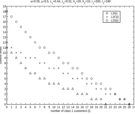
Figure 2.1 illustrates the optimal policies for class 1 customers with parameters α = 0.05, µ= 0.5, λ1 = 0.44, λ2 = 0.01, h1 = 20, h2 = 10, r1 = 200, r2 = 190. Figure
2.2 - 2.6 illustrate the optimal policies for class 2 customers under different arrival rates. Figure 2.2 uses the same parameters as used in Figure 2.1 and shows that LI
2(i) ≤ LC2(i) ≤ LS2(i),∀i. Keeping the other parameters the same, Figure 2.3 uses
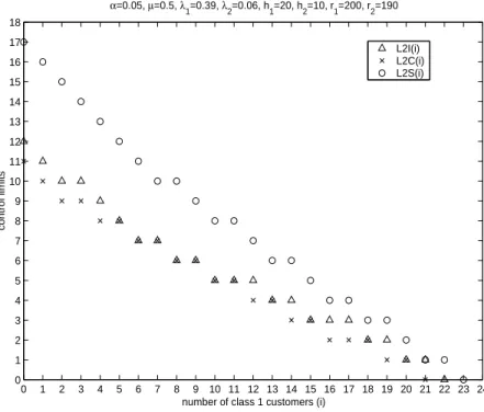
λ1 = 0.39, λ2 = 0.06, and shows that LC2(i) ≤ LI2(i) ≤ LS2(i),∀i. Figure 2.4 uses
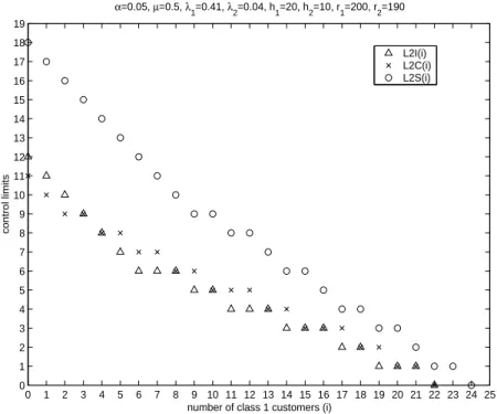
λ1 = 0.27, λ2 = 0.18, and shows that LC2(i) ≤ LS2(i) ≤ LI2(i),∀i. Figure 2.5 uses
λ1 = 0.41, λ2= 0.04, and shows thatLI2(i)≥LC2(i) for i≤4, LI2(i)≤LC2(i) fori≥5.
Figure 2.6 uses λ1 = 0.32, λ2 = 0.13, and shows that LI2(i)≤LS2(i) fori ≤7, LI2(i)≥
LS
2(i) for i ≥ 8. We only change the arrival rates in the above examples. However,
other numerical examples show that changing other parameters may also affect the relative position of LI
2(i). Thus the relationship between the individually optimal
0 1 2 3 4 5 6 7 8 9 10 11 12 13 0
1 2 3 4 5 6 7 8 9 10
number of class 2 customers (j)
control limits
α=0.05, µ=0.5, λ1=0.44, λ2=0.01, h1=20, h2=10, r1=200, r2=190
L1I L1C L1S(j)
Figure 2.1: Class 1 switching curves: LS1(j)≤LC1 ≤LI1
0 1 2 3 4 5 6 7 8 9 10 11 12 13 14 15 16 17 18 19 20 21 22 23 24 25 26 27 0
1 2 3 4 5 6 7 8 9 10 11 12 13 14 15 16 17 18 19
number of class 1 customers (i)
control limits
α=0.05, µ=0.5, λ
1=0.44, λ2=0.01, h1=20, h2=10, r1=200, r2=190
L2I(i) L2C(i) L2S(i)
0 1 2 3 4 5 6 7 8 9 10 11 12 13 14 15 16 17 18 19 20 21 22 23 24 0 1 2 3 4 5 6 7 8 9 10 11 12 13 14 15 16 17 18
number of class 1 customers (i)
control limits
α=0.05, µ=0.5, λ1=0.39, λ2=0.06, h1=20, h2=10, r1=200, r2=190
L2I(i) L2C(i) L2S(i)
Figure 2.3: Class 2 switching curves: LC2(i)≤L2I(i) ≤LS2(i)
0 1 2 3 4 5 6 7 8 9 10 11 12 13 14 15 16 17 18 19 20 21 22 23 24 25 26 27 0 1 2 3 4 5 6 7 8 9 10 11 12 13 14 15 16 17 18
number of class 1 customers (i)
control limits
α=0.05, µ=0.5; λ
1=0.27, λ2=0.18, h1=20, h2=10, r1=200, r2=190
L2I(i) L2C(i) L2S(i)
0 1 2 3 4 5 6 7 8 9 10 11 12 13 14 15 16 17 18 19 20 21 22 23 24 25 0 1 2 3 4 5 6 7 8 9 10 11 12 13 14 15 16 17 18 19
number of class 1 customers (i)
control limits
α=0.05, µ=0.5, λ1=0.41, λ2=0.04, h1=20, h2=10, r1=200, r2=190
L2I(i) L2C(i) L2S(i)
Figure 2.5: Class 2 switching curves: LI2(i)≥LC2(i) for i≤4, LI2(i)≤LC2(i) for i≥5
0 1 2 3 4 5 6 7 8 9 10 11 12 13 14 15 16 17 18 19 20 21 22 23 24 25 26 0 1 2 3 4 5 6 7 8 9 10 11 12 13 14 15 16 17
number of class 1 customers (i)
control limits
α=0.05, µ=0.5, λ
1=0.32, λ2=0.13, h1=20, h2=10, r1=200, r2=190
L2I(i) L2C(i) L2S(i)
Chapter 3
Admission Control: Sample Path
Approach
3.1
Problem Description
In this chapter, we study the multi-priority admission control problem as defined in Chapter 2 with the following two differences: (i) Rewards are generated at the time of service completion instead of the time of joining the repair queue. This shift of reward time changes the nature of the problem in some critical ways, e.g. the optimal value function is no longer non-decreasing in the number of customers of each type in initial state, and the cases where every customer is accepted do not exist anymore. (ii) We prove the structural results using sample path analysis (specifically, the coupling method) (Lindvall [26], Wu et al. [47] ) instead of standard value iteration method as used in Chapter 2. The sample path approach provides more concise proofs.
3.2
Individual Optimization
Following the same approach as the proof of Theorem 1, we can derive the following results for individually optimal policies.
Theorem 10. Under the individual optimization criterion, an arriving class 1
cus-tomer who sees the system in state (i, j) joins the queue if and only if i < LI
1, where
LI
1 =blog
h1
h1+αr1
/log µ
µ+αc. (3.1)
An arriving class 2 customer who sees the system in state (i, j) joins the queue if and only if j < LI
2(i), where
LI
2(i) =
blog h2
(h2+αr2)φi(α)/logβc, if i≤L
I
1
b(log h2
(h2+αr2)φ
LI1(
α) + (i−L
I
1)(log
µ+α
µ ))/logβc, if i > L I
1
(3.2)
where φi(α) is the LST of the busy period initiated by i class 1 customers and β = µ
α+µ+λ1(1−φ1(α)). bxc is the largest integer less than or equal to x. Furthermore, L
I
2(i)
is decreasing in i.
Note that shifting the reward time (from the moment a customer joins the queue to the moment a customer finishes service) not only changes the form of the threshold functions but also eliminates the cases where everyone is accepted.
3.3
Social Optimization
Lippman [27], we uniformize the process by defining the uniform rate Λ =λ1+λ2+µ.
Rescaling time so that Λ +α= 1, we have the following optimality equations
v(i, j) = h1i+h2j+λ1min{v(i, j), v(i+ 1, j)}
+λ2min{v(i, j), v(i, j+ 1)}
+µ
v(i−1, j)−r1, if i≥1
v(0, j−1)−r2, if i= 0, j ≥1
v(0,0), if i= 0, j = 0.
(3.3)
Lemma 9. v(0,1)−v(0,0) +r2 ≥0.
Proof. Define two processes on the same probability space so that they see the same arrivals and potential services. Process 1 starts in state (0,1) and follows optimal policy. Process 2 starts in state (0,0) and follows policy φ which is described below. Let τ be the first time Process 1 reaches state (0,0). Let Process 2 take the same action as Process 1 upon each arrival until time τ, then follow the optimal policy afterwards. If a new class 2 customer is accepted while Process 1 is serving the last class 2 customer, we resample the remaining service time of the class 2 customer currently under service in Process 1 so that he finishes service at the same time as the new class 2 customer in Process 2. (This resampling argument can be applied to similar situations in the rest of this paper.) Therefore, Process 1 and 2 have identical customers except for one extra class 2 customer in Process 1 until time τ. Two processes become identical from then on. Thus,
v(0,1)−v(0,0) ≥ v(0,1)−vφ(0,0)
= E
Z τ
0
e−αth2dt+Ee−ατ(−r2+v(0,0)−v(0,0))
Lemma 10. v is supermodular, i.e.,
v(i+ 1, j+ 1)−v(i+ 1, j)−v(i, j + 1) +v(i, j)≥0. (3.4)
Proof. Fixi and j. Define four processes on the same probability space so that they see the same arrivals and potential services. Process 1 and 4 follow optimal policies and start in states (i+ 1, j+ 1) and (i, j), respectively. Process 2 and 3 start in states (i+ 1, j) and (i, j+ 1), respectively, and use policies φ2 and φ3 which are described
below. Denote the state of Process k at time t by (Xk
t , Ytk), k= 1,2,3,4.
Let τ1 be the first time Process 2 and 3 have 0 customers entirely. Note that if
Process 2 and 3 take the same action upon each arrival they will reach state (0,0) at the same time, since service rates are the same for both classes. Let τ2 be the first
time Process 1 and 4 take different actions. Define τ = min{τ1, τ2}. Let Process 2
and 3 take the same action as Process 1 and 4 until time τ, then follow the optimal policy afterwards. Thus
v(i+ 1, j+ 1)−v(i+ 1, j)−v(i, j+ 1) +v(i, j) ≥ v(i+ 1, j+ 1)−vφ2
(i+ 1, j)−vφ3
(i, j+ 1) +v(i, j)
= E
Z τ
0
e−αt[h(X4
t + 1, Y
4
t + 1)−h(X
4
t + 1, Y
4
t )−h(X
4
t, Y
4
t + 1) +h(X
4
t, Y
4
t )]dt +Ee−ατ(−R1+R2+R3−R4)
+Ee−ατ(v(X1
τ, Yτ1)−v(Xτ2, Yτ2)−v(Xτ3, Yτ3) +v(Xτ4, Yτ4)),
where Ri is the potential reward generated in Process i at time τ. It can be easily seen that the first term is 0 because of the linear holding cost rate.
To simplify notation, define
A=−R1+R2+R3−R4 (3.6)
B =v(Xτ1, Yτ1)−v(Xτ2, Yτ2)−v(Xτ3, Yτ3) +v(Xτ4, Yτ4). (3.7)
Case 1: τ =τ1. Then, at τ, the four processes are in states (0,1), (0,0), (0,0), and
(0,0), respectively. The two distinct paths by which this state is reached are: (i) {(1,2) (1,1) (0,2) (0,1)} → {(0,2) (0,1) (0,1) (0,0)} → {(0,1) (0,0) (0,0) (0,0)}; (ii){(2,1) (2,0) (1,1) (1,0)} → {(1,1) (1,0) (0,1) (0,0)} → {(0,1) (0,0) (0,0) (0,0)}. In the former case,R1 =R2 =R3 =r2, andR4 = 0. In the latter case, R1 =R2 =r1,
R3 =r2, and R4 = 0. In both cases, we have
D≥Ee−ατ(r
2+v(0,1)−v(0,0))≥0,
where the last inequality follows from Lemma 9.
Case 2: τ =τ2. Then A= 0. We have the following possibilities.
Case 2.1: A class 1 arrival is accepted by Process 1 and rejected by Process 4. Let Process 2 accept the arrival and Process 3 reject it. Then after this event the states in four processes are (X4
τ + 2, Yτ4 + 1), (Xτ4 + 2, Yτ4), (Xτ4, Yτ4 + 1), and (Xτ4, Yτ4), respectively. Adding and subtracting v(X4
τ + 1, Yτ4+ 1) +v(Xτ4+ 1, Yτ4), we have
B = v(Xτ4+ 2, Yτ4 + 1)−v(Xτ4+ 1, Yτ4+ 1)−v(Xτ4+ 2, Yτ4) +v(Xτ4+ 1, Yτ4) +v(Xτ4+ 1, Yτ4+ 1)−v(Xτ4, Yτ4 + 1)−v(Xτ4+ 1, Yτ4) +v(Xτ4, Yτ4).
Note that the first four terms and the second four terms above are inequality (3.4) evaluated at (X4
τ + 1, Yτ4) and (Xτ4, Yτ4), respectively. Thus the above argument can be repeated until either Case 1 or Case 2.2 or Case 2.4 happens.
Case 2.2: A class 1 arrival is rejected by Process 1 and accepted by Process 4. Let Process 2 reject the arrival and Process 3 accept it. Then after this event the states in four processes are (X4