LARGE SCALE VISUAL RECOGNITION OF CLOTHING, PEOPLE AND STYLES
M. Hadi Kiapour
A dissertation submitted to the faculty of the University of North Carolina at Chapel Hill in partial fulfillment of the requirements for the degree of Doctor of Philosophy in
the Department of Computer Science.
Chapel Hill 2015
c
2015 M. Hadi Kiapour ALL RIGHTS RESERVED
ABSTRACT
M. HADI KIAPOUR: LARGE SCALE VISUAL RECOGNITION OF CLOTHING, PEOPLE AND STYLES.
(Under the direction of Tamara L. Berg.)
Clothing recognition is a societally and commercially important yet extremely chal-lenging problem due to large variations in clothing appearance, layering, style, body shape and pose. In this dissertation, we propose new computational vision approaches that learn to represent and recognize clothing items in images.
First, we present an effective method for parsing clothing in fashion photographs, where we label the regions of an image with their clothing categories. We then extend our approach to tackle the clothing parsing problem using a data-driven methodology: for a query image, we find similar styles from a large database of tagged fashion images and use these examples to recognize clothing items in the query. Along with our novel large fashion dataset, we also present intriguing initial results on using clothing estimates to improve human pose identification.
able to classify clothing styles and identify the clothing elements are most discriminative in every style.
Finally, we define a new task, Exact Street to Shop, where our goal is to match a real-world example of a garment item to the same exact garment in an online shop. This is an extremely challenging task due to visual differences between street photos that are taken of people wearing clothing in everyday uncontrolled settings, and online shop photos, which are captured by professionals in highly controlled settings. We introduce a novel large dataset for this application, collected from the web, and present a deep learning based similarity network that can compare clothing items across visual domains.
ACKNOWLEDGMENTS
First and foremost, I would like to express my deepst gratitude to my advisor, Pro-fessor Tamara Berg. Her knowledge, enthusiasm, guidance and brilliant ideas have en-lightened my research through these years. Tamara taught me how to be a researcher, identify promising scientific objectives and explore novel directions for research. I am so grateful for the countless hours she spent with me for brainstorming and helping me present my findings. I was also extremely fortunate to collaborate closely with Profes-sor Alex Berg. I feel very grateful to him for his incredible insights, comments and his continuous encouragement from the beginning of my graduate career. Special thanks are also extended to my wonderful thesis committee members: Professor Svetlana Lazebnik, Professor Jan-Michael Frahm, and Dr. Robinson Piramuthu.
to Professor Fred Brooks and Professor Ron Alterovitz for sharing their enthusiasm on teaching in technical communication class.
I am also grateful to all of my industrial collaborators. I spent two summers at eBay Research where I had the chance to collaborate with world-class researchers and engineers. In particular, I would like to thank Dr. Robinson Piramuthu for his leadership and supervision which led me to develop a passion for tackling challenging, open-ended, real-world problems. I am also thankful to Dr. Hassan Sawaf for his extensive support and confidence in my work. Also thanks to all my collaborators during my internships, especially Dr. Wei Di and Dr. Vignesh Jagadeesh.
I want to thank Professor Kota Yamaguchi for being an excellent friend, mentor and a great inspiration for me. I truly appreciate and value everything I have learned from you. I would also like to thank Dr. Kevin Yager for his impressive work in our collaborative research with the Brookhaven National Labs.
Special thanks to Professor Mehrdad Shahshahani for sparking my passion for com-puter vision, his exceptional leadership, support and providing me with the opportunity to conduct research during my undergraduate years. I gratefully thank Professor Ali Farhadi for his supervision and guidance from the very early stages of my research in the area. Thank you to many wonderful professors and colleagues at KTH Royal Institute of Technology in Stockholm, especially Professor Stefan Carlsson and Professor Jan-Olof Eklundh for providing me the opportunity to become a better scientist.
This journey would not have been possible without the support of my family. To my parents, thank you for your endless love and encouraging me in all of my pursuits and
inspiring me to chase my dreams. Thank you uncle Michael and aunt Adele, for your wisdom, kindness and for believing in me. I am so blessed to have you in my life.
TABLE OF CONTENTS
LIST OF FIGURES . . . xii
LIST OF TABLES . . . .xiv
CHAPTER 1: INTRODUCTION . . . .1
1.1 Motivation . . . .1
1.2 Thesis Statement . . . .5
1.3 Outline of Contributions . . . .5
CHAPTER 2: RELATED WORK . . . .8
2.1 Clothing Parsing . . . .8
2.2 Pose Estimation . . . .9
2.3 Semantic Clothing Recognition. . . 10
2.4 Clothing Retrieval . . . 11
2.5 Domain Adaptation and Deep Similarity Learning . . . 12
CHAPTER 3: CLOTHING PARSING . . . 14
3.1 Introduction . . . 14
3.2 CRF Parsing . . . 14
3.2.1 Dataset. . . 15
3.2.2 Problem Formulation. . . 15
3.2.3 Superpixels . . . 17
3.2.4 Pose Estimation . . . 18
3.2.5 Clothing Labeling . . . 18
3.2.6 Training . . . 21
3.2.7 Experimental Results . . . 22
3.2.8 Retrieving Visually Similar Garments . . . 24
3.3 PAPER DOLL PARSING . . . 26
3.3.1 Paper Doll Dataset . . . 27
3.3.2 Paper Doll Parsing Overview. . . 28
3.3.3 Tag prediction. . . 30
3.3.4 Parsing . . . 32
3.3.5 Experimental results . . . 40
3.4 Parsing for Pose Estimation . . . 44
3.5 Summary and Discussion. . . 46
CHAPTER 4: CLOTHING STYLE RECOGNITION. . . 47
4.1 Hipster Wars: Style Dataset and Rating Game . . . 47
4.1.1 Data Collection . . . 47
4.1.2 Rating Game . . . 48
4.1.3 Game Details. . . 51
4.1.4 Game Results . . . 53
4.1.5 Pairwise vs. Individual Ratings . . . 54
4.3 Predicting Clothing Styles. . . 57
4.3.1 Between-class Classification . . . 58
4.3.2 Within-class Classification . . . 59
4.4 Discovering the Elements of Styles . . . 61
4.4.1 General Style Indicators. . . 61
4.4.2 Style Indicators for Individuals. . . 62
4.4.3 Analysis of Style Indicators for Individuals. . . 65
4.5 Summary and Discussion. . . 66
CHAPTER 5: CLOTHING RETRIEVAL . . . 67
5.1 Dataset. . . 69
5.1.1 Image Collection . . . 70
5.1.2 Image Annotation . . . 75
5.2 Approaches . . . 76
5.2.1 Whole Image Retrieval . . . 77
5.2.2 Object Proposal Retrieval . . . 78
5.2.3 Similarity Learning. . . 78
5.2.4 Train/val Sets for Similarity Learning. . . 84
5.3 Experimental Results. . . 84
5.3.1 Human Evaluation . . . 87
5.4 Summary and Discussion. . . 90
CHAPTER 6: SUMMARY AND DISCUSSION. . . 91
LIST OF FIGURES
3.1 Clothing parsing pipeline . . . 17
3.2 Example successful results on the Fahionista dataset . . . 25
3.3 Example failure cases . . . 25
3.4 Prototype garment search application results . . . 26
3.5 Parsing pipeline . . . 28
3.6 Retrieval examples. . . 30
3.7 Tag prediction PR-plot . . . 31
3.8 Parsing outputs at each step. . . 32
3.9 Transferred parse . . . 36
3.10 Parsing examples . . . 41
3.11 F-1 score of non-empty items . . . 41
4.1 Example snapshot of Hipster Wars game . . . 48
4.2 Average image for each style category . . . 49
4.3 Distribution of players across the globe. . . 50
4.4 Example results from our style rating game . . . 54
4.5 Style scores collected by Hipster Wars game. . . 55
4.6 Hipster Wars pairwise vs. individual ratings from Amazon Mech. Turk . . . 56
4.7 Representation of style descriptor . . . 57
4.8 Between-class classification results. . . 58
4.9 Example results of within-classification task . . . 59
4.10 Within-Class classification results . . . 60
4.11 Clothing items across styles. . . 62
4.12 From parts to items . . . 63
4.13 Example predicted style indicators for individuals. . . 65
5.1 Exact street to shop matching . . . 68
5.2 Example street outfit photos . . . 70
5.3 Example shop photos . . . 71
5.4 A snapshot of ModCloth website . . . 72
5.5 Distribution of collected items across shopping sites.. . . 74
5.6 Illustration of category-specific similarity learning . . . 79
5.7 Example retrievals . . . 80
5.8 Our Exact Street to Shop pipeline. . . 82
5.9 Top-k item retrieval accuracy for different numbers of retrieved items.. . . 84
5.10 An example of our human evaluation tasks. . . 88
5.11 Example results of similar-to-item task . . . 89
LIST OF TABLES
3.1 Clothing Parsing performance . . . 23
3.2 Recall for selected garments . . . 24
3.3 Low-level features for parsing. . . 29
3.4 Parsing performance for final and intermediate results . . . 42
3.5 Pose estimation performance with or without conditional parsing input. . . 45
4.1 Human evaluation results for style indicators . . . 66
5.1 Example mappings between keywords and high-level item categories.. . . 77
5.2 Size statistics of the training and validation sets for similarity learning . . . 83
5.3 Dataset statistics and top-20 Exact Street to Shop retrieval accuracy . . . 84
5.4 Human accuracy at choosing the exact matching item . . . 87
CHAPTER 1: INTRODUCTION
1.1 Motivation
Imagine waking up one day to a world where everyone wears the same outfit. What a strange experience would it be? The world would appear much less colorful and interest-ing. Clothing is an integral part of our daily lives, both at the individual and community levels. Choice of clothing communicates a great deal of non-verbal signals that can be interpreted consciously or unconsciously by the observer. In other words, we are what we wear. Our clothing often reveals hints of our wealth, occupation, religion, location and social identity. People purposely select different styles of clothing to wear in different types of social contexts. Fashion is a form of self expression, both to who create it and to the ones who wear it. Understanding clothing is essential to how we perceive the world and form impressions of the ones with whom we engage and interact.
in order to navigate and act in our daily lives. We rapidly and effortlessly recognize ob-jects in various contexts and estimate their geometric relationships even when they are encountered in unusual orientations, under different illumination conditions or partially occluded by other objects in a visually complicated environment. In particular, visual perception plays a fundamental role in the way people form impressions of and make inference about their clothing. People make snap judgements about the aesthetic value of attires. It takes only a glimpse for a person to judge the visual appeal of an outfit or a fashion style. We have an extraordinary cognitive ability to analyze what we see, both at a high level and in finding the most salient constructing elements. Since clothing is generally composed of visual elements, computational vision techniques are the best avenue to automate the exploration of clothing at a large scale. While we highly rely on computers for analyzing large amounts of data, when it comes to visual recognition, human brain far surpasses even the most advanced artificial vision systems. The differ-ence becomes even more evident as one explores complex visual data such as clothing. Clothing produces extremely complex visual patterns, due to large number of possible garment items, large variations in configurations, deformation, appearance, layering, oc-clusion and body poses. While artificial intelligence researchers strive to bridge the gap between human and machine intelligence, a little previous work is devoted to the par-ticular problem of clothing recognition. Our main goal in this thesis is to study and develop scalable computer vision and machine learning systems that learn to represent and identify visual data in order to recognize clothing at a large scale.
To grasp the potential impacts of clothing recognition systems, consider e-commerce.
In 2014, retail e-commerce revenues from apparel and accessories sales amounted to 52.2 billion U.S. dollars and is projected to exceed 80 billion dollars in 20181. Search is an incredibly important part of e-commerce. People go to online marketplaces looking for a specific product or type of clothing. While e-commerce has historically relied heavily on text-based search engines, visual search technology is currently one of the fastest growing and exciting trends in e-commerce. The results of a text-based search engine are only as good as the user’s ability to describe an item and also depends on how well the given keywords match to the product description on the web. In contrast, visual search can provide a significantly more intuitive way to connect with information which leads to more accurate results. Today’s mobile developers strive to build applications that allow customers to snap a photo of a clothing product on the street in the real world and directly search through massive number of products in online shops. This is a very challenging task due to extreme visual differences between real-world photos taken of people wearing clothing in everyday uncontrolled settings, and online shop photos that are taken of clothing items on models, mannequins or in isolation, captured by professionals in highly controlled settings. In addition, highly costumed garment items and unbranded apparels make visual retrieval of clothing even more challenging compared to many other object categories such as electronics.
While search plays a central role in today’s world of commerce, the future of e-commerce relies on adding a sense of discovery to the utilitarian nature of search. Recom-mendation engines and product discovery sites are nowadays among the top fast growing
trends in e-commerce. Targeted discovery, which means guiding consumers to specific products based on their history and personal preferences, creates a custom experience for digital shoppers according to their passions. This is even more important in the clothing and fashion industry, since many desirables are less about search and more about dis-covery. Some examples are “what should I wear with my cowgirl boots?”, “what should I wear to look a bit cooler?” or “what’s the best outfit for the weather today?”. Build-ing artificial intelligence systems that construct complex semantics from the enormous amount of clothing data available online, can be of impressive commoditization value.
With the rise of social networking in the past years, many online communities are formed around connecting people who share the same fashion taste or are passionate about sparing and taking inspirations. Fashion is a fast pace, exciting, transcending field full of creativity. People deeply care about sharing and communicating inspirations visually. Enabling computers to have a sense of current fashion, predict future trends and to understand personal styles can have an exceptional value in numerous applications including categorizing personal or public photo galleries, personalized advertisements, personalized outfit composition, recommendation systems, and matchmaking in online dating platforms.
In this dissertation, we study three main problems, all essential to a comprehen-sive automated clothing recognition system: clothing parsing (Chapter 3), fashion style recognition (Chapter 4) and visual matching of clothing items (Chapter 5).
1.2 Thesis Statement
This thesis addresses the problem of clothing recognition using computational visual representations empowered by machine learning. We introduce effective techniques for representation and identification of clothing in visual data with applications in clothing parsing, recognizing people’s fashion styles and clothing retrieval in large scale.
1.3 Outline of Contributions
In Chapter 3, we propose novel approaches for parsing clothing in fashion pho-tographs, an extremely challenging problem due to the large number of possible garment items, variations in configuration, garment appearance, layering, and occlusion. We first present a probabilistic approach for labeling super pixels in an image with their clothing labels using conditional random fields. Next, we extend our clothing parsing system by using a retrieval-based approach: For every query image, we find similar styles from a large database of tagged fashion images and use these examples to recognize clothing items in the query. Our approach combines parsing from pre-trained global clothing models, local clothing models learned on the fly from retrieved examples, and trans-ferred parse-masks from retrieved examples. We demonstrate a prototype application for pose-independent visual garment retrieval and present intriguing initial results on using clothing estimates to improve pose identification.
human judgments of style. We use this game to collect a new dataset of clothing outfits with associated style ratings for 5 style categories: hipster, bohemian, pinup, preppy, and goth. Next, we train models for between-class and within-class classification of styles. Finally, we explore methods to identify clothing elements that are generally discriminative for a style, and methods for identifying items in a particular outfit that may indicate a style.
In Chapter 5, we define a new task, Exact Street to Shop, where our goal is to match a real-world example of a garment item to the same garment in an online shop. This is an extremely challenging task due to visual differences between street photos (pictures of people wearing clothing, captured in everyday, uncontrolled settings) and online shop photos (pictures of clothing items on people, mannequins, or in isolation, captured by professionals in highly controlled settings). We collect a novel large dataset for this application containing photos from online shops and daily outfit photos. We present our deep learning based similarity network for measuring the similarity between pairs of clothing items across different visual domains.
In summary the novel contributions presented in this thesis are as follows:
• Novel clothing parsing approaches for precise prediction of clothing items and their location in images.
• Large novel dataset for studying clothing parsing, consisting of fashion photos
• Initial experiments on how clothing prediction can improve pose estimation.
• An online competitive rating game to collectively compute style ratings based on
human judgments.
• A new style dataset depicting different fashion styles with associated crowd sourced style ratings.
• Between-class and within-class classification of styles.
• Experiments to identify the outfit elements that are most predictive for a fashion style or within an image.
• Introduction of the Exact Street to Shop task
• A novel large dataset, the Exact Street to Shop Dataset, for street-to-shop clothing retrieval.
• A deep learning based similarity network for the Exact Street to Shop retrieval task.
CHAPTER 2: RELATED WORK
2.1 Clothing Parsing
2013; Liu et al., 2014; Hasan and Hogg, 2010; Scheffler and Odobez, 2011; Yang and Yu, 2011; Gallagher and Chen, 2008; Jammalamadaka et al., 2013; Simo-Serra et al., 2014). In Yang and Yu (2011), clothing recognition is used in surveillance videos. In Hasan and Hogg (2010), they improve the MRF formulation by adding prior models on shape and color of clothing items. In Scheffler and Odobez (2011), the regions around faces are labeled as skin, hair, clothing and background. The work of Wang and Ai (2011) attacks multi-person clothing segmentation in highly occluded images. In Simo-Serra et al. (2014), they incorporate appearance and location priors for each garment, as well as symmetry in their parsing. Dong et al. (2013) introduceParselets, mid-level segments that carry strong semantic information, into parsing. In Chapter 3, we tackle cloth-ing parscloth-ing problem as an object segmentation uscloth-ing CRFs. Our main contribution lies in defining the unary potential, where we use a pose estimation algorithm (Yang and Ramanan, 2011) to model a clothing type. Great performance was obtained when the system was given information about which garment classes, but not their location, are present for each test image. This issue is partially addressed in 3.3, where we utilize over 300 thousand weakly labeled images, where the weak annotations are in the form of image-level tags.
2.2 Pose Estimation
earlier attempts were based on detecting body part (Ramanan, 2006; Andriluka et al., 2009; Marcin and Ferrari, 2009). The work of Yang and Ramanan (2011) uses a mixture model of parts, which jointly captures the spatial relations between part locations and co-occurrence between parts. Mixture models are improved in Johnson and Everingham (2011) to handle much larger quantities of training data. Higher-order spatial correspon-dences were modeled in hierarchical models (Tian et al., 2012). More recently, researchers have successfully deployed deep learning methods for human pose estimation (Toshev and Szegedy, 2014; Pfister et al., 2014; Tompson et al., 2014; Xianjie and Yuille, 2014). Our pose estimation subgoal builds on the method of Yang and Ramanan (2011), where we extend our approach to incorporate clothing parsing in mixture models for improving pose identification.
2.3 Semantic Clothing Recognition
There has been a growing interest in applications of clothing recognition such as learning semantic clothing attributes (Chen et al., 2012; Bossard et al., 2012), identifying people based on their outfits, predicting occupation (Song et al., 2011; Shao et al., 2013), urban tribes (Murillo et al., 2012; Kwak et al., 2013), fashion styles (Kiapour et al., 2014), outfit similarity (Vittayakorn et al., 2015) and outfit recommendations (Liu et al., 2012a). Some recent attempts also aimed to automatically reason about aesthetics and fashionability of clothing in a photograph(Yamaguchi et al., 2014; Simo-Serra et al., 2015). Chen et al. (2015a) investigate the possible effects of New York fashion shows on street-chic images of New Yorkers. Veit et al. (2015) train convolutional neural networks
on large scale co-purchase datasets obtained from online shops to predict what items may go well together. In Jing et al. (2015), they deploy distributed computational platforms to build a large-scale clothing search system for commercial applications.
2.4 Clothing Retrieval
Image retrieval is a fundamental problem for computer vision with wide applicability to commercial systems. Many recent retrieval methods at a high-level consist of three main steps: pooling local image descriptors, such as Fisher Vectors (Perronnin and Dance, 2006; Perronnin et al., 2010b,a) or VLAD (Jegou et al., 2010), dimensionality reduction, and indexing. Lim et al. (2013) used keypoint detectors to identify furniture items by aligning 3D models to 2D image regions. Recently, Gong et al. (2014) proposed a multi-scale orderless pooling scheme on deep CNN activations (Krizhevsky et al., 2012) for indexing that significantly improved the geometric invariance of the final representation over global CNN activations. Generally, these methods work quite well for instance retrieval of rigid objects, but may be less applicable for retrieving the soft, deformable clothing items that are our focus.
Our work in Chapter 5 is inspired by the street-to-shop (Liu et al., 2012b) approach, which tackles the domain discrepancy between street photos and shop photos using sparse representations. However, their approach depends on upper/lower body detectors to align local body parts in street and shop images, which may not be feasible in all types of shop images. They also evaluate retrieval performance in terms of a fixed set of hand-labeled attributes. For example, evaluating whether both the query and shop images depict a “blue, long-sleeved, shirt”. While this type of evaluation may suit some shoppers’ needs, our work aims to findexactlythe same item depicted in a street photo in an online shop.
2.5 Domain Adaptation and Deep Similarity Learning
The concept of adapting models between different dataset domains has been well ex-plored. Many works in this area tackle the domain adaptation problem by learning a transformation that aligns the source and target domain representations into a common feature space (Bell and Kavita, 2015; Fernando et al., 2013; Gopalan et al., 2011; Gong et al., 2012). Other approaches have examined domain adaptation methods for situations where only a limited amount of labeled data is available in the target domain. These methods train classifiers on the source domain and regularize them against the target domain (Bergamo and Torresani, 2010; Saenko et al., 2010). Recently, as deep convolu-tional neural networks are becoming ubiquitous for feature representations, supervised deep CNNs have proved to be extremely successful for the domain adaptation task (Don-ahue et al., 2014; Hoffman et al., 2014; Yosinkski et al., 2014). Our data can be seen as consisting of two visual domains, shop images and street images. Other examples include
CHAPTER 3: CLOTHING PARSING
3.1 Introduction
In this chapter we tackle the problem of clothing parsing in fashion photographs, an extremely challenging problem due to the large number of possible garment items, vari-ations in configuration, garment appearance, layering, and occlusion. We study clothing estimation at a much more general scale than previous works for real-world pictures. We consider a large number (53) of different garment types, e.g. shoes, socks, belts, rompers, vests, blazers, hats, etc., and explore techniques to accurately parse pictures of people wearing clothing into their constituent garment pieces. We also demonstrate a prototype application for pose-independent visual garment retrieval. Furthermore, we also exploit the relationship between clothing and the underlying body pose in two direc-tions: to estimate clothing given estimates of pose, and to estimate pose given estimates of clothing.
3.2 CRF Parsing
clothing item location with respect to body parts. Pairwise potentials incorporate label smoothing, and clothing item co-occurrence.
3.2.1 Dataset
We use Fashionista dataset described in detail in Yamaguchi et al. (2012), useful for training and testing clothing estimation techniques. In this dataset, there are 685 selected photos with good visibility of the full body and covering a variety of clothing items, fully annotated with ground truth clothing labels and pose annotations for 14 body parts. In the ground truth data set, there are 53 different clothing items, of which 43 items have at least 50 image regions. Adding additional labels forhair,skin, andnull (background), gives a total of 56 different possible clothing labels.
3.2.2 Problem Formulation
We formulate the clothing parsing problem as a labeling of image regions. LetIdenote an image showing a person. The goal is to assign a label of a clothing or null (background) item to each pixel, analogous to the general image parsing problem. However, in this work we simplify the clothing parsing problem by assuming that uniform appearance regions belong to the same item, as reported in (Gallagher and Chen, 2008), and reduce the problem to the prediction of a labeling over a set of superpixels. We denote the set of clothing labels byL≡ {li}, wherei∈U denotes a region index within a set of superpixels
U inI, andli denotes a clothing label for region indexed byi(e.g., li =t-shirtorpants).
We take a probabilistic approach to the clothing parsing problem. Within our frame-work, we reduce the general problem to one of maximum a posteriori (MAP) assign-ments; we would like to assign clothing labels based on the most likely joint clothing label assignments under a probability distribution P(L|I) given by the model. However, it is extremely difficult to directly define such a distribution due to the varied visual appearance of clothing items. Therefore, we introduce another variable, human pose configuration, and consider the distribution in terms of interactions between clothing items, human pose, and image appearance. We denote a human pose configuration by
X ≡ {xp}, which is a set of image coordinates xp for body joints p, e.g., head or right
elbow.
Ideally, one would then like to find the joint MAP assignment over both clothing and pose labels with respect to the joint probability distribution P(X, L|I) simultaneously. However, such MAP assignment problems are often computationally intractable because of the large search space and the complex structure of the probabilistic model. Instead, we split the problem into parts, solving the MAP assignment of P(L|X, I) and P(X|I) separately. Our clothing parsing pipeline proceeds as follows:
1. Obtain superpixels {si} from an imageI
2. Estimate pose configuration X using P(X|I) 3. Predict clothes L using P(L|X, I)
4. Optionally, re-estimate pose configuration X using model P(X|L, I)
Figure 3.1 shows an example of this pipeline. We now briefly describe each step and
(a) Superpixels (b) Pose estimation
null shorts shoes purse top necklace hair skin
(c) Predicted Clothing Parse (d) Pose
re-estimation
Figure 3.1: Clothing parsing pipeline: (a) Parsing the image into Superpixels (Arbelaez et al., 2011),(b)Original pose estimation using state of the art flexible mixtures of parts model (Yang and Ramanan, 2011). (c) Precise clothing parse output by our proposed clothing estimation model (note the accurate labeling of items as small as the wearer’s necklace, or as intricate as her open toed shoes). (d) Optional re-estimate of pose using clothing estimates (note the improvement in her left arm prediction, compared to the original incorrect estimate down along the side of her body).
formally define our probabilistic model.
3.2.3 Superpixels
3.2.4 Pose Estimation
We begin our pipeline by estimating pose ˆX using P(X|I):
ˆ
X ∈arg maxX P(X|I). (3.1)
For our initial pose estimate, we make use of (Yang and Ramanan, 2011). In addition to the above terms, this model includes an additional hidden variable representing a type label for pose mixture components,T ≡ {tp}for each body jointp, containing information
about the types of arrangements possible for a joint. Therefore, the estimation problem is written as ( ˆX,Tˆ) ∈ arg maxX,TP(X, T|I). The scoring function used to evaluate
pose (Yang and Ramanan, 2011) is:
lnP(X, T|I)≡P
pwp(tp)Tφ(xp|I) +
P
p,qwp,q(tp, tq)Tψ(xp−xq)−lnZ, (3.2)
where,w are the model parameters, φand ψ are feature functions, and Z is a partition function.
3.2.5 Clothing Labeling
Once we obtain the initial pose estimate ˆX, we can proceed to estimating the clothing labeling:
ˆ
L∈arg maxLP(L|X, Iˆ ). (3.3)
We model the probability distributionP(L|X, I) with a second order conditional random field (CRF):
lnP(L|X, I)≡X
i∈U
Φ(li|X, I) +
X
(i,j)∈V
λ1Ψ1(li, lj)
+ X
(i,j)∈V
λ2Ψ2(li, lj|X, I)−lnZ, (3.4)
where V is a set of neighboring pairs of image regions, λ1 and λ2 are model parameters, and Z is a partition function.
We model the unary potential function Φ using the probability of a label assignment, given the feature representation of the image regionsi:
Φ(li|X, I)≡lnP(li|φ(si, X)). (3.5)
We define the feature vectorφas the concatenation of (1) normalized histograms of RGB color, and (2) normalized histogram of CIE L*a*b* color, (3) histogram of Gabor filter responses, (4) normalized 2D coordinates within the image frame, and (5) normalized 2D coordinates with respect to each body joint location xp. In our experiments, we
use 10 bins for each feature type. Using a 14-joint pose estimator, this results in a 360 dimensional sparse representation for each image region. For the specific marginal probability model P(li|φ(s, X)), we experimentally evaluated a few distributions and
The binary potential function Ψ1 is a log empirical distribution over pairs of clothing region labels in a single image:
Ψ1(li, lj)≡ln ˜P(li, lj). (3.6)
This term serves as a prior distribution over the pairwise co-occurrence of clothing labels (e.g. shirts are near blazers, but not shoes) in neighboring regions within an image. We compute the function by normalizing average frequency of neighboring label pairs in training samples.
The last binary potential in (3.4) estimates the probability of neighboring pairs having the same label (i.e. label smoothing), given their features, ψ:
Ψ2(li, lj|X, I)≡lnP(li =lj|ψ(si,sj, X)). (3.7)
We define the feature transformation to be
ψ(si,sj)≡[(φ(si) +φ(sj))/2,|φ(si)−φ(sj)|] (3.8)
As with the unary potential, we use logistic regression for this probability distribution. Because of the loopy structure of our graphical model, it is computationally in-tractable to solve (3.3) exactly. Therefore, we use belief propagation to obtain an ap-proximate MAP assignment, using the libDAI (Mooij, 2010) implementation.
In practice, regions outside of the bounding box around pose estimation are always
background. Therefore, in our experiment, we fix these outside regions to null and run inference only within the foreground regions.
3.2.6 Training
Training of our parser includes parameter learning of the pose estimator P(X|I) and
P(X|L, I), learning of potential functions inP(L|X, I), and learning of CRF parameters in (3.4).
Pose estimator: The training procedure of (Yang and Ramanan, 2011) uses separate negative examples, sampled from scene images to use the pose estimator as a detector. Since our problem assumes a person is shown, we do not use a scene based negative set, but rather mine hard negative examples using false detections in our images. We treat a detection as negative if less than 30% of the body parts overlap with their true locations with ratio more than 60%.
Potential functions: We learn the probability distributionsP(li|φ) andP(li =lj|ψ)
in (3.5) and (3.7) using logistic regression with L2 regularization (liblinear implementa-tion (Fan et al., 2008a)). For each possible clothing item, e.g. shirt orboots we learn the distribution its regional features,P(li|φ). We learn this model using a one-versus-all
ap-proach for each item. This usually introduces an imbalance in the number of positive vs negative examples, so the cost parameter is weighted by the ratio of positive to negative samples.
using line search and a variant of the simplex method (fminsearch in Matlab). In our experiment, typically both λ1 and λ2 preferred small values (e.g., 0.01-0.1).
3.2.7 Experimental Results
We evaluate the performance of our approach using 685 annotated samples from the Fashionista Dataset (described in Sec 3.2.1). All measurements use 10-fold cross validation (9 folds used for training, and the remaining for testing). Since the pose estimator contains some random components, we repeat this cross validation protocol 10 times.
Clothing Parsing Accuracy
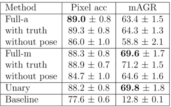
We measure performance of clothing labeling in two ways, using average pixel accu-racy, and using mean Average Garment Recall (mAGR). mAGR is measured by comput-ing the average labelcomput-ing performance (recall) of the garment items present in an image, and then the mean is computed across all images. Table 3.1 shows a comparison for 8 versions of our approach. Full-a and Full-m are our models with CRF parameters learned to optimize pixel accuracy and mAGR respectively (note that the choice of which mea-sure to optimize for is application dependent). The most frequent label present in our images isbackground. Naively predicting all regions to bebackgroundresults in a reason-ably good 77%accuracy. Therefore, we use this as our baseline method for comparison. Our model (Full-a) achieves a much improved89% pixel accuracy, close to the result we would obtain if we were to use ground truth estimates of pose (89.3%). If no pose
Method Pixel acc mAGR Full-a 89.0 ± 0.8 63.4 ± 1.5 with truth 89.3 ± 0.8 64.3 ± 1.3 without pose 86.0 ± 1.0 58.8 ± 2.1 Full-m 88.3 ± 0.8 69.6± 1.7 with truth 88.9 ± 0.7 71.2 ± 1.5 without pose 84.7 ± 1.0 64.6 ± 1.6 Unary 88.2 ± 0.8 69.8± 1.8 Baseline 77.6 ± 0.6 12.8 ± 0.1
Table 3.1: Clothing Parsing performance. Results are shown for our model optimized for accuracy (top), our full model optimized for mAGR (2nd), our model using unary term only (3rd), and a baseline labeling (bottom).
mation is used, clothing parsing performance drops significantly (86%). For mAGR, the Unary model achieves slightly better performance (69.8%) over the full model because smoothing in the full model tends to suppress infrequent (small) labels.
Qualitative evaluation
Garment Full-m with truth without pose
background 95.3±0.4 95.6±0.4 92.5±0.7
skin 74.6±2.7 76.3±2.9 78.4±2.9
hair 76.5±4.0 76.7±3.9 69.8±5.3
dress 65.8±7.7 67.7±9.4 50.4±10.2
bag 44.9±8.0 47.6±8.3 33.9±4.7
blouse 63.6±9.5 66.2±9.1 52.1±8.9
shoes 82.6±7.2 85.0±8.8 77.9±6.6
top 62.0±14.7 64.6±13.1 52.0±13.8
skirt 59.4±10.4 60.6±13.2 42.8±14.5
jacket 51.8±15.2 53.3±13.5 45.8±18.6
coat 30.8±10.4 31.1±5.1 22.5±8.8
shirt 60.3±18.7 60.3±17.3 49.7±19.4
cardigan 39.4±9.5 39.0±12.8 27.9±8.7
blazer 51.8±11.2 51.7±10.8 38.4±14.2
t-shirt 63.7±14.0 64.1±12.0 55.3±12.5
socks 67.4±16.1 67.8±19.0 74.2±15.0
necklace 51.3±22.5 46.5±20.1 16.2±10.7
bracelet 49.5±19.8 56.1±17.6 45.2±17.0
Table 3.2: Recall for selected garments
patterns. Other challenges include pictures with out of frame body joints, close ups of individual garment items, or no relevant entity at all.
3.2.8 Retrieving Visually Similar Garments
We build a prototype system to retrieve garment items via visual similarity in the Fashionista dataset. For each parsed garment item, we compute normalized histograms of RGB and L*a*b* color within the predicted labeled region, and measure similarity between items by Euclidean distance. For retrieval, we prepare a query image and obtain a list of images ordered by visual similarity. Figure 3.4 shows a few of top retrieved results for images displayingshorts,blazer, andt-shirt(query in leftmost col, retrieval results in right 4 cols). These results are fairly representative for the more frequent garment items in the dataset.
null shoes shirt jeans hair skin null tights jacket dress hat heels hair skin null shorts blouse bracelet wedges hair skin null shoes top stockings hair skin Figure 3.2: Example successful results on the Fahionista dataset
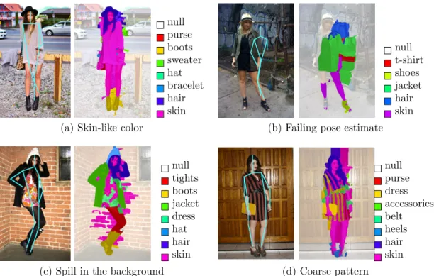
null purse boots sweater hat bracelet hair skin (a) Skin-like color
null t-shirt shoes jacket hair skin (b) Failing pose estimate
null tights boots jacket dress hat hair skin (c) Spill in the background
S
hort
s
Bl
az
er
T-s
hi
rt
Figure 3.4: Prototype garment search application results. Query photo (left column) retrieves similar clothing items (right columns) independent of pose and with high visual similarity.
3.3 PAPER DOLL PARSING
The parsing approach in section 3.2 performed quite well in localization scenarios, where test images are parsed given user provided tags indicating depicted clothing items. However, this approach was less effective at unconstrained clothing parsing, where test images are parsed in the absence of any textual information (detection problem). In this section, we use a large-scale dataset to solve the clothing parsing problem in this challeng-ing detection scenario. We tackle the clothchalleng-ing parschalleng-ing problem uschalleng-ing a retrieval-based approach. For a query image, we find similar styles from a large database of tagged fash-ion images and use these examples to recognize clothing items in the query. Our approach combines parsing from: pre-trained global clothing models, local clothing models learned on the fly from retrieved examples, and transferred parse-masks from retrieved examples.
Furthermore, we provide new experiments evaluating how the resulting clothing parse can benefit the general pose estimation problem.
3.3.1 Paper Doll Dataset
In this approach, we use the Fashionista dataset presented in 3.2.1 and a newly col-lected expansion called the Paper Doll dataset. The Fashionista dataset provides 685 images with clothing and pose annotation that we use for supervised training and perfor-mance evaluation, 456 for training and 229 for testing. The training samples are used to train a pose estimator, learn feature transformations, build global clothing models, and adjust parameters.
Style retrieval Global parse NN parse Transferred Parse Smo ot hi ng Tagged images Input
image Final
parse Parsing
Retrieval
NN
images NN
images NN
images Tag
prediction tags
Figure 3.5: Parsing pipeline. Retrieved images and predicted tags augment clothing parsing.
3.3.2 Paper Doll Parsing Overview
Our parsing approach consists of two major steps:
• Retrieve similar images from the parsed database.
• Use retrieved images and tags to parse the query.
Figure 3.5 depicts the overall parsing pipeline. Section 3.3.3 describes our tag prediction, and Section 3.3.4 details our parsing approach that combines three methods from the retrieval result.
Low-level features
We first run a pose estimator (Yang and Ramanan, 2011) and normalize the full-body bounding box to a fixed size, 302×142 pixels. The pose estimator is trained using the Fashionista training split and negative samples from the INRIA dataset (Dalal and Triggs, 2005). During parsing, we compute the parse in this fixed frame size then warp it back to the original image, assuming regions outside the bounding box are background.
Table 3.3: Low-level features for parsing.
Name Description
RGB RGB color of the pixel.
Lab L*a*b* color of the pixel.
MR8 Maximum Response Filters (Varma and Zisserman, 2005). Gradients Image gradients at the pixel.
HOG HOG descriptor at the pixel (Dalal and Triggs, 2005). Boundary Distance Negative log-distance transform from
the boundary of an image.
Pose Distance Negative log-distance transform from 14 body joints and any body limbs.
Our methods draw from a number of dense feature types (each parsing method uses some subset). Table 3.3 summarizes them.
We compute Pose Distance by first interpolating 27 body joints estimated by a pose estimator (Yang and Ramanan, 2011) to obtain 14 points over body. Then, we compute a log-distance transform for each point. Also we compute log-distance transform of skeletal drawing of limbs (lines connecting 14 points). In total, we get a 15 dimensional vector for each pixel.
accessories boots dress jacket sweater bag cardigan heels shorts top
boots skirt belt pumps
skirt t-shirt flats necklace shirt skirt belt shirt shoes skirt tights skirt top blazer shoes shorts top
skirt belt blazer
boots shorts t-shirt belt dress heels jacket shoes shorts bracelet jacket pants shoes top bag blazer boots shorts top accessories blazer shoes shorts top
Figure 3.6: Retrieval examples. The leftmost column shows query images with ground truth item annotation. The rest are retrieved images with associated tags in the top 25. Notice retrieved samples sometimes have missing item tags.
3.3.3 Tag prediction
We use the style descriptor introduced in Yamaguchi et al. (2013), useful for finding images with similar outfits. The retrieved samples are first used to predict clothing items potentially present in a query image. The purpose of tag prediction is to obtain a set of tags that might be relevant to the query, while eliminating definitely irrelevant items for consideration. Later stages can remove spuriously predicted tags, but tags removed at this stage can never be predicted. Therefore, we wish to obtain the best possible performance in the high-recall regime. Figure 3.6 shows two examples of nearest neighbor retrievals.
Our tag prediction is based on a simple voting approach from KNN. While simple, a
0 0.2 0.4 0.6 0.8 1 0
0.1 0.2 0.3 0.4 0.5 0.6 0.7 0.8 0.9 1
Recall
Precision
KNN@25 KNN@10 Linear
Figure 3.7: Tag prediction PR-plot. KNN performs better in the high-recall regime.
data-driven approach is shown to be effective in tag prediction (Guillaumin et al., 2009). In our approach, each tag in the retrieved samples provides a vote weighted by the inverse of its distance from the query, which forms a confidence for presence of that item. We threshold this confidence to predict the presence of an item.
We experimentally selected this simple KNN prediction instead of other models be-cause it turns out KNN works well for the high-recall prediction task. Figure 3.7 shows performance of linear vs KNN at 10 and 25. While linear classification (clothing item classifiers trained on subsets of body parts, e.g. pants on lower body keypoints), works well in the low-recall high-precision regime, KNN outperforms in the high-recall range. KNN at 25 also outperforms 10.
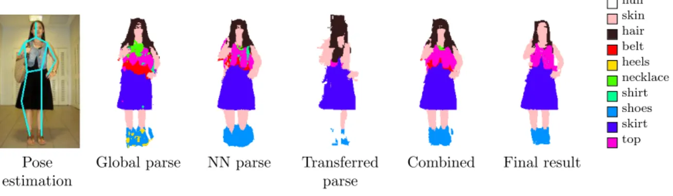
Pose estimation
Global parse NN parse Transferred
parse
Combined Final result
null skin hair belt heels necklace shirt shoes skirt top
Figure 3.8: Parsing outputs at each step. Labels are MAP assignments of the scoring functions.
stage, we always includebackground, skin, and hairin addition to the predicted tags.
3.3.4 Parsing
Following tag prediction, we start to parse the image in a per-pixel fashion. Parsing has two major phases:
1. Compute pixel-level confidence from three methods: global parse, nearest neighbor parse, and transferred parse
2. Apply iterative label smoothing to get a final parse
Figure 3.8 illustrates outputs from each parsing stage.
Pixel confidence
We denote the clothing item label at pixel i by yi. The first step is to compute a
confidence score of assigning clothing iteml toyi. We model this scoring functionSΛ as
the product mixture of three confidence functions.
SΛ(yi|xi, D) ≡ Sglobal(yi|xi, D)λ1 ·
Snearest(yi|xi, D)λ2 ·
Stransfer(yi|xi, D)λ3, (3.9)
where we denote pixel features by xi, mixing parameters by Λ≡[λ1, λ2, λ3], and a set of nearest neighbor samples by D.
Global parse
The first term in our model is a global clothing likelihood, trained for each clothing item on the Fashionista training split. This is modeled as a logistic regression that computes the likelihood of a label assignment to each pixel for a given set of possible clothing items:
Sglobal(yi|xi, D)≡P(yi =l|xi, θlg)·1[l∈τ(D)], (3.10)
whereP is logistic regression given featurexiand model parameterθ g
l,1[·] is an indicator
function, andτ(D) is a set of predicted tags from nearest neighbor retrieval. We use RGB, Lab, MR8, HOG, and Pose Distances as features. Any unpredicted items receive zero probability.
each θgl, we select negative pixel samples only from those images having at least one positive pixel. That is, the model gives localization probability given that a label l is present in the picture. This could potentially increase confusion between similar item types, such as blazer and jacket since they usually do not appear together, in favor of better localization accuracy. We chose to rely on the tag prediction τ to resolve such confusion.
Because of the tremendous number of pixels in the dataset, we subsample pixels to train each of the logistic regression models. During subsampling, we try to sample pixels so that the resulting label distribution is close to uniform in each image, preventing learned models from only predicting large items.
Nearest neighbor parse
The second term in our model is also a logistic regression, but trained only on the retrieved nearest neighbor (NN) images. Here we learn a local appearance model for each clothing item based on examples that are similar to the query, e.g. blazers that look similar to the query blazer because they were retrieved via style similarity. These local models are much better models for the query image than those trained globally (because blazers in general can take on a huge range of appearances).
Snearest(yi|xi, D)≡P(yi =l|xi, θnl)·1[l∈τ(D)]. (3.11)
We learned the model parameterθlnlocally from the retrieved samplesD, using RGB, Lab, Gradient, MR8, Boundary Distance, and Pose Distance.
In this step, we learn local appearance models using predicted pixel-level annotations from the retrieved samples computed during pre-processing detailed in Section 3.3.4. We train NN models using any pixel (with subsampling) in the retrieved samples in an one-vs-all fashion.
Transferred parse
The third term in our model is obtained by transferring the parse-mask likelihoods estimated by the global parse Sglobal from the retrieved images to the query image (Fig-ure 3.9 depicts an example). This approach is similar in spirit to approaches for general segmentation that transfer likelihoods using over-segmentation and matching (Borenstein and Malik, 2006; Leibe et al., 2008; Marsza lek and Schmid, 2012); but here, because we are performing segmentation on people, we can take advantage of pose estimates during transfer.
In our approach, we find dense correspondence based on super-pixels instead of pix-els (Tighe and Lazebnik, 2010) to overcome the difficulty in naively transferring de-formable, often occluded clothing items pixel-wise. Our approach first computes an over-segmentation of both query and retrieved images using a fast and simple segmenta-tion algorithm (Felzenszwalb and Huttenlocher, 2004), then finds corresponding pairs of super-pixels between the query and each retrieved image based on pose and appearance:
Input skin hair jeans shirt jacket boots
skin cardigan dress boots jacket pants
shoes jacket pants Nearest
neighbors Transferred
parse D en se su pe r-p ixe l ma tch in g C on fid en ce tra nsf er
Figure 3.9: Transferred parse. We transfer likelihoods in nearest neighbors to the input via dense matching.
image using L2 Pose Distance.
2. At each super-pixel, compute a bag-of-words representation (Sivic and Zisserman, 2003) for each of RGB, Lab, MR8, and Gradient, and concatenate all.
3. Pick the closest super-pixel from each retrieved image using L2 distance on the concatenated bag-of-words feature.
Let us denote the super-pixel of pixel i by si, the selected corresponding super-pixel
from image r by si,r, and the bag-of-words features of super-pixel s by h(s). Then, we
compute the transferred parse as
Stransfer(yi|xi, D)≡
1
Z
X
r∈D
M(yi, si,r)
1 +kh(si)−h(si,r)k
, (3.12)
where we define
M(yi, si,r)≡
1 |si,r|
X
j∈si,r
P(yi =l|xi, θgl)·1[l ∈τ(r)], (3.13)
which is a mean of the global parse over the super-pixel in a retrieved image. Here we denote a set of tags of image r byτ(r), and the normalization constant byZ.
Combined confidence
After computing our three confidence scores, we combine them with parameter Λ to get the final pixel confidenceSΛas described in Equation 3.9. We choose the best mixing parameter such that MAP assignment of pixel labels gives the best foreground accuracy in the Fashionista training split by solving the following optimization (on foreground pixelsF):
max Λ
X
i∈F
1
˜
yi = arg max
yi
SΛ(yi|xi)
, (3.14)
where ˜yi is the ground truth annotation of the pixeli. For simplicity, we drop the nearest
neighborsDinSΛfrom the notation. We use a simplex search algorithm over the simplex induced by the domain of Λ to solve for the optimum parameter starting from uniform values. In our experiment, we obtained (0.41,0.18,0.39) using the training split of the Fashionista dataset.
which tends to direct the optimizer to find meaningless local optima; i.e., predicting everything as background.
Iterative label smoothing
The combined confidence gives a rough estimate of item localization. However, it does not respect boundaries of actual clothing items since it is computed per-pixel. Therefore, we introduce an iterative smoothing stage that considers all pixels together to provide a smooth parse of an image. Following the approach of Shotton et al. (Shotton et al., 2006), we formulate this smoothing problem by considering the joint labeling of pixels
Y ≡ {yi} and item appearance models Θ≡ {θls}, whereθsl is a model for a label l. The
goal is to find the optimal joint assignment Y∗ and item models Θ∗ for a given image. We start smoothing by initializing the current predicted parsing ˆY0 with the MAP assignment under the combined confidence S. Then, we treat ˆY0 as training data to build initial image-specific models ˆΘ0 (logistic regressions). We only use RGB, Lab, and Boundary Distance since otherwise models easily over-fit. Also, we use a higher regu-larization parameter for training instead of finding the best cross-validation parameter, assuming the initial training labels ˆY0 are noisy.
After obtaining ˆY0 and ˆΘ0, we solve for the optimal assignment ˆYtat the current step
t with the following optimization:
ˆ
Yt∈arg max Y
Y
i
Φ(yi|xi, S,Θˆt)
Y
i,j∈V
Ψ(yi, yj|xi,xj), (3.15)
where we define:
Φ(yi|xi, S,Θˆt)≡ S(yi|xi)λ·P(yi|xi, θsl)1
−λ, (3.16)
Ψ(yi, yj|xi,xj)≡ exp{γe−βkxi−xjk 2
·1[yi 6=yj]}. (3.17)
Here, V is a set of neighboring pixel pairs,λ,β,γ are the parameters of the model, which we set to β = −0.75, λ = 0.5, γ = 1.0 according to perceptual quality in the training images1. We use the graph-cut algorithm (Boykov et al., 2001; Boykov and Kolmogorov, 2004; Kolmogorov and Zabin, 2004) to find the optimal solution.
With the updated estimate of the labels ˆYt, we learn the logistic regressions ˆΘt and
repeat until the algorithm converges. Note that this iterative approach is not guaranteed to converge. We terminate the iteration when 10 iterations pass, when the number of changes in label assignment is less than 100, or the ratio of the change is smaller than 5%.
Offline processing
Our retrieval techniques require the large Paper Doll dataset to be pre-processed (parsed), for building nearest neighbor models on the fly from retrieved samples and for transferring parse-masks. Therefore, we estimate a clothing parse for each sample in the 339K image dataset, making use of pose estimates and the tags associated with the image by the photo owner. This parse makes use of the global clothing models (constrained to the tags associated with the image by the photo owner) and iterative smoothing parts of
our approach.
Although these training images are tagged, there are often clothing items missing in the annotation. This will lead iterative smoothing to mark foreground regions as background. To prevent this, we add an unknown item label with uniform probability and initialize ˆY0 together with the global clothing model at all samples. This effectively prevents the final estimated labeling ˆY to mark missing items with incorrect labels.
Offline processing of the entire Paper Doll dataset took a few days using our Matlab implementation in a distributed environment. For a novel query image, our full parsing pipeline takes 20 to 40 seconds, including pose estimation. The major computational bottlenecks are the nearest neighbor parse and iterative smoothing.
3.3.5 Experimental results
Parsing performance
We evaluate parsing performance on the 229 testing samples from the Fashionista dataset. The task is to predict a label for every pixel where labels represent a set of 56 different categories – a very large and challenging variety of clothing items.
Performance is measured in terms of standard metrics: accuracy, average precision, average recall, and average F-1 score over pixels. In addition, we also include foreground accuracy (See Eq. 3.14) as a measure of how accurately each method is at parsing fore-ground regions (those pixels on the body, not on the backfore-ground). Note that the average measures are over non-empty labels after calculating pixel-based performance for each since some labels are not present in the test set. Since there are some empty predictions,
Input Truth
CRF (Yamaguchi
et al., 2012) Our method Input Truth
CRF (Yamaguchi
et al., 2012) Our method
background blazer cape flats jacket pants scarf socks t-shirt watch
skin blouse cardigan glasses jeans pumps shirt stockings tie wedges
hair bodysuit clogs gloves jumper purse shoes suit tights
accessories boots coat hat leggings ring shorts sunglasses top
bag bra dress heels loafers romper skirt sweater vest
belt bracelet earrings intimate necklace sandals sneakers sweatshirt wallet
Figure 3.10: Parsing examples (best seen in color). Our method sometimes confuses similar items, but gives overall perceptually better results.
0 0.2 0.4 0.6 0.8 1 ba ckg ro un d ski n ha ir acce sso rie s
bag belt
bl aze r bl ou se bo ot s bra ce le t ca pe ca rd ig an cl og s co at dre ss ea rri ng s gl asse s gl ove s hat he el s ja cke t je an s ju mp er le gg in gs ne ckl ace pa nt s pu rse sa nd al s sca rf sh irt sh oe s sh ort s ski rt so cks st ocki ng s su ng la sse s sw ea te r t-sh irt tig ht s
top vest
w at ch w ed ge s CRF Paper Doll
F.g. Avg. Avg. Avg. Method Accuracy Accuracy Precision Recall F-1 CRF (Yamaguchi et al., 2012) 77.45 23.11 10.53 17.20 10.35
Final 84.68 40.20 33.34 15.35 14.87
Global 79.63 35.88 18.59 15.18 12.98
Nearest 80.73 38.18 21.45 14.73 12.84
Transferred 83.06 33.20 31.47 12.24 11.85
Combined 83.01 39.55 25.84 15.53 14.22
Table 3.4: Parsing performance for final and intermediate results (MAP assignments at each step) in percentage.
F-1 does not necessarily match the geometric mean of average precision and recall. Table 3.4 summarizes predictive performance of our parsing method, including a breakdown of how well the intermediate parsing steps perform. For comparison, we in-clude the performance of previous state-of-the-art on clothing parsing (Yamaguchi et al., 2012). Our approach outperforms the previous method in overall accuracy (84.68% vs 77.45%). It also provides a huge boost in foreground accuracy. The previous ap-proach provides 23.11% foreground accuracy, while we obtain 40.20%. We also obtain much higher precision (10.53% vs 33.34%) without much decrease in recall (17.2% vs 15.35%).
In Table 3.4, we can observe that different parsing methods have different strength. For example, the global parse achieves higher recall than others, but the nearest-neighbor parse is better in foreground accuracy. Ultimately, we find that the combination of all three methods produces the best result. We provide further discussion in Section 3.3.5.
Figure 3.10 shows examples from our parsing method, compared to the ground truth annotation and the CRF-based method.We observe that our method usually produces a parse that is qualitatively superior to the previous approach in that it usually respects
the item boundary. In addition, many confusions are between similar item categories, e.g., predicting pants as jeans, or jacket as blazer. These confusions are reasonable due to high similarity in appearance between items and sometimes due to non-exclusivity in item types, i.e.,jeans are a type ofpants.
Figure 3.11 plots F-1 scores for non-empty items (items predicted on the test set) comparing the CRF-based method with our new method. Our model outperforms the previous work on many items, especially major foreground items such as dress, jeans, coat, shorts, or skirt. This results in a significant boost in foreground accuracy and perceptually better parsing results.
Discussion
Though our method is successful at foreground prediction overall, there are a few drawbacks to our approach. By design, our style descriptor aims to represent whole outfit style rather than specific details of the outfit. Consequently, small items like accessories tend to be weighted less during retrieval and are therefore poorly predicted during parsing. This is also reflected in Table 3.4; the global parse is better than the nearest parse or the transferred parse in recall, because only the global parse could retain a stable appearance model of small items. However, in general, prediction of small items is inherently extremely challenging because of limited appearance information.
sometimes contains one item split into two conflicting items.
These two problems are the root of the error in tag prediction – either an item is missing or incorrectly predicted – and result in the performance gap between detection and localization. One way to resolve this would be to enforce constraints on the overall combination of predicted items, but this leads to a difficult optimization problem and we leave it as future work.
Lastly, we find it difficult to predict items with skin-like color or coarsely textured items. Because of the variation in lighting condition in pictures, it is very hard to distinguish between actual skin and clothing items that look like skin, e.g. slim khaki pants. Also, it is very challenging to differentiate for example between bold stripes and a belt using low-level image features. These cases will require higher-level knowledge about outfits to be correctly parsed.
3.4 Parsing for Pose Estimation
In this section, we examine the effect of using clothing parsing to improve pose es-timation. We take advantage of pose estimation in parsing, because clothing items are closely related to body parts. Similarly, we can benefit from clothing parsing in pose estimation, by using parsing as a contextual input in estimation.
We compare the performance of the pose estimator (Yang and Ramanan, 2011), using three different contextual input.
• Baseline: using only HOG feature at each part.
Table 3.5: Pose estimation performance with or without conditional parsing input. Average precision of keypoints (APK)
Method Head Shoulder Elbow Wrist Hip Knee Ankle Mean
Baseline 0.9956 0.9879 0.8882 0.5702 0.7908 0.8609 0.8149 0.8440 Clothing 1.0000 0.9927 0.8770 0.5601 0.8937 0.8868 0.8367 0.8639 - Ground truth 1.0000 0.9966 0.9119 0.6411 0.8658 0.9063 0.8586 0.8829 Foreground 1.0000 0.9926 0.8873 0.5441 0.8704 0.8522 0.7760 0.8461 - Ground truth 0.9976 0.9949 0.9244 0.5819 0.8527 0.8736 0.8118 0.8624
Percentage of correct keypoints (PCK)
Method Head Shoulder Elbow Wrist Hip Knee Ankle Mean
Baseline 0.9956 0.9891 0.9148 0.7031 0.8690 0.9017 0.8646 0.8911 Clothing 1.0000 0.9934 0.9127 0.6965 0.9345 0.9148 0.8843 0.9052 - Ground truth 1.0000 0.9978 0.9323 0.7467 0.9192 0.9367 0.9017 0.9192 Foreground 1.0000 0.9934 0.9148 0.6878 0.9127 0.8996 0.8450 0.8933 - Ground truth 0.9978 0.9956 0.9389 0.7183 0.9105 0.9214 0.8734 0.9080
• Clothing: using a histogram of clothing in addition to HOG feature.
• Foreground: using a histogram of figure-ground segmentation in addition to HOG feature.
Here we concatenate all features into a single descriptor and learn a max-margin linear model (Yang and Ramanan, 2011). All models use 5 mixture components in this exper-iment. We compute the foreground model simply by treating non-background regions in clothing parsing as foreground. Comparing the clothing model and the foreground model reveals how semantic information helps pose estimation compared to non-semantic seg-mentation. We use the Fashionista dataset in this comparison, with the same train-test split described in Section 3.3.1.
also compare the performance when we use the ground-truth pixel annotation, which serves as an upper bound on performance for each model given a perfect segmentation. Clearly, introducing clothing parsing improves the quality of pose estimation. Further-more, the improvement of the clothing model over the foreground model indicates that the contribution is coming from the inclusion of semantic parsing rather than from a simple figure-ground segmentation.
From these performance numbers we can see that clothing parsing is particularly effective for improving localization of end parts of the body, such as the wrist. Perhaps this is due to items specific to certain body parts, such as skin for wrist and shoes for ankle. Note that a figure-ground segmentation cannot provide such semantic context. This result gives an important insight into the pose estimation problem, since improving estimation quality for such end parts is the key challenge in pose estimation, while state-of-the-art methods can already accurately locate major parts such as head or torso. We believe that semantic parsing provides a strong context to improve localization of minor parts that often suffer from part articulation.
3.5 Summary and Discussion
In this chapter, we described novel approaches for clothing parsing. Our experimental results indicate that our data-driven approach is particularly beneficial in the detection scenario, where we need to both identify and localize clothing items without any prior knowledge about depicted clothing items. We also empirically show that pose estimation can benefit from the semantic information provided by clothing parsing.
CHAPTER 4: CLOTHING STYLE RECOGNITION
The clothing we wear and our identities are closely tied, revealing to the world clues about our wealth, occupation, and socio-identity. In this chapter, we examine questions related to what our clothing reveals about our personal style. We first design an online competitive Style Rating Game called Hipster Wars to crowd source reliable human judgments of style. We use this game to collect a new dataset of clothing outfits with associated style ratings for 5 style categories: hipster, bohemian, pinup, preppy, and goth. Next, we train models for between-class and within-class classification of styles. Finally, we explore methods to identify clothing elements that are generally discriminative for a style, and methods for identifying items in a particular outfit that may indicate a style.
4.1 Hipster Wars: Style Dataset and Rating Game
To study style prediction we first collect a new dataset depicting different fashion styles (Section 4.1.1). We then design a crowd-sourcing game called Hipster Wars to elicit style ratings for the images in our dataset (Section 4.1.2).
4.1.1 Data Collection
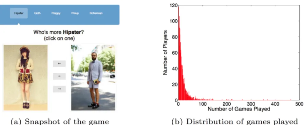
Figure 4.1: Left shows an example game for the hipster category on Hipster Wars. Users click on whichever image is more hipster or click “=” for a tie. Right shows the number of games played per player.
Search using each style name and download top ranked images. We then use Google’s “Find Visually Similar Images” feature to retrieve thousands of additional visually similar images to our seed set and manually select images with good quality, full body outfit shots. We repeat this process with expanded search terms, e.g. “pinup clothing” or “pinup dress”, to collect 1893 images in total. The images exhibit the styles to varying degrees. Average images for each style category is shown in Figure 4.2.
4.1.2 Rating Game
We want to rate the images in each style category according to how strongly they depict the associated style. As we show in section 4.1.5, simply asking people to rate individual images directly can produce unstable results because each person may have a different internal scale for ratings. Therefore, we develop an online game to collec-tively crowd-source ratings for all images within each style category. A snapshot of the game is shown in Figure 4.1. Our game was released to great success, attracting over
Figure 4.2: Average image for each style category
1700 users who provided over 30,000 votes at the time of analysis and the number of votes is growing every day. Our players are also scattered around the globe. Figure 4.3 presents the percentage of players from each continent. While the majority of players are from Americas (74.57%), players from Europe contribute significantly to the game as well (17.53%). Asia, Oceania and Africa constitute a smaller fraction (7.9%) of players together.
Our game is designed as a tournament where a user is presented with a pair of images from one of the style categories and asked to click on whichever image more strongly depicts the solicited style, or to select “Tie” if the images equally depict the style. For example, for images in the hipster category the user would be asked “Who’s more hipster?” After each pair of images, the user is provided with feedback related to the winning and losing statistics of the pair from previous rounds of the tournament.