FLEXIBLE CLASSIFICATION TECHNIQUESWITH
BIOMEDICAL APPLICATIONS
Chong Zhang
AdissertationsubmittedtothefacultyoftheUniversityofNorthCarolinaatChapelHillinpartial fulfillmentoftherequirementsforthedegreeofDoctorofPhilosophyintheDepartmentofStatisticsand
OperationsResearch.
Chapel Hill 2014
Approved by:
Yufeng Liu
Steve Marron
Andrew Nobel
Donglin Zeng
c
ABSTRACT
Chong Zhang: FLEXIBLE CLASSIFICATION TECHNIQUES WITH BIOMEDICAL APPLICATIONS
(Under the direction of Yufeng Liu)
Classification problems are prevalent in many scientific disciplines, especially in biomedical
re-search. Recently, margin based classifiers have become increasingly popular, partly due to their
ability in handling large scale problems with fast computational speed and desirable theoretical
prop-erties. Despite the success of margin based classifiers, many challenges remain. For example, in
practical problems, it can be desirable to estimate the class conditional probability accurately. For
high dimensional classification data, penalized margin based classifiers are commonly used. However,
when estimating the class conditional probability, the shrinkage effect from the penalty term in the
corresponding optimization is often ignored. This effect can lead to large bias in estimation of the
class conditional probability. Another important issue on classification is the comparison between
soft and hard classifiers for multicategory problems. Moreover, regular multicategory margin based
classifiers can suffer from inefficiency by using too many classification functions. In this dissertation,
we propose several new classification techniques to overcome the challenges mentioned above.
Com-prehensive numerical and theoretical studies are presented to demonstrate the usefulness of our new
proposed methodologies.
ACKNOWLEDGMENTS
I would like to thank my advisor Professor Yufeng Liu for his help and encouragement on my
research. Working with him has brought so much fun and valuable experience. I have learned much
through his supportive and encouraging guidance. It is a great pleasure to have him as my advisor.
I am also grateful to the Department of Statistics and Operations Research for providing a
sup-portive and stimulating research environment. I would like to thank all the committee members, who
have provided valuable suggestions and help in my dissertation. I thank all my friends at UNC for
their friendship and help.
TABLE OF CONTENTS
1INTRODUCTION. . . . 1
1.1 Some Background on Classification. . . . 1
1.1.1Binary Classification and Large Margin Classifiers . . . 1
1.1.2 G eneralization to Multicategory Classification . . . .3
1.1.3 C lass Conditional Probability Estimation. . . .5
1.2 N ew Contributions and Outline. . . .6
2 SHRINKAGE ON PROBABILITY ESTIMATION. . . .. . . .8
2.1 Introduction. . . .8
2.2Largemarginclassifiersandt hes hrinkageeffect. . . 10
2.2.1Frameworkof largemarginclassifiers. . . 10
2.2.2Theoreticalpropertyofs hrinkage. . . .13
2.2.3Extension to weighted learning. . . .. . . .16
2.3 A new refit method for probability estimation . . . .18
2.3.1The refit procedure. . . .18
2.3.2 Theoretical properties . . . .20
2.4 Simulation. . . .21
2.5 Real data . . . 22
2.6 Possible future work . . . 24
2.7 Proofs. . . 25
3 MULTICATEGORY LUM.. . . .27
3.1 Introduction . . . 27
3.2 Methodology. . . .29
3.2.1 Background on Binary Classification . . . 29
3.2.2 Existing Multicategory Classification Methods . . . 30
3.2.3 MLUM Family. . . .32
3.3 Statistical Properties. . . .34
3.3.1 Fisher Consistency . . . 35
3.3.2 Probability Estimation. . . 36
3.3.3 Asymptotic Properties. . . 39
3.4 Computational Algorithm . . . .43
3.5 Simulated Examples. . . .45
3.5.1 When Hard Classification is Better . . . 46
3.5.2 When Soft Classification is Better . . . 50
3.5.3 When MLUM with c=1 is Better . . . 51
3.5.4 Summary of Simulation Results. . . 54
3.6 Real Data Examples. . . 56
3.6.1 Benchmark Data. . . 56
3.6.2 Glioblastoma Multiforme Cancer Data. . . 61
3.7 Summary and Possible Future Work . . . .62
3.8 Proofs. . . .. . . .64
4 MULTICLASS ANGLE-BASED CLASSIFIER . . . .69
4.1 Introduction . . . .69
4.2 Methodology. . . 70
4.3 Statistical Properties. . . 73
4.3.1 Fisher Consistency and Theoretical Minimizer. . . 73
4.3.2 Class Conditional Probability Estimation. . . 75
4.3.3 Asymptotic Results . . . 76
4.3.4 Finite Sample Error Bound. . . 81
4.3.5 Comparison to Existing Methods . . . 82
4.4 Computational Algorithms and Tuning Procedures . . . 83
4.5 Simulation Examples. . . 85
4.6 Real Data Examples . . . ..87
4.8 Apendix. . . .. . . .88
5REINFORCED ANGLE-BASED SVM .. . . . 100
5.1 Introduction. . . 100
5.2 Methodology . . . 101
5.3 Fisher Consistentcy. . . 103
5.4 Algorithm.. . . .10 4 5.4.1 Linear Learning. . . .104
5.4.2 Kernel Learning . . . 106
5.4.3 Weighted Learning . . . 108 5.5 Numerical Results. . . .109
5.5.1 Simulated Examples . . . 109.
5.5.2 Real Data Analysis. . . 110
5.6 Discussion and Future Direction.. . . 111
5.7 Proofs. . . 112
BIBLIOGRAPHY. . . 115
1.1SomeBackgroundonClassification
Classification is a typical supervised learning task and it is commonly seen in practice. Given a training
dataset that has both the predictors and labels available, a classifier builds a model and predicts the
label for new instances with only the predictors known. In this section, we briefly review some
fundamental classification techniques and related concepts. In Section 1.1.1, some basic background
of binary classification techniques in the statistical machine learning literature is introduced, and we
focus on the large margin classifiers. We discuss the idea of extending large margin classification
from binary to multicategory learning in Section 1.1.2. In Section 1.1.3, we consider the estimation
problem of class conditional probabilities, which is another important aspect of classification besides
the label prediction.
1.1.1 Binary Classification and Large Margin Classifiers
One important goal of classification is to minimize the prediction error rate. In particular, let the
training data be {(xi, yi);i= 1, . . . , n},i.i.d. from a fixed but unknown distribution P(X, Y), where
X ∈ Rp is a p-dimensional vector of predictors and Y is the corresponding label. A classification
technique builds a model on the training dataset and yields a prediction rule ˆY(X), where ˆY(X)
denotes the predicted label of X. Then, for a new instance with only x observed, we use ˆY(x) as
its prediction. The corresponding prediction error rate can be expressed as EP(X,Y) I( ˆY(X) 6=Y) ,
where I(·) is the indicator function.
There are many classification techniques available in the literature. Well known classification
methods include nearest-neighbors, linear discriminant analysis, logistic regression, tree based method,
and many others. For the nearest-neighbors method, or sometimes referred to as the
k-nearest-neighbors, the class label of x is determined by the majority of y’s of k data points that are the
closest to x. Linear discriminant analysis assumes that the marginal distribution of each P(X|Y) is
normal, and estimates the parameters of the density by the observed data. Then for a new x, we
is the maximum. Logistic regression method models the log-odds of a data point as a function of x,
and find the corresponding maximum likelihood estimator. With the estimated parameters at hand,
the prediction rule is to assign the label with the corresponding maximum probabilities. For tree
based methods, one splits the space ofxinto a set of rectangles. Within each rectangle, the predicted
label is the same as that of the majority of observations in that rectangle. See Hastie, Tibshirani and
Friedman [2009] for a comprehensive review of various methods.
The classifiers aforementioned often work well in the traditional setting where we only have a
relatively small number of predictors. With the advance of technology, the dimensionality of modern
data in various scientific fields keeps increasing. Such high dimensional and complex data pose
challenges for the development of suitable statistical techniques. There are various extensions of
those methods mentioned above. In this dissertation, we focus on a set of machine learning based
classification techniques, namely the large margin classifiers, that can handle high dimensional data
well.
In the literature of large margin classification, where the terminology of large margin is to be
defined below, one assumes that Y ∈ {+1,−1}. To classify the instances, typically one mapsX onto
the real lineRthrough a classification functionf(X), and the corresponding prediction rule is ˆY = +1
iff(X)≥0, and ˆY =−1 iff(X)<0. We assume the classification functionf(·) belongs to a certain
functional class F. For example, one can considerF as a class of linear functionsf(X) =XTβ+β0,
where βis a parameter vector of length pand β0 is the intercept.
To minimize the expected prediction error rate EP(X,Y) I( ˆY(X) 6= Y)
, we may consider its
empirical approximation
min f∈F
1 n
n X
i=1
I(sign(f(xi))6=yi),
or equivalently,
min f∈F
1 n
n X
i=1
I(yif(xi)≤0). (1.1)
Note that in (1.1),I(·) depends onyandf(x) only through their productyf(x). This productyf(x),
called the functional margin, plays an important role in a large margin classification technique. In
particular, for a data point (x, y), the classification is correct if and only ifyf(x)>0. Classification
methods that are based on the functional margin yf(x) are referred to as large margin classifiers.
The optimization problem (1.1) is typically NP-hard, hence it is common to apply a surrogate
loss function `(·) in place of the indicator functionI(·), plus a penalty term on f. The optimization
problem can thus be written in aloss +penalty form
min f∈F
1 n
n X
i=1
`(yif(xi)) +λJ(f). (1.2)
HereJ(f) is the regularization term, or sometimes referred to as the penalty term onf, which prevents
it from overfitting, andλserves as a balance between the loss and the penalty term. A proper choice
of λis crucial in practice.
Different choices of the loss function ` lead to different binary large margin classifiers. To list a
few, AdaBoost in Boosting [Freund and Schapire, 1997; Friedman, Hastie and Tibshirani, 2000] is
shown to be approximately using the exponential loss `(u) = exp(−u), Penalized Logistic Regression
[Lin et al., 2000] uses the deviance loss `(u) = log(1 + exp(−u)), Support Vector Machines (SVMs,
Boser, Guyon and Vapnik [1992]) are equivalent to using the hinge loss`(u) = (1−u)+, and Proximal
SVMs [Fung and Mangasarian, 2001; Suykens and Vandewalle, 1999; Tang and Zhang, 2005] use
`(u) = (1−u)2. See Hastie, Tibshirani and Friedman [2009] for more discussions. Many of these
large margin classifiers are shown to be very useful in practice, and the theoretical properties of
these methods are well studied (see, among others, Steinwart and Scovel [2007], Blanchard, Bousquet
and Massart [2008], Zhang [2004b], Bartlett, Jordan and McAuliffe [2006] and Shawe-Taylor and
Cristianini [2004]).
In the next section, we introduce some extensions of binary classifiers for multicategory problems.
The techniques for a multicategory classifier can be generalized from a binary one in many different
ways, and we give a brief review of some existing multicategory classification methods.
1.1.2 Generalization to Multicategory Classification
In Sections 1.1.1, the focus has been on binary classification methods, especially the large margin
classifiers. We first introduce how to extend binary large margin classification techniques to the
multicategory case with the response variable consisting of more than two classes.
{1, . . . , k}, where k is the number of classes. Similar as the binary case, we need to minimize the
prediction error rate EP(X,Y) I( ˆY(X) 6= Y)
. A natural idea for generalization is to employ a
sequence of binary classifiers for the multicategory problem. There are two major approaches in this
framework, namely, the one-versus-one and one-versus-rest methods.
The one-versus-one approach builds binary classifiers between classesiandj, for all different pairs
ofi, j∈ {1, . . . , k}. Withk(k−1)/2 classifiers at hand, the prediction rule is based on a majority vote.
In particular, a new instance xis labeled as class 1, if it is predicted as class 1 more often than the
other classes among thek(k−1)/2 prediction results. When there is a tie, one may need to use random
guessing to make a decision. The one-versus-rest approach takes class ias the positive class, and all
other classes as the negative one, and trains kdifferent classifiers. When a new instance is available,
the prediction rule is to runkclassifiers and choose the one that has the largest classification function
value. The one-versus-rest approach may suffer from inconsistency when there is no dominating class
for certain large margin classifiers such as the SVM [Liu and Yuan, 2011]. Hence it is desirable to
study a classifier that takes all classes into consideration simultaneously.
For simultaneous multicategory large margin classification, one often aims to calculate a
k-dimensional classification function vector f(X) = (f1(X), . . . , fk(X))T, where f belongs to some
certain functional classF of interest. The prediction rule is ˆY(X) = argmaxj∈{1,...,k}fj(X). Because
of the argmax rule, if we add a constant to each element in f, the prediction does not change. To
overcome this difficulty and to reduce the dimension of the problem, it is common to impose a
sum-to-zero constraint on f. Namely, we restrict f such that Pkj=1fj(X) = 0 for all X. Many existing
simultaneous classifiers follow this framework. See for example, Vapnik [1998], Crammer et al. [2001],
Lee, Lin and Wahba [2004], Zhu and Hastie [2005], Liu and Shen [2006], Tang and Zhang [2006], Zhu
et al. [2009], Liu and Yuan [2011] and Zhang and Liu [2013]. However, although the sum-to-zero
constraint helps to ensure identifiability of the solution, it makes the computational problem more
complex. In Chapter 4, we propose a new simplex based multicategory classification structure that
is free of the sum-to-zero constraint, and hence it enjoys a faster computational speed.
In Section 1.1.3, we will discuss the issue ofclass conditional probability estimation.
1.1.3 Class Conditional Probability Estimation
In this section, we introduce the definition of class conditional probability for a binary case. The
gener-alization to the multicategory case will be discussed later. In practice, besides accurate classification,
an appropriate estimation of the class conditional probability can be important as well.
Recall from the previous section that we assume the data are i.i.d. from P(X, Y). For a given
X = x, suppose that, without loss of generality, P(x, Y = +1) +P(x, Y = −1) > 0. We define
the probability P(Y = +1|X =x) = P(x,Y=+1)+P(x,YP(x,Y=+1) =−1) to be the class conditional probability of
the positive class. The class conditional probability of the negative class can be defined in a similar
manner. Intuitively, this class conditional probability indicates the chance of Y being in class +1 for
a given predictor x. In certain practical problems, an accurate estimation of the class conditional
probability may help to provide more information on how confident the classification is.
We will explore the effect of the penalty term J(f) on the estimation of class conditional
prob-abilities in Chapter 2. In particular, we show that the penalty term tends to shrink the probability
estimation towards 1/2 in binary cases, and we propose a simple refit procedure that helps to correct
the bias.
In the literature of large margin classification, there exists two major groups, called the soft
and hard classifiers Wahba [1999, 2002]. The essential difference between soft and hard classifiers is
whether one needs to estimate the class conditional probability for the classification task or not. In
particular, soft classifiers predict the label based on the obtained class conditional probabilities, while
hard classifiers bypass the estimation of probabilities and focus on the decision boundary. In practice,
for the goal of accurate classification, it is unclear which one to use in a given situation.
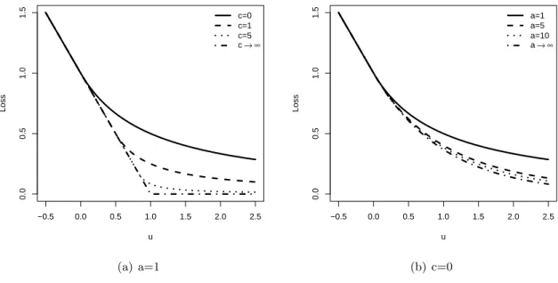
Recently, Liu, Zhang and Wu [2011] proposed a family of binary loss functions, namely the the
Large-margin Unified Machines (LUM), that embraces many existing loss functions as special cases.
In particular, the LUM loss can be expressed as
`(u) =
1−u ifu < 1+cc
1 1+c
a (1+c)u−c+a
a
ifu≥ c 1+c,
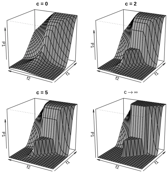
with c ≥ 0 and a > 0 being parameters of the LUM family. Note that the LUM family includes
and Ahn [2007]) with c = 1 and a = 1, as special cases. When c = 0, the classifier is a typical
soft classifier which provides complete class conditional probability information. As c increases, the
probability information becomes more vague. As c→ ∞, it becomes the SVM which only estimates
the classification boundary {x :P(Y = +1|X =x) = 0.5}. The LUM loss function can be used to
study the transition behavior from soft to hard classifiers. Liu, Zhang and Wu [2011] showed that for
binary problems, an accurate estimation of class conditional probability can sometimes help to build
a more accurate classifier, while in some other cases focusing on the classification boundary only may
help to establish a more accurate classifier. We will extend this idea to multicategory problems in
Chapter 3.
1.2 New Contributions and Outline
In this dissertation, we will investigate various aspects of large margin classifiers. We investigate the
role of class conditional probability as well as its estimation. Furthermore, we will propose some new
large margin classification techniques. The main outline of the dissertation is as follows:
In Chapter 2, we investigate the problem of probability estimation for binary large margin
classifiers and illustrate the resulting bias on class probability estimation caused by shrinkage.
We show that such bias can be large for finite sample problems. As a result, modifications are
needed. We propose a simple refit method [Zhang, Liu and Wu, 2013] that helps to correct the
scale problem introduced by shrinkage and yields accurate class probability estimation.
In Chapter 3, we tackle the problem of hard and soft classifiers in multicategory classification
problems. The LUM family, proposed in Liu, Zhang and Wu [2011], enables one to study
the behavior change from soft to hard binary classifiers. For multicategory cases, however,
the concept of soft and hard classification becomes less clear. In that case, class probability
estimation becomes more involved as it requires estimation of a probability vector. We generalize
the idea in Liu, Zhang and Wu [2011] and propose a new Multicategory LUM [MLUM, Zhang
and Liu, 2013] framework to investigate the behavior of soft versus hard classification under
multicategory settings.
In Chapter 4, we propose a new group of simultaneous multicategory large margin
classifica-tion techniques. Among existing simultaneous multicategory extensions, a common one is to
learn kdifferent functions for a k class problem together with a sum-to-zero constraint on the
functions. Such a formulation can be inefficient for multicategory learning. In this chapter, we
propose a new Multicategory Angle-based large margin Classification [MAC, Zhang and Liu,
2014] technique. The proposed MAC associates different classes with vertices of a standard
simplex. The prediction rule is to assign the class label that corresponds to the vertex whose
angle with respect to the classification function is the smallest. All binary large margin
clas-sifiers can be naturally generalized to simultaneous multicategory clasclas-sifiers through the MAC
structure. MAC is free of the commonly used sum-to-zero constraint, and consequently enjoys
more efficient computation.
In Chapter 5, we propose a new multicategory support vector machine under the angle based
framework. The new machine overcomes the difficulty that the regular angle based support
vector machine is Fisher inconsistent. In particular, we propose to use the idea of convex
combination of loss functions as in Liu and Yuan [2011]. We show that with appropriately
chosen penalty, the corresponding optimization can be solved using the coordinate descent
CHAPTER 2: SHRINKAGE ON PROBABILITY ESTIMATION
2.1 Introduction
In classification problems, the classification accuracy is one of the most important measures of
classi-fication performance. An accurate classifier can produce good prediction of class membership for new
subjects. Another important issue is class probability estimation. As there are random errors involved
in the class prediction, class probability estimation gives users information on how strong the evidence
of classifying one subject into a particular class is. The problem of class probability estimation can
be even more important than classification accuracy. For example, in disease diagnosis, it is vital for
doctors and patients to know the chance of a certain disease instead of just a prediction. For two
patients classified into the disease positive class, if their respective class probabilities are 0.501 and
0.999, the probability information is undoubtedly critical.
Our focus is on margin-based, sometimes called large margin, classification techniques. Such
techniques can typically be written as a regularization problem of minimizingLoss +Penalty. Here,
the loss term is used to ensure goodness of fit of the resulting model on the training data. The
penalty term, also known as the regularization term, prevents overfitting through shrinkage so that
the resulting model can produce accurate predictions. Many important classification techniques fit
into the regularization framework, for example, Penalized Logistic Regression [PLR, Lin et al., 2000],
AdaBoost in Boosting [Freund and Schapire, 1997; Friedman, Hastie and Tibshirani, 2000], Import
Vector Machine [Zhu and Hastie, 2005], Proximal SVM [PSVM, Fung and Mangasarian, 2001; Suykens
and Vandewalle, 1999; Tang and Zhang, 2005],ψ-learning [Shen et al., 2003], and more recently,
Large-margin Unified Machines [Liu, Zhang and Wu, 2011]. The regularization term is especially important
for high dimensional data analysis.
One can use the loss function, or sometimes the related likelihood function, to derive a formula for
probability estimation using the classification function. For example, in PLR, one can use the logit
transformation, i.e., the link function between the classification function and the class conditional
probability estimator converges to the true probability as the training sample size gets large. It is
common in practice to use such an estimator of probability, without taking the shrinkage effect into
account. In this chapter, we demonstrate that when the sample size n is relatively small compared
to the dimension p, the shrinkage effect can be very large on probability estimation. In practice,
such probability estimators can have sizeable biases and consequently may give misleading results.
Our goal is to explore the shrinkage effect on classification and more importantly on probability
estimation. Through theoretical studies, we demonstrate how shrinkage affects probability estimation
in binary classification problems. In particular, we show that shrinkage tends to force the resulting
naive probability estimator towards 1/2 in standard learning, where both classes are treated equally.
Inspired by this phenomenon, we explore new methods to achieve better probability estimation. Our
proposed refit method is shown to give consistent probability estimation, and works remarkably well
in the numerical examples. For illustration, we focus on PLR and PSVM in this chapter, however,
our idea is applicable to general margin-based classifiers as well.
In Section 2.2, we review large margin classification techniques and explore some theoretical
properties of shrinkage for several methods. Our results shed some light on poor probability estimation
without adjusting the shrinkage effect. Both standard and weighted learning settings are considered.
In Section 3, we propose a new two-stage refit method for better probability estimation. Given
the classification function of the penalized method from the first step, we refit the classifier as a
one-dimensional problem without penalization to correct the shrinkage bias. We show that the refit method
often has a large gain in probability estimation, while keeping similar classification performance
to the first step. Some asymptotic consistency results of the refit procedure are provided as well.
In Section 2.4, we use simulated examples to examine the performance of the refit approach. In
Section 2.5, we evaluate the methods on two real data examples. Some discussion is provided in
Section 2.6. All technical proofs are collected in Section 2.7.
2.2 Large margin classifiers and the shrinkage effect
2.2.1 Framework of large margin classifiers
In supervised learning, we have a training data set {(xi, yi);i= 1, . . . , n} which contains n
yi the response variable. The dimensionality of the problem p and the class conditional probability
p(x) defined later should not be confused. Wheny is a continuous variable, we have the well-known
regression problem. In that case, it is common to assume that the data are i.i.d.observations
accord-ing to an unknown probability distribution P(x, y) and the goal is to estimate E(y|x). When y is
categorical, we then have a classification problem. Our focus in this chapter is on binary classification
with y∈ {±1}.
For classification problems, it is common to have independent samples for each class, obtained from
P(x|y). The sample class proportions, however, can be different from population class proportions.
Assume that π and 1−π are the proportions of positive and negative classes in the population,
re-spectively. Similarly,πsand 1−πsare the class proportions of the sample. Then the joint distribution
for the sample isPs(x, y) =P(x|y= 1)πs+P(x|y=−1)(1−πs) and the population joint distribution
P(x, y) = P(x|y = 1)π+P(x|y =−1)(1−π). When there is sampling bias withπ 6=πs, one needs
to make adjustments after obtaining estimation for Ps(y= 1|x). In particular, we can show that the
population odds P(y = 1|x)/(1−P(y = 1|x)) and the sample odds Ps(y = 1|x)/(1−Ps(y = 1|x))
satisfy that
P(y= 1|x) 1−P(y = 1|x) =
Ps(y= 1|x) 1−Ps(y= 1|x)
(1−πs)π πs(1−π) .
For simplicity, we first assume both the sample and population are from the same distributionP(x, y).
When there is sampling bias, we can use weighted learning in Section 2.2.3 to adjust the sampling
bias.
To classify a new input vectorx, a classification discrimination function f is estimated from the
training data set, and sign[f(x)] is used as the predicted label. In the regularization framework, we
solve the following optimization problem
min f∈F
( 1 n
n X
i=1
`[yif(xi)] +λJ(f) )
, (2.1)
where`(·) is a loss function that uses the functional margin to ensure goodness of fit of the model on
the training data,F is the functional space of interest andJ(f) is a regularization term onf to avoid
overfitting. The tuning parameter λ balances the two terms in (2.1) to ensure good generalization
abilities of the resulting classifier for future prediction. A proper choice of λis very important.
The loss function`(·) is typically pre-specified, and differs among various methods. For example,
PLR uses the deviance loss `(u) = log (1 +e−u), AdaBoost is shown to be approximately equivalent
to using the exponential loss `(u) =e−u [Friedman, Hastie and Tibshirani, 2000], SVM use the hinge
loss `(u) = (1−u)+, and PSVM use the squared error loss `(u) = (1−u)2 [Fung and Mangasarian,
2001], which is essentially equivalent to least squares linear regression with binary responseY ∈ {±1}.
Square error loss has a close connection with linear discriminant analysis. In particular, if the class
label Y is coded in a certain way, then minimizing the empirical square errors without regularization
leads to Fisher’s linear discriminant function. (See Chapter 4 of Hastie, Tibshirani and Friedman
[2009]).
As different loss functions yield various methods, it is essential to study the properties of these
loss functions. One important concept for a loss function is Fisher consistency [Lin, 2004; Bartlett,
Jordan and McAuliffe, 2006], defined as follows. For a standard binary classification problem, the
corresponding loss function`(·) is Fisher consistent if and only if sign[f∗(x)] = sign[p(x)−12], where
f∗(x) = argminfE{`[Y f(X)]|X = x} and p(x) = P(Y = +1|X = x). As we can see, Fisher
consistency essentially ensures that a classifier is consistent in the classification sense. In practice, the
resulting classification boundary asymptotically approaches the theoretically optimal boundary, i.e.,
the Bayes decision boundary{x:p(x) = 1/2}. Note that the terminology of Bayes decision boundary
is a commonly used term to refer to the best theoretical classification boundary in the literature and
the corresponding smallest error is known as the Bayes error [Hastie, Tibshirani and Friedman, 2009].
Fisher consistency is a weak requirement on the loss function of a classifier. Lin [2004] showed that
a loss function `(·) is Fisher consistent if it satisfies
A.1. `(u)< `(−u),∀u >0.
A.2. `0(0) exists.
Here `0(u) is the derivative of `(u). All the aforementioned loss functions satisfy A.1 and A.2 and
thus are all Fisher consistent.
Ideally, we would like to transform the classification functionf(x) to estimate the class conditional
probability p(x). For PLR, we use the inverse logit transformation on f(x) to estimate p(x). Thus,
once ˆf(x) is obtained, we estimatep(x) accordingly. Our goal is to explore a general Fisher consistent
loss function `(·) and investigate conditions for us to estimate p(x) through some transformation of
f(x).
between f∗(x) and p(x). Theorem 2.2.1 below provides conditions on `(·) so that such a one-to-one
correspondence exists. Note that a similar theorem with different assumptions was developed in Zou,
Zhu and Hastie [2008a]. We denote by`00(u) the second derivative of`(u).
Theorem 2.2.1. The following conditions are sufficient for the minimizer
f∗(x) = argmin f
E{`[Y f(X)]|X =x}
and p(x) to have a one-to-one correspondence:
B.1. `(u) is twice differentiable with respect to u.
B.2. `0(u) +`0(−u)<0,∀u.
B.3. `0(u)`00(−u) +`0(−u)`00(u)<0,∀u.
Under these conditions, the mapping between f∗(x) and p(x) isp(x) = `0[f∗(x)]+``0[−f∗0(x)][−f∗(x)].
Most of the loss functions mentioned earlier, for example the deviance loss, the exponential loss,
and the squared error loss, satisfy the conditions in Theorem 2.2.1. Consequently, the corresponding
class probability p(x) can be estimated using the relationship between p(x) and f∗(x) provided in
Theorem 2.2.1. For the hinge loss of SVM, f∗(x) = sign[p(x)−0.5], and one cannot estimate p(x)
directly.
When the conditions of Theorem 2.2.1 hold, we call the solution
p0(f) = ` 0(−f)
`0(f) +`0(−f), (2.2)
the original method. Once ˆf(x) is obtained, the estimator ofp(x) using the original method becomes
p0[ ˆf(x)]. Sometimes p0[ ˆf(x)] may be outside of [0,1]. When p0[ ˆf(x)] < 0, or > 1, it is typically
set to be 0, or 1, respectively. Notice that such an approach pays attention only to the first term in
(1) for class probability estimation. Asymptotically the original probability estimator is consistent
under various conditions [Lin, 2000]. However in practice, when the sample size is moderate or small,
the shrinkage effect from the regularization term in (2.1) can be large. Consequently, the original
method for probability estimation can be severely biased. We will demonstrate the shrinkage effect
both theoretically and numerically. In Sections 2.2.2 and 2.2.3, we will explore the theoretical impact
of shrinkage on class probability estimation for both standard and weighted learning settings.
2.2.2 Theoretical property of shrinkage
As we pointed out earlier, ignoring the effect of the regularization term J(f) in (2.1) may create
bias in class conditional probability estimation. Next we explore how this regularization term creates
shrinkage on the estimation of the classification function f(x), which leads to a large gap between
the true class conditional probability and its original estimation. For simplicity, we consider linear
learning with f(x) =xTβ. When the linear functional space spanned by x is insufficient, one may
consider a higher, possibly infinite, dimensional space spanned byφ(x), whereφ(·) is the mapping of
xfrom the linear space to a higher dimensional space. One may specify φ(x) explicitly, and perform
learning with f(x) = φ(x)Tβ. Such an approach can be difficult to implement when an infinite
dimensional space is needed. Another approach is to perform the mapping implicitly using the
so-called kerneltrick, with K(x1,x2) =hφ(x1), φ(x2)i, where K(·,·) is akernelfunction. With a given
kernel function, one can perform kernel learning without explicitly specifyingφ(·). More details about
the kernel learning and kernel trick can be found in Cristianini and Shawe-Taylor [2000], Sch¨olkopf
and Smola [2002] and Wahba [1999]. The Gaussian kernel is a commonly used non-linear kernel with
K(x1,x2) = exp(−(x1−x2)T(x1−x2)
σ2 ), wherex1 and x2 are two covariates in the original space and σ
is a fixed constant. Our idea and method can be directly extended to the kernel framework, and we
do not include the details here.
In the linear learning setup, we assume that the first coordinate ofxcorresponds to the constant
term and as a result, the first element of β represents the intercept term β0 of the linear function.
In our theoretical exploration, for simplicity, we let J(f) =kβk2 =βTβ be the regularization term.
Note that here J(f) includesβ0 as well. In practice the intercept is often not penalized.
To explore the effect of shrinkage, ideally, we should study argminfE{`[Y f(X)]+J(f)}. However,
we cannot derive the solution directly since it depends on the underlying distributionP(x, y). Instead,
we consider the conditional minimizer
f∗∗(x) = argmin f
E{`[Y f(X)] +J(f)|X =x}.
f(x) =xTβ and J(f) =kβk2 =βTβ, this is equivalent to finding
β∗∗(x) = argmin β
E{`[YXTβ] +λkβk2|X =x}. (2.3)
Note that the solution β∗∗(x) in (2.3) depends onx. Although our derivation is conditioned onx, it
can help to reveal the effect of shrinkage on probability estimation.
To calculate (2.3), define S[β(x)] = E[`(YXTβ) +λkβk2|X = x] = p(x)`[xTβ(x)] + [1 −
p(x)]`[−xTβ(x)] +λkβ(x)k2. In order to minimize S[β(x)], we solve ∂S[β(x)]
∂β(x) |β(x)=β∗∗(x)= 0. Thus
we have
p(x)`0[xTβ∗∗(x)]x−[1−p(x)]`0[−xTβ∗∗(x)]x+ 2λβ∗∗(x) = 0,
which is equivalent to
p(x)x= `
0[−f∗∗(x)]
`0[−f∗∗(x)] +`0[f∗∗(x)]x−
2λ
`0[−f∗∗(x)] +`0[f∗∗(x)]β ∗∗
(x). (2.4)
Let A[f∗∗(x)] =− 2
`0[−f∗∗(x)]+`0[f∗∗(x)]. Using the definition ofA[f∗∗(x)] and (2.2), (2.4) becomes
p(x)x=p0[f∗∗(x)]x+λA[f∗∗(x)]β∗∗(x). (2.5)
Note that both p0[f∗∗(x)] and A[f∗∗(x)] are scalars. Since p(x) is fixed for a given x, in order to
have (2.5) hold, β∗∗(x) satisfiesβ∗∗(x) =c(x)x, wherec(x) =p(x)−p0[f∗∗(x)]
λA[f∗∗(x)] is a scalar that depends
on x. This implies that β∗∗(x) is a function of x and it varies according to different x because we
derive such a relationship for a fixed x. However, in practice, we calculate a common β for all x’s.
Nevertheless, our derivation on each fixed x using conditional expectation helps to shed some light
on the effect of shrinkage.
To further simplify (2.5), for anyp-dimensional vectorz withzTx6= 0, we have
p(x)zTx=p0[f∗∗(x)]zTx+λA[f∗∗(x)]zTβ∗∗(x),
and consequently we obtain the expression of p(x) as
p(x) =p0[f∗∗(x)] +λA[f∗∗(x)]
zTβ∗∗(x)
zTx . (2.6)
If we set z = x, with β∗∗(x) = c(x)x, we have c(x) = β∗∗x(x)TxTx = f∗∗(x)
kxk2 . Thus sign[c(x)] =
sign[f∗∗(x)] = sign{p0[f∗∗(x)]−0.5}, where the last equality follows the fact that the function p0(·)
in (2.2) is strictly increasing andp0(0) = 0.5. Thus (2.6) can be expressed as
p(x) =p0[f∗∗(x)] +λA[f∗∗(x)]· |c(x)| ·sign{p0[f∗∗(x)]−0.5}, (2.7)
where A[f∗∗(x)] = −`0[−f∗∗(x)]+`2 0[f∗∗(x)] > 0. Comparing to the formula of p(x) = p0[f∗∗(x)] in
Theorem 2.2.1, we have an extra term t(λ) = λA[f∗∗(x)]· |c(x)| · sign{p0[f∗∗(x)]−0.5}, which
comes from the regularization term J(f). Interestingly, t(λ) has the same sign as p0[f∗∗(x)]−0.5.
When p0[f∗∗(x)] > 0.5, p(x) = p0[f∗∗(x)] +t(λ) > p0[f∗∗(x)]. This implies that using p0[f∗∗(x)]
underestimates p(x). Similarly, p0[f∗∗(x)] overestimates p(x) when p0[f∗∗(x)] < 0.5. As a result,
we can conclude that shrinkage will push the original probability estimation towards 0.5 for binary
classifiers. In Section 2.4, we confirm this finding via simulation and show the large biases of original
probability estimation.
One important issue we would like to point out is that the formula (2.7) is derived using conditional
expression for X = x. Thus strictly speaking, (2.7) is a correct way to estimate p(x) if we have a
solution of β∗∗(x) specific for each x. This is certainly not feasible. For practical problems as given
in (2.1), we need to solve for a common estimate of β using n observations. Thus (2.6) is not an
applicable formula for the estimation ofp(x). In Section 2.3.1, we will introduce a simple refit method
that works remarkably well. Next, we discuss the shrinkage effect on weighted learning.
2.2.3 Extension to weighted learning
So far, our focus has been on standard learning and we treat two classes equally. In this section we
study the extension of shrinkage effect to weighted learning. Weighted learning can be useful in many
situations. Here we briefly describe three scenarios: unequal costs, biased sampling, and unbalanced
classification. Lin, Lee and Wahba [2002] previously discussed nonstandard situations such as unequal
Unequal costs are needed for many practical problems. For example, wrongly classifying a patient
with a fatal disease to the healthy group may be viewed as substantially more costly than claiming
the presence of the disease while it is not. In that case, unequal costs should be used to reflect the
differences of these two types of misclassification.
Another important use of weighted learning is to adjust biased sampling. In many practical
classification problems, the class proportions in the sample may be very different from those in the
target population due to sampling bias. For example, if the two classes have very different proportions
in the population, the smaller class may be oversampled, while the larger class may be undersampled
so that the resulting sample can be more balanced. However, since we build the classifier based on
the sample and predict classes of data from the population, this sampling bias can create problems.
Weighted learning can be used to adjust such discrepancy.
Unbalanced classification is another case that weighted learning can be very effective. In standard
learning it is common to evaluate the performance of a classifier by its overall prediction error rate.
In real data applications, unbalanced classification problems can be challenging even when there is
no sampling bias. For instance, in classifying patients into cancer versus non-cancer groups, we could
have 99% healthy patients and 1% cancer patients in the sample. In that case, we may have a naive
classifier that predicts all patients into the healthy group with a 99% overall classification accuracy.
This classifier is certainly not desirable despite its good accuracy. To overcome this difficulty, one can
use various weighted learning procedures [Qiao and Liu, 2009].
Denote byw+ andw− the weights for positive and negative classes, respectively. Then instead of
(2.1), we solve the following optimization problem
min f∈F
( 1 n
n X
i=1
W(yi)`[yif(xi)] +λJ(f) )
,
whereW(yi) =w+ ifyi= +1 andW(yi) =w− otherwise. Here w+ and w− represent the weights for
these two classes.
Denote c(+1| −1) for the false-positive cost for points in the class −1 misclassified into the +1
class and similarlyc(−1|+ 1) for the false-negative cost for points in the class +1 misclassified into the
−1 class. Then if the overall misclassification cost is used as the classification criterion, the optimal
choice of w+ and w− is that w+ =
c(−1|+1)π
πs and w− =
c(+1|−1)(1−π)
1−πs [Qiao et al., 2010]. Note that
both costs and class proportions are used in the construction of weights. Furthermore, estimators can
be used if the true proportions are not available. More details on the justification of these weights as
well as different classification criteria can be found in Qiao et al. [2010].
Next we show that our developments in Section 2.2.2 can be directly extended to weighted learning.
The following proposition illustrates the Bayes boundary for weighted learning.
Proposition 2.1 [Wang, Shen and Liu, 2008]. Assume A.1and A.2 hold. Then the minimizer
f∗(x) = argminfE {W(Y)`[Y f(X)]|X =x} satisfies sign[f∗(x)] = sign[p(x)−ww−
++w−].
From Proposition 2.1, we can see that the new Bayes boundary for the population of interest
incor-porating the costs becomes{x:p(x) = ww−
++w−}for weighted learning. In Section 2.2.2, we show that
with equal weights, the regularization term shrinks the probability estimation towards 1/2. In the
weighted learning case, (2.4) becomes
p(x)x= w−`
0[−f∗∗(x)]
w−`0[−f∗∗(x)] +w
+`0[f∗∗(x)]
x− 2λ
w−`0[−f∗∗(x)] +w
+`0[f∗∗(x)]
β∗∗(x).
If we define A[f∗∗(x)] = − 2 w−`0[−f∗∗(x)]+w
+`0[f∗∗(x)] accordingly, using similar derivations as in
Sec-tion 2.2.2, one can verify that (2.7) becomes
p(x) =p0[f∗∗(x)] +λA[f∗∗(x)]· |c(x)| ·sign{p0[f∗∗(x)]− w− w++w−}.
Thus, we can conclude that the regularization term now shrinks the probability estimation towards
w− w++w−.
2.3 A new refit method for probability estimation
2.3.1 The refit procedure
Sections 2.2.2 and 2.2.3 demonstrate that although the shrinkage term in regularization helps to deliver
accurate classification boundaries for large margin classifiers, it can adversely affect the accuracy of
the probability estimation. Furthermore, it is difficult to derive an explicit correction term for the
shrinkage effect on probability estimation. In this section, we propose a simple alternative to correct
the biases introduced by shrinkage.
can yield class prediction based on whether sign(f)>0 or not. From Section 2.2.2, we learned that
although shrinkage affects the size of f, it does not change the sign of f. This implies that we can
get a good classification direction through ˆf, although the scale may be too small for probability
estimation due to shrinkage. Our idea is to make use of the solution ˆf from the large margin classifier
and project the data on this direction. As long as the classification error is good, as it is typically the
case for large margin classifiers, the corresponding projection direction should be reasonable as well.
Based on these considerations, we propose to refit the data on the projected one-dimensional space
without penalty.
We would like to point out that the idea of refit is not entirely new. It has been used in the
regression setting to improve regression parameter estimation. In particular, Meinshausen [2007]
suggested a two-step fitting algorithm, the relaxed Lasso, to alleviate the problem of bias in the
regression parameter estimation. He proposed to first apply the regular Lasso method [Tibshirani,
1996] to select a set of covariates as an “active set of variables”, and then fit the Lasso again using
the selected set of variables. The main idea of the Relaxed Lasso is to eliminate some unimportant
variables in the first step. Then, the amount of shrinkage needed in the second step will be much
smaller and consequently the resulting estimation bias can be alleviated compared to the original Lasso
estimation. In contrast to regression, classification techniques aim to build accurate classification
boundaries. Once we get a good classification direction vector using the decision boundary, we can
project the data on this one-dimensional space to correct bias using refitting. Unlike the relaxed Lasso
which requires regularization on the second step as well, we refit the data without shrinkage.
As discussed earlier, a refit step without shrinkage has no risk of overfitting since the projected
space is only one-dimensional. However, this refit step can correct the scale bias caused by shrinkage
on the original fit. After the refit step, we then use the original method to estimate p(x), based on
the obtained ˆf from the refit step.
Next we use the standard PLR to illustrate our refit method, although the idea is the same for
many other methods as well.
Our proposed procedure for the refit PLR is summarized as follows:
Step 1: (Original fit) Fit PLR on the training data to obtain ˆf =xTβ. Proper tuning onˆ λis needed.
Step 2: (Projection) Create a new data set on the projected space. The new data set contains
{(ˆηi, yi);i = 1, . . . , n}, where ˆηi = xTi β. Note that the new covariate space is only one-ˆ
dimensional.
Step 3: (Refit) Fit the logistic regression without penalty on the new training data from Step 2 to
get a new functionfˆˆ(ˆη) = ˆγ0+ ˆγ1η.ˆ
Step 4: (Probability estimation) Our final probability estimation formula becomes ˆp(x) = e
ˆ ˆ
f(x)
efˆˆ(x)+1,
wherefˆˆ(x) = ˆγ0+ ˆγ1xTβ.ˆ
As we can see from the procedure, the refit method only adds small additional computational
cost to the original PLR. The refit step is only a one-dimensional fit without penalty and can be
done quickly. Furthermore, we suggest to refit the same model without regularization on the one
dimensional projection space. However, one can use a different method here. For instance, in Step 1,
one uses a binary classifier that can provide class conditional probability estimation, then the same
classifier is also applied in Step 3, and the final probability estimation in Step 4 should be modified
according to Theorem 2.2.1.
The new parameters in the refit step serve as a correction on the scale bias created by shrinkage on
the first step. As we will show in Section 2.3.2 and in simulation, the refit method gives almost identical
classification errors as the original method, and at the same time it offers remarkable improvement
on probability estimation.
For weighted learning, the refit steps are almost the same except some slight modifications needed
for Steps 3 and 4. Once the projection in Step 2 is done, we refit the one-dimensional model with
weighted learning using the original w+ and w− as the weights, and obtain the corresponding
proba-bility estimator in Step 4. Using PLR as an example, the probaproba-bility formula in Step 4 for weighted
learning becomes ˆp(x) = w−e
ˆ ˆ
f(x)
w−efˆˆ(x)+w +
.
2.3.2 Theoretical properties
In this section, we derive some asymptotic results for our refit method. In particular, we prove
that under certain conditions, the refit procedure provides consistent probability estimation when the
regularized method produces shrinkage on parameter estimation asymptotically. For simplicity, we
first focus on linear learning with equal weights and then discuss the results for weighted learning.
Assumption C.1. The loss function `(·) is convex and differentiable.
Assumption C.2. The distribution P(x, y) satisfies
P(Y = +1|X =x) = `
0(−xTβ∗)
`0(−xTβ∗) +`0(xTβ∗) =p0(x Tβ∗),
where β∗ is the global minimizer ofE[`(YXTβ)] that does not depend on X.
Assumption C.3. The estimated ˆβ = argminβ[n1Pni=1`(yixTi β) +λJ(β)] satisfies ˆβ → θβ∗ in
probability as n→ ∞, whereθ∈(0,1).
Next we discuss the use of these assumptions. For Assumption C.1, the convexity and
differ-entiability are satisfied by many loss functions. Assumption C.2 ensures that the class conditional
probability P(Y = +1|X =x) depends on x only through the link function `0(−x`T0(−xβ∗)+`Tβ0∗(x)Tβ∗). For
example, a similar assumption is used in logistic regression. Assumption C.3 deals with the
asymp-totic behavior of ˆβ. For many large margin classifiers, the direction of ˆβ is usually close to that of
β∗, yielding a good classification boundary. However, as discussed in Section 2.2.2, the regularization
term creates bias in the estimation of β∗.
The next theorem justifies that the refit procedure helps to correct the scale bias introduced by
the regularization term, while keeping the classification boundary almost the same.
Theorem 2.3.1. For linear learning, suppose that AssumptionsA.1andC.1-C.3are satisfied. Then
ˆ
γ0→0 and γ1ˆ → 1θ in probability, as n→ ∞.
From Theorem 2.3.1, we can see that the refit method asymptotically corrects the scale from
shrinkage, thus provides consistent probability estimation.
For weighted learning, we have a similar result. In that case, we modify Assumptions C.2 and C.3
as follows, and an immediate corollary follows from Theorem 2.3.1.
Assumption C.2’. The distribution P(x, y) satisfies that
P(Y = +1|X =x) = w−`
0(−xTβ∗)
w−`0(−xTβ∗) +w
+`0(xTβ∗)
=p0(xTβ∗),
where β∗ is the global minimizer ofE[WY`(YXTβ)] that does not depend on X. Here WY =w+ if
Y = 1 and w− otherwise.
Assumption C.3’. The estimated ˆβ= argminβ[n1Pni=1W(yi)`(yixTi β) +λJ(β)] satisfies ˆβ→θβ ∗
in probability as n→ ∞, whereθ∈(0,1).
Corollary 2.3.1. For linear learning, suppose that Assumptions A.1, C.1, C.2’ and C.3’ are
sat-isfied. Then ˆγ0 →0 andγ1ˆ → 1θ in probability, as n→ ∞.
2.4 Simulation
In this section, we use two simulated examples to illustrate the performance of PLR and PSVM. We
compare the original and the refit methods for probability estimation. In both examples, we set the
dimensions of covariates to be 5, 50, 100, 250, and 500.
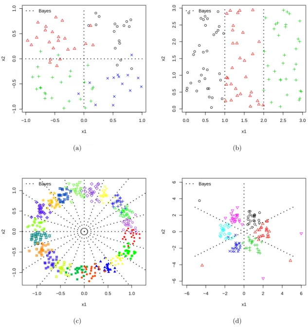
Example 1: In this example, we generate the data as follows. For the positive class, the 1stand 2nd
co-ordinates followN[(2,0)T, I2]. For the negative class, the corresponding distribution isN[(0,2)T, I2].
The remainingp−2 covariates followi.i.d. N(0,1), where pis the dimensionality of x.
The training data have 100 observations. The tuning parameter λ is chosen using a grid search
method. Specifically, for each candidate λ value in {2−10,2−9,· · · ,239,240}, we fit the model with
PLR, and the misclassification error rate on a tuning data, whose observations are independent and
identically distributed with respect to the training observations, is calculated. The tuning data have
100 observations. We choose the λ value that corresponds to the minimal error rate. Next a test
set of size 104 is used to evaluate the performance of both classification accuracy and probability
estimation. We repeat the whole procedure 1000 times to calculate the average misclassification rate,
P(Y 6= ˆY), and probability estimation error, #(test set)1 P
i∈test set(|ˆpi −ptruei |). We report average
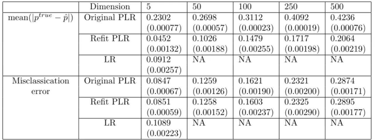
probability estimation errors and average misclassification rates in Table 2.1. The corresponding
standard errors are reported in parentheses. As a comparison, the regular logistic regression is also
used here.
We can see from Table 2.1 that the absolute difference betweenptrueand ˆpfor the refit method is
much smaller than the original estimator. This demonstrates the effectiveness of our refit method. In
terms of classification errors, the refit method is almost identical to the original fit. As an illustration,
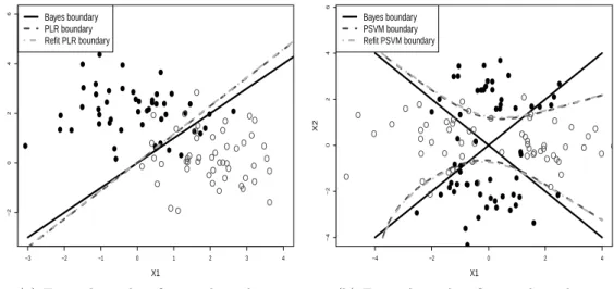
we plot the classification boundaries before and after the refit step, along with the Bayes boundary,
on the left panel of Figure 2.1, for one typical simulation. We can see that the refit step does not
change the boundary much.
Example 2: This is a nonlinear example. Similar to Example 1, only the first two covariates are
distributions as 12N[(2,0)T, I2] + 12N[(−2,0)T, I2], and the negative class is from a different mixture
of normal distributions as 12N[(0,2)T, I2] +12N[(0,−2)T, I2]. We use the PSVM as the loss function.
For efficiency in computation, we add the second and third order of the 1st and 2nd coordinates into
the original data, and then treat it as a linear learning. The training sample size is set to be 120.
We generate 120 tuning observations in a similar manner as in Example 1. The tuning parameter λ
is chosen in the same way as in the previous example, and the number of replications is also 1000.
We report the probability estimation errors and the misclassification rates in Table 2.2. The Bayes
boundary, the classification boundaries before and after the refit step are reported on the right panel
of Figure 2.1. In this example, a similar conclusion as in Example 1 can be drawn from the results in
Table 2.2 and the right panel of Figure 2.1.
Dimension 5 50 100 250 500
mean(|ptrue−p|)ˆ Original PLR 0.2302 0.2698 0.3112 0.4092 0.4236
(0.00077) (0.00057) (0.00023) (0.00019) (0.00076)
Refit PLR 0.0452 0.1026 0.1479 0.1717 0.2064
(0.00132) (0.00188) (0.00255) (0.00198) (0.00219)
LR 0.0912 NA NA NA NA
(0.00257)
Misclassication Original PLR 0.0847 0.1259 0.1621 0.2321 0.2874
error (0.00067) (0.00126) (0.00190) (0.00200) (0.00171)
Refit PLR 0.0851 0.1258 0.1603 0.2325 0.2895
(0.00059) (0.00152) (0.00237) (0.00290) (0.00177)
LR 0.1089 NA NA NA NA
(0.00223)
Table 2.1: The average classification and probability estimation errors using PLR for Example 1 with n = 100. The corresponding standard errors are reported in parentheses. The LR cannot be calculated for p≥50, and we use NA for those entries.
Dimension 5 50 100 250 500
mean(|ptrue−p|)ˆ Original PSVM 0.1892 0.2011 0.2473 0.3019 0.3698
(0.00030) (0.00019) (0.00024) (0.00054) (0.00033)
Refit PSVM 0.0801 0.1195 0.1278 0.1503 0.1610
(0.00377) (0.00560) (0.00573) (0.00399) (0.00298)
Misclassication Original PSVM 0.1621 0.1939 0.1944 0.1957 0.2016
error (0.00199) (0.00356) (0.00511) (0.00299) (0.00318)
Refit PSVM 0.1622 0.1940 0.1945 0.1952 0.2012
(0.00342) (0.00406) (0.00531) (0.00290) (0.00382)
Table 2.2: The average classification and probability estimation errors using PSVM for Example 2 with n= 120. The corresponding standard errors are reported in parentheses.
−3 −2 −1 0 1 2 3 4
−2
0
2
4
6
X1
X2
Bayes boundary PLR boundary Refit PLR boundary
(a) Example 1, classification boundaries
−4 −2 0 2 4
−4
−2
0
2
4
6
X1
X2
Bayes boundary PSVM boundary Refit PSVM boundary
(b) Example 2, classification boundaries
Figure 2.1: The left panel shows the classification boundaries of the original and the refit methods for PLR in Example 1. The right panel shows the classification boundaries of the original and the refit methods for PSVM in Example 2. Clearly the classification boundaries of the original and the refit methods are almost identical.
2.5 Real data
In this section we investigate the performance of our proposed refit method on two real data sets,
namely Liver and Ionosphere. The Liver dataset contains 345 patients with the class label being the
liver disorder status. There are 6 input variables related to blood tests and they are thought to be
sensitive to liver disorders that might arise from excessive alcohol consumption. For the Ionosphere
data, the goal is to clarify good versus bad radar returns using 34 input attributes. Good radar returns
are those showing evidence of certain structure in the ionosphere, and bad returns are those that do
not. There are 351 samples in total. More information about these datasets can be found on the UCI
machine learning repository database website, http://www.ics.uci.edu/~mlearn/MLRepository.
html.
In each example we randomly choose 70 observations for training, 75 for tuning, and the remaining
for testing. In each random split, λis chosen by a grid search as in the simulated examples, and we
compare the probability estimation of the original methods with that of the refit methods. We apply
PLR for both datasets. Since the underlying probability distribution is unknown, we evaluate the
CRE(ˆp) =−#(test set)1 P
test set{ 1
2(1 +yi) log [ˆp(xi)] + 1
2(1−yi) log [1−p(xi)]}. For each data set, weˆ
standardize the input covariates before the analysis. For the Liver data, the Gaussian kernel is applied,
and the kernel parameter σ is set to be the first quartile pairwise distance between the positive and
negative classes. Through 1000 times of random splitting, the CRE’s of the original estimator and
of the refit method are 1.959(0.001) and 1.908(0.004), respectively. For the Ionosphere data, linear
learning is used. The CRE’s of the original estimator and of the refit method are 3.211(0.062) and
0.525(0.006), respectively. This suggests that the refit method improves probability estimation for
both real data examples. Interestingly, the improvement for the Ionosphere data appears to be larger
than the Liver data, possibly due to its higher dimension of covariates.
2.6 Possible Future Work
In this chapter we investigate the problem of probability estimation for large margin classifiers and
illustrate the bias problem on class probability estimation created by shrinkage. We show that such
bias can be large for finite sample problems. As a result, alternative procedures are needed. Our
simple refit method helps to correct the scale problem introduced by shrinkage and yields accurate
class probability estimation.
As a remark, we would like to mention that the work of Zhu and Hastie [2003] provides a promising
path for further improvement of probability estimation. In particular, they proposed an interesting
idea of feature selection through density estimation. For our case, suitable feature selection via density
estimation may help to yield a more flexible and robust projection space for the refit step.
Our focus in this chapter is on binary classification. For multicategory problems, we believe similar
phenomena exist and corrections are necessary as well. Since there will be multiple classification
functions, the projection step is more complicated. Further investigation will be pursued.
2.7 Proofs
Proof of Theorem 2.2.1. Notice that minE{`[Y f(X)]}= minE{E
`[Y f(X)]|X =x}. Letting
S =E{`[Y f(X)]|X =x}=p(x)`[f(x)]+[1−p(x)]`[−f(x)], we have ∂S∂f|f=f∗ =`0(f∗)p−`0(−f∗)(1−
p) = 0. As `0(u) +`0(−u)<0,∀u, p(x) = `0[f∗(x)]+``0[−f∗0(x)][−f∗(x)]. Now taking the derivative ofp(x) with
respect to f∗(x) yields dfdp∗ =−
`0(f∗)`00(−f∗)+`0(−f∗)`00(f∗)
[`0(f∗)+`0(−f∗)]2 . Thus by Condition B.3, p(x) is a strictly
increasing function of f∗(x), which guarantees a one-to-one correspondence between them.
Proof of Theorem 2.3.1. Letx∗i =xTi β∗. Recall that ˆx∗i =xTi β. The empirical loss function weˆ
minimize in the refit step is
min γ0,γ1
1 n
n X
i=1
`[yi(ˆx∗iγ1+γ0)],
and we define
L(ˆγ0,ˆγ1) := 1 n
n X
i=1
`[yi(ˆx∗iγˆ1+ ˆγ0)].
Assume that ˆγ0 does not converge to 0 in probability, asn→ ∞. We then have a subsequence of ˆγ0’s
that converges to another real number z 6= 0 in probability. For simplicity, assume that the entire
sequence ˆγ0 converges to z. Note that as n→ ∞,L(0,1θ) converges toE[`(yx∗)] by Assumption C.3.
Because L(ˆγ0,γˆ1) does not converge toE[`(yx∗)] for any choice of ˆγ1 if ˆγ0→z, we can conclude that
for large enough n,L(ˆγ0,ˆγ1)> L(0,1θ), by AssumptionC.2. This contradicts the fact that (ˆγ0,ˆγ1) is
the minimizer of L. Thus ˆγ0 converges to 0 in probability, as n→ ∞. A similar argument can show
that ˆγ1 converges to 1θ in probability, asn→ ∞. This completes the proof.
Proof of Corollary 2.3.1. In weighted learning, the empirical loss function we minimize in the refit
step is
min γ0,γ1
1 n
n X
i=1
W(yi)`[yi(ˆx∗iγ1+γ0)],
and now the definition of Lbecomes
L(ˆγ0,γˆ1) := 1 n
n X
i=1
W(yi)`[yi(ˆx∗iˆγ1+ ˆγ0)].
The rest of the proof follows the same line as that of Theorem 2.3.1, except that L(0,1θ) converges to
CHAPTER 3: MULTICATEGORY LUM
3.1 Introduction
Classification problems are commonly seen in practice. When one faces a classification task, there
are many possible techniques to choose from. To list a few, logistic regression and Fisher linear
discriminant analysis (LDA) are very classical classification methods. The Support Vector Machine
[SVM, Cortes and Vapnik, 1995; Wahba, 1999] and Boosting [Freund and Schapire, 1997] are more
recent machine learning based large margin classification tools. Despite some known properties of
these methods, a practitioner often needs to face one natural question: which method should one
choose to solve the classification problem in hand?
Wahba [2002] discussed the concept of soft versus hard classification. Recall the difference between
soft and hard classifiers from Chapter 1. Typical examples of soft classifiers include logistic regression
and LDA. On the other hand, the SVM is a typical example of hard classifiers, which is without any
strong distributional assumption. Another example of hard classifiers is theψ−learning [Shen, Tseng
and Zhang, 2003]. When class probability estimation is necessary, one can perform multiple weighted
learning for probability estimation [Wang, Shen and Liu, 2008]. For a given problem, the choice
between hard and soft classifiers can be difficult. Recently, Liu, Zhang and Wu [2011] proposed the
LUM family, which is a rich group of classifiers in the sense that it connects hard and soft classifiers
in one spectrum. The LUM family provides a natural platform for comparisons between soft and hard
classifiers. More importantly, it enables us to observe the performance transition from soft to hard
classification.
The existing development on the LUM is limited to the binary case. For multicategory problems,
further development is necessary. In particular, probability estimation becomes more challenging as
one needs to estimate a probability vector. Furthermore, multicategory consistency is much more
involved, especially for hard classifiers. For instance, there are a lot of developments on multicategory
SVMs in the literature [Vapnik, 1998; Weston and Watkins, 1999; Crammer et al., 2001; Lee, Lin and
there is no dominating class, i.e, the maximum class probability is less than 0.5. So far, the only group
of consistent multicategory piecewise linear hinge loss functions available is the family of reinforced
hinge loss functions by Liu and Yuan [2011], which covers the loss by Lee, Lin and Wahba [2004]
as a special case. For probability estimation, there are several existing multicategory soft classifiers,
such as Adaboost in Boosting [Freund and Schapire, 1997; Zou, Zhu and Hastie, 2008b; Zhu et al.,
2009], logistic regression [Lin et al., 2000], proximal SVMs [Tang and Zhang, 2006], and multicategory
composite least squares classifiers [Park et al., 2010].
In this chapter, we propose new Multicategory Large-margin Unified Machines (MLUMs). Similar
to the binary case, the MLUM is a broad family that embraces many of the aforementioned classifiers
as special cases. It helps to shed some light on the choice between multicategory soft and hard
classifiers, and provides some insights on the behavior change from soft to hard classification methods.
Our theoretical studies show that the MLUM is always Fisher consistent, and is able to provide class
conditional probability estimation. Moreover, we extend the excess risk concept discussed in Bartlett,
Jordan and McAuliffe [2006] to the multicategory case and study its convergence rate. We also propose
an efficient tuning procedure for the MLUM family. Our numerical results show that the behaviors
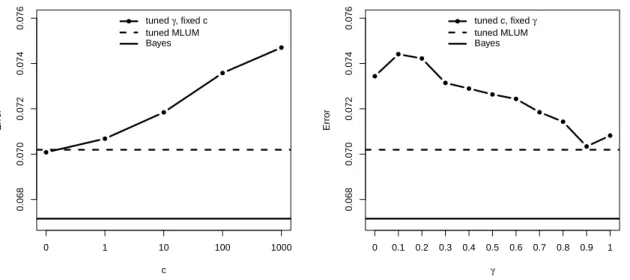
of different classifiers vary from setting to setting. In particular, we have the following observations.
Soft classifiers tend to give more accurate classification results by estimating the conditional
class probability when the true probability functions are relatively smooth.
Hard classifiers bypass the probability estimation and may work better when estimation of the
underlying probability functions is challenging, such as the step function.
When the data are noisy with outliers, soft classifiers tend to be very sensitive and unstable.
Some MLUM member in-between hard and soft tends to work the best. This was not observed
in the binary case [Liu, Zhang and Wu, 2011].
Although our observations may not hold for all classification problems, it can help us to understand the
classification behaviors better. Furthermore, our numerical results also suggest that the performance
of the proposed tuned MLUM is very competitive.
The rest of this chapter is organized as follows. In Section 3.2, we give some motivation and
introduce the MLUM family. Section 3.3 explores some statistical properties of the MLUM family.