Simulating Binary Inspirals in a Corotating Spherical Coordinate System

(1)

Simulating Binary Inspirals in a Corotating Spherical Coordinate

System

Travis Marshall Garrett

A dissertation submitted to the faculty of the University of North Carolina at Chapel Hill in partial fulfillment of the requirements for the degree of Doctor of

Philosophy in the Department of Physics and Astronomy

Chapel Hill 2007

(2)

Abstract

TRAVIS GARRETT: Simulating Binary Inspirals in a Corotating Spherical Coordinate System

(Under the direction of Charles Evans)

(3)

Dedication

(4)

LIST OF FIGURES

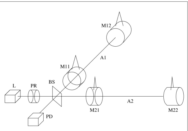
1.1 Interferometer Layout. L : Laser , PR: Power Recycler, BS: Beam Splitter, PD: Photo-Detector, M11-A1-M12: Mirror 1 and 2 on

arm A1, M21-A2-M22: Mirror 1 and 2 on arm A2 . . . 24 1.2 LIGO I and II frequency profiles (from [1]) . . . 25 1.3 LISA frequency profiles (from [1]) . . . 26 2.1 Diagram of the 1PN fields as generated by the main program (in

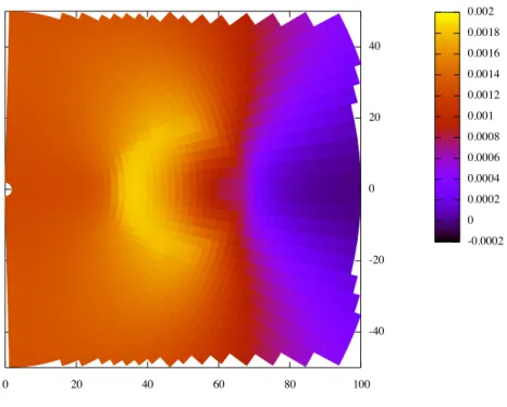
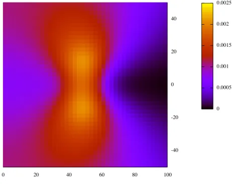
spherical coordinates). . . 45 2.2 Diagram of the 1PN fields given by directly integrating equation (2.31). . 46 2.3 Diagram of a binaries precession in both Nordstr¨om’s theory and

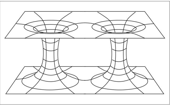
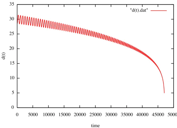
general relativity . . . 57 3.1 Kruskal-Szekeres mapping of a Schwarzschild Black Hole. . . 76 3.2 Wormholes connecting to the same second asymptotically flat universe. . 77 3.3 Wormholes connecting to different asymptotically flat universes. . . 77 4.1 Binary separation as a function of time. . . 113 4.2 Eccentricity e as a function of semimajor axis a for a numerical

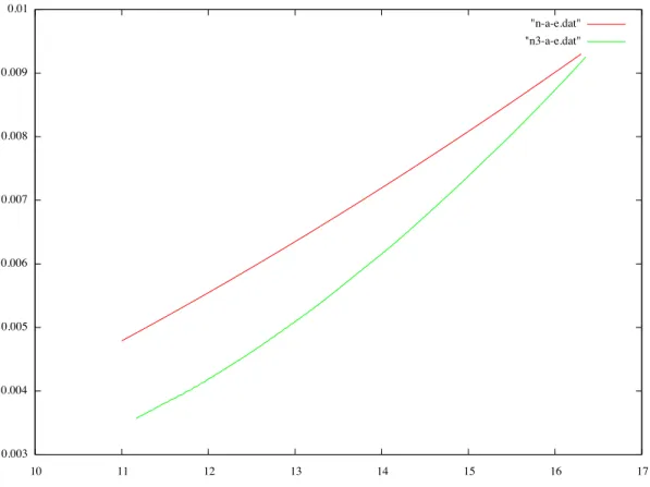
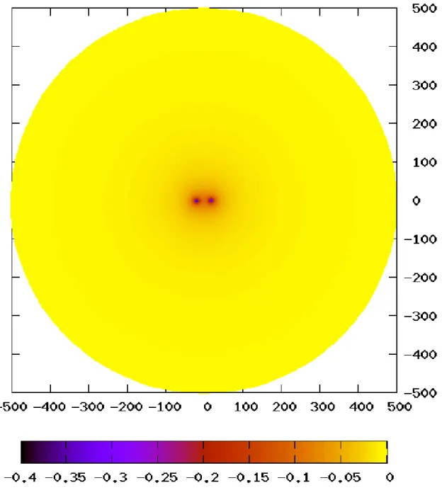
inspiral and a theoretical inspiral with the same Keplerian parameters. . 114 5.1 Equatorial slice of the field strength ϕ. The stars have radius

5M, are situated ±20M from the origin, and the outer boundary

is 500M from the origin. . . 131 5.2 Plotted is the log of the error e= sup|ϕN ewton/ϕ−1|against the

log of the number of radial grid pointsN. A linear fit gives a slope of−2.2±0.2, i.e. second order convergence. The lowest resolution grid usesN = 500 radial grid-points andLandM values up to 25. This is then doubled four times up to resolution with N = 8000

radial grid points and L and M values up to 400. . . 132 5.3 Plotted is the error = (ar)/(1/d2)−1 of the radial acceleration

(compared to the expected Newtonian inverse square law) as a function of the separationd. Standard second order accurate finite differencing methods are used to find the derivatives of the field en route to calculating ar. The error grows to 25 percent for a

separation of 60M, despite the field being correctly resolved to

(8)

5.4 Another plot of the error = (ar)/(1/d2)−1 of the radial

acceler-ation, but now using 12th order finite differencing to extract the derivatives. The result is now accurate to with 0.3 percent, which

is the same accuracy the field is resolved to. . . 135

5.5 Plot of ϕN ewton/ϕ for a separation of 14M. The waves differ from the Newtonian field by about 5 percent. . . 137

5.6 Plot of the acceleration in the φ direction as a function of sep-aration. The fit value of 1.466 agrees with the theoretical value 29/2/15 to within 3 percent. . . 138

5.7 Separation as a function of time for a quasi-circular inspiral. . . 139

5.8 Plot of the rate of energy loss of the binary dE/dt as a function of the separation d, compared to the theoretical value. . . 140

5.9 Plot field ϕ(t, r =Rmax, θ = π/2, φ = 0) at the outer boundary as a function of time, showing the chirp waveform. . . 141

5.10 Eccentric inspiral: separation as a function of time. . . 144

6.1 Plot of conserved density as a function of radius ρ∗(r) for three stars with polytropic equations of state Γ = 4/3, 5/3, and 2. All stars are constructed to give Mgrav/R= 1/5. . . 149

6.2 Total gravitational and rest masses as a function of the outer radius for a range of stars with polytropic equation of state Γ = 4/3. . . 152

6.3 Total gravitational and rest masses as a function of the outer radius for a range of stars with polytropic equation of state Γ = 5/3. . . 153

6.4 Total gravitational and rest masses as a function of the outer radius for a range of stars with polytropic equation of state Γ = 2. . . 154

6.5 Equatorial slice of the source density . . . 160

6.6 Source errors after convolution. . . 161

6.7 Equatorial slice of the field ϕ . . . 165

6.8 Top down view of the equatorial slice of the field ϕ . . . 166

6.9 Side view of the equatorial slice of the field ϕ . . . 167

6.10 Side view of ϕ/ϕan . . . 168

6.11 Side view of ϕ/ϕan at double resolution . . . 169

(9)

6.15 Molecular diagram for the Crank-Nicholson implicit finite differ-encing scheme. Spatial derivatives are taken and averaged at the

N and N + 1 time steps. . . 174 6.16 Molecular diagram for the modified, second order in time

Crank-Nicholson differencing scheme. Spatial derivatives are taken and

averaged at the N −1 andN + 1 time steps. . . 175 6.17 1/(1 +x2_{) and a regular spacing interpolation.} _{. . . .} ₁₈₂

(10)

Chapter 1

(11)

1.1 A New Window

Over 90 years have passed since Einstein’s original 1916 prediction of gravitational waves [2] [3], and they still have not been directly observed. We will very likely observe them before the 100th anniversary however, thanks to the efforts of an international team of scientists dedicated to detecting these subtle ripples in the fabric of spacetime. The first detection will inaugurate a new field of science and open a new window onto our universe.

The long wait between the prediction and detection of gravitational waves is a reflection of the difficulty of the task. Gravitational waves are very hard to produce: giant, dense concentrations of matter need to be accelerated to very high speeds in order to generate waves of a nontrivial magnitude. Only violent astrophysical systems such as colliding black holes and neutron stars and supernova explosions are powerful enough to generate waves that we could detect. Gravitational wave observation will thus allow us to explore much more deeply into the hearts of these exotic environments, and test some of general relativity’s most extreme predictions.

(12)

of the data generated by the interferometers, it is crucial to generate a database of theoretical waveforms. These waveforms will also allow us to compare the detected waves produced by strongly gravitating systems to the predictions of general relativity. The goal of this thesis is to develop numerical methods that give more accurate theoretical profiles of the gravitational waves produced by a pair of compact bodies spiraling into each other. The core of our method is to use a corotating spherical reference frame to model the crucial late inspiral of a compact binary system. We develop our methods by modeling binary inspirals in Nordstr¨om’s scalar theory of gravity. We find that our code produces long stable evolutions that match the analytic inspirals that we have calculated for this theory.

In the rest of the introduction we will give an overview of gravitational wave science. We will discuss the physics of gravitational waves, and then examine likely astrophysical sources of gravitational waves, which we hope to detect. This is followed with an overview of the laser interferometers. The next two chapters describe post-Newtonian calculations and numerical relativity. We will primarily develop methods for numerical relativity, and check our results with post-Newtonian analysis. Chapters four and five are the current drafts of our two papers, which contain, respectively, our work on semi-analytic calculations of binary orbit decay in Nordstr¨om’s theory, and our numerical simulations of this process. The sixth chapter describes the details of the numerical implementation of our methods, and we finish with conclusions.

1.2 Nordstr¨

om’s 2nd Theory

(13)

If the matter source ρ begins to accelerate then the Newtonian potential Φ instantly responds at all points in space. If true, this would allow for signals to be sent faster than the speed of light, and thus cause a breakdown of causality (although see [4] for an interesting discussion).

A simple solution is suggested by the transition from electrostatics to electro-dynamics: let the Laplacian operator change to the d’Alembertian wave operator:

∇2_Φ _→ _{Φ. In this case an accelerating source would generate waves that spread}

out at the speed of light, restoring causality. Additional modifications could then be sought so that the new theory has both relativistic force laws and matches Newton’s theory in the appropriate limit. This was the path taken by Gunnar Nordstr¨om in 1913 during the development of his 2nd theory of gravitation. Einstein was impressed with the theory, and he and Fokker showed that by using a conformally flat metric gµν =ψ2ηµν that the main equations could be written in a geometric form:

R= 24πT (1.2)

i.e. the Ricci scalar is equal to the trace of the stress energy tensor. Later Weyl introduced the Weyl curvature tensor Cαβγδ which measures how a metric deviates

from conformal flatness. Thus

Cαβγδ = 0. (1.3)

can be combined with (1.2) to completely describe the theory.

(14)

1.3 Gravitational Waves

Einstein took a somewhat different path in his search for a relativistic theory of gravitation. Instead of explicitly searching for a wave-like version of Newtonian gravity, Einstein was guided by two theoretical principles towards his famous theory (see e.g. [5]). The first is the principle of equivalence: the acceleration of a body in a gravitational field is independent of the bodies’ internal structure. The second is Mach’s principle: the structure of spacetime should be influenced by the distribution of matter in it. Einstein used these principles – along with the mathematics of curved manifolds as developed by Riemann, the fact that small local volumes of spacetime should be approximately Lorentzian, and the necessity to match Newtonian gravitation for weak fields – to develop general relativity. In general relativity it is the curvature of spacetime that generates gravitational effects. The curvature is in turn generated by the distribution of mass-energy throughout spacetime as described by the Einstein equations:

Gµν = 8πTµν (1.4)

While not explicitly founded on the idea of gravitational waves like Nordstr¨om’s theory, it quickly turned out that general relativity also includes them (although the physicality of the waves was debated for decades - see [6], [7], and for general references on gravity waves see [8], [9], [10]). In order to demonstrate that general relativity contains Newtonian gravitation as a weak field limit, one splits the physical metric gµν up into a flat background metric ηµν and a small perturbation hµν (with

|h|<<1 and thus ignoring higher order corrections):

(15)

also allows us to investigate gravitational waves (see e.g. [11]). We take equation (1.5) and plug it into the Einstein equation (1.4), and discard terms of order|h|2 _and

higher to get:

∂γ∂µhνγ+∂γ∂νhµγ −∂γ∂γhµν−∂µ∂νh (1.6)

−ηµν(∂γ∂δhγδ−∂γ∂γh) = 16πTµν

where the background metric is used to raise indices: ∂µ ₌_ηµγ_∂

γ, h =ηγδhγδ. This

equation can be simplified by defining:

¯

hµν =hµν−

1

2ηµνh (1.7)

which reduces (1.6) to:

∂γ∂µh¯νγ+∂γ∂νh¯µγ −ηµν∂γ∂δhγδ (1.8)

−∂γ∂γ¯hµν = 16πTµν

This is still somewhat complicated but one can show that by choosing an appropriate infinitesimal coordinate transformation (xµ0 ₌_xµ₊µ_{) that the following gauge choice}

is possible:

∂γ¯hµγ = 0 (1.9)

This is similar to the Lorentz gauge choice ∂γAγ = 0 used in electrodynamics. This

thus reduces (1.8) to:

∂γ∂γ¯hµν =−16πTµν (1.10)

which includes the vacuum case:

¯hµν = 0 (1.11)

(16)

accelerates waves will propagate out at the speed of light and inform the rest of spacetime.

1.3.1 Weak Gravitational Waves

We will next investigate the properties of the waves given by (1.11). In order to do so consider bodies that are initially both at rest in a local Lorentz reference frame. Position body A at the origin, and bodyB at a positionξ. We thus want to see how bodyB moves with respect toA in response to a gravitational wave moving through their volume. To do so we use the equation of geodesic deviation:

uγ∇γ(uδ∇δξj) =−R j αµβu

α

uβξµ (1.12)

To lowest order the 4-velocities of the bodies are u0 _{= 1 and} _ui _{= 0, and we can}

also set up the position of body B as its initial position plus a small time dependent perturbation: ξ=ξ0+δξ(t). Thus equation (1.12) simplifies to:

∂_t2δξj =−Rj₀_k₀ξ₀k (1.13)

In the previous section we made use of the Lorentz-type gauge condition (1.9) to reduce the equation of motion for the metric perturbation to a wave equation (1.11). We have additional gauge freedom since a further transformation of the type ∂γ∂γµ= 0 won’t change the validity of (1.9). We can use this to transform the metric

perturbation into Transverse-Traceless form hT T

µν, which is related to the Riemann

tensor via:

Rj0k0 =−

1 2∂

2

th T T

(17)

motion as the gravitational wave passes is:

δξj = 1 2h

T T jk ξ

k

0 (1.15)

We note from (1.15) that the amount by which the test body B’s position is perturbed (from the vantage point of A) is proportional both to the total separa-tion between A and B and the magnitude of the gravitational wave. This will be important later for the functioning of the interferometers. Furthermore the metric perturbationhT T

µν only distorts spatial distances that are perpendicular to its direction

of propagation (transverse), and its trace is zero (traceless) (this is due to the wave equation and gauge choices we have made).

Let the test bodiesAand B be oriented in thex-y plane, and let the gravitational wave propagate along thez axis. The only nonzero components arehT T_xx =−hT T_yy and hT T_xy = hT T_yx, so we have two degrees of freedom, corresponding to two polarizations. Designate the two polarizations by the amplitudes of the waves: h+ = |hT Txx| and

h× = |hT Txy |. Consider a h+ polarized wave passing by the test bodies at a point in

time. With the phase of the wave currently equal to zero, the x component of the distance will be larger by:

δξx = 1 2h+ξ

x

0 (1.16)

and they component will be smaller:

δξy =−1

2h+ξ

y

0 (1.17)

In general a circle of test particles arranged around A will form an oscillating ring, while a h× polarized wave will form a similar oscillating ring only rotated by 45

degrees. It is also possible to combine the h+ and h× polarizations to form right

(18)

waves. For instance, consider the waves emitted by a standard binary in quasi-circular orbit. In the plane of the binary the waves will be purely h+ polarized, while the

waves emitted in the polar directions will be purely circularly polarized, with a smooth transition for intermediate angles.

Note also that these two polarizations are the simplest solutions to the vacuum case of equation (1.11):

hT T_xx =−hT T_yy =_R{h+e−iω(t−z)} (1.18)

and

hT T_xy =hT T_yx =_R{h×e−iω(t−z)} (1.19)

A general solution can be formed from a superposition of these monochromatic waves. If we consider a rotation of our coordinate system about the z axis through the angle θ we find that the waves in the new coordinates are related to the old by: h0₊ =h+cos(2θ) +h×sin(2θ) andh0×=−h+sin(2θ) +h×cos(2θ). Thus a rotation of

180 degrees gives waves symmetric to the original. This is why quantized gravitational waves would be spin 2 particles, as a spinswave requires a rotation through an angle of 360/s degrees to return it to its original orientation.

1.3.2 Gravitational Waves Traveling Through the Universe

(19)

perhaps gradually focusing or diverging. Much the same for gravitational waves as they travel from their sources to the solar system.

To make this idea more concrete we can take the overall Riemann tensor which describes the overall gravitational state in the universe, and split it into a curved background and the waves which propagate over it. First take the average of the Riemann tensor, integrating over a distance much longer than the wavelengths of the waves: |Rαβδγ|. This gives the curvature of the background gravitational fields. The

gravitational wave Riemann tensor R(_αβδγGW) is then the difference between the overall Riemann tensor and its average:

R_αβδγ(GW) =Rαβδγ− |Rαβδγ| (1.20)

This is a valid procedure in our universe, where the curvature of the waves h/λ2 ∼

10−22/(109cm)2 is much greater than the curvature of the universe: ∼1/1056cm2. The wave equation then also needs to include covariant derivatives that are with respect only to the background curvature (as signified with a | instead of ;):

¯

hµν|γγ = 0 (1.21)

Higher order terms are also needed for completeness, although they are usually very small for realistic situations and can be dropped. The waves can thus be considered perturbations about the background curvature.

Suppose that the waves have traveled far enough from their source to be approxi-mately planar. This then allows for the eikonal or geometric optics approximation to be made. Using the previous arguments the wave can be put in the form:

(20)

whereφ=ω(z−t),φ|µ=kµ, andhαβ|β →Aαβkβ = 0, that is the waves are transverse,

the propagation vector is null kβkβ = 0 and the waves are parallel propagated along

null geodesics Aαβ|µkµ = 0. Since the waves propagate along null geodesics of the

background curvature, they can undergo gravitational lensing and redshifting, in the same way as electromagnetic waves do.

1.3.3 Generation of Weak Gravitational Waves

We will now consider the generation of gravitational waves by sources that have negligible self gravity. The negligible self gravity stipulation allows us to use equation (1.10), as the first order perturbative expansion will not be sufficient for sources with appreciable self gravity. It turns out, as we will see later, that sources with strong gravitational self fields give rise to similar waves. The Green’s function solution to (1.10) is:

¯

hµν(t, x) = 4

Z _T

µν(t− |x−x0|, x0)

|x−x0_| d

3_x0 _(1.23)

This will generally not be in the transverse traceless gauge, but it can be subsequently cast into it by only keeping the components of h perpendicular to the direction of propagation and subtracting off the trace.

Several more assumptions are made to reduce this to a useful expression. Generally we are interested in the waves far from their source, and thus the|x−x0|term in the denominator of (4.46) can be approximated byr, the distance from the measurement point to the center of the wave source, and shifted outside the integral. We can furthermore show that Tjk _{can be transformed (by using integration by parts and}

Tµν

,ν = 0) into T00,00xjxk, which transforms (4.46) to:

hT T =

4 ∂2

Z

T00xj0xk0d3x0

T T

(21)

moment of the mass-energy T00 (to leading order).

When it is necessary to include sources with appreciable self-gravity (as will usu-ally be the case), then it will be useful to construct a pseudotensor τµν such that (Tµν₊_τµν₎

,ν = 0 [12]. This allows us to construct:

¯

hµν(t, x) = 4

Z

(Tµν+τµν)ret

|x−x0_| d

3_x0

(1.25)

and we can proceed as before, under suitable restrictive assumptions. This procedure will be considered in more detail in the post-Newtonian methods chapter.

1.4 Astrophysical Sources

With the general characteristics of gravitational waves now in hand, we next con-sider the possible astrophysical sources that we may hear with the new observatories (note that we will often use ”hear” in place of ”detect” as in many ways gravitational waves are analogous to sound waves, thus complementing the electromagnetic light that we see – see e.g. [13], and for more source overviews see [1] and [14]). There is a wide variety of possible sources, but the most likely to be initially detected are pairs of compact bodies in tightly bound orbits, so we will focus in this section on these objects. Rapidly evolving Neutron Star (NS) and Black Hole (BH) binaries are the most likely candidates to be heard first by the ground based detectors and slowly evolving White Dwarf (WD) binaries are all but guaranteed to be detected by a space based detector (see [15] for detailed descriptions of these objects). These binaries have very small separations and have orbital velocities that are a substantial percentage of the speed of light, and are thus producing copious gravitational waves. The energy and angular momentum carried away by the waves causes the binary system to decay until the compact bodies merge in a final burst of gravitational radiation.

(22)

to do a careful analysis to see if it is reasonable to expect that we will hear any waves from these systems during the lifetime of operation of the detectors. We thus need to combine astronomical observations and theoretical considerations to form models that describe how galaxies are populated with different types of star systems.

1.4.1 Stellar Populations

To begin the description we zoom all the way out to the beginning of the universe. Several hundred thousand years after the big bang the universe had cooled sufficiently for the protons and electrons to combine and form a neutral hydrogen gas, thus releasing the photons that had previously been trapped within the plasma. These photons have traveled freely since then, and have now appear to us as microwave radiation, having since been redshifted by about a factor of thousand. This gives us the Cosmic Microwave Background (CMB), as originally discovered by Penzias and Wilson [16], [17].

Recent geometric investigations of the slight inhomogeneities in the CMB show that the universe is very nearly flat and thus the average density of the universe is very close to the critical value of ρcrit = 1.17×1011M/M pc3. The inhomogeneities were

at level of one part in 105_{during the formation of CMB, and went on to seed the birth}

(23)

We then need to estimate the fraction of these stars that are the compact bodies we are interested in. First we need to know the rate at which stars of different masses are produced. The current overall Star Formation Rate (SFR) is estimated to be about one solar mass star per year in a 100 cubic Megaparsec volume [18]:

SF R= 0.013+0₋₀._.007₀₀₅ M

yrM pc3 (1.27)

(note that this is averaged over large enough volumes such the universe is homo-geneous). The current SFR is lower now than it has been in the past. Since star formation began after the big bang it has been decreasing in rate roughly exponen-tially:

SF R∝e−t/τ (1.28)

where τ = 6 Gyr [19].

With the rate star formation in hand, we now need to know the Initial Mass Function, which gives the fraction of stars formed at a particular mass [20], [21]. Fitting to observational data gives the fraction of stars ξ(m) within dm of mass m as:

ξ(m)dm= SF R(Myr

−1₎

0.92M2

×(M/0.5M)−1.3 (1.29)

for M <0.5M and

ξ(m)dm= SF R(Myr

−1₎

0.92M2

×(M/0.5M)−2.3 (1.30)

for M >0.5M. Thus most stars produced are less massive than the sun.

(24)

mass M is approximately:

L'L

M M

3.5

(1.31)

This reflects that stars more massive than the sun consume their fuel at a much more rapid rate. In a hot dense plasma only nucleons in the upper tail of the thermodynamic distribution will have sufficient kinetic energy to overcome the electrostatic potential and fuse. The fusion rate is increased by quantum tunneling, which is exponentially suppressed by the magnitude of the potential barrier being tunneled through. These effects combine to give the steepness in equation (1.31). The rapidity of burning determines an approximate life span TM S for main sequence stars as a function of

their mass:

TM S '13×109

M M

−2.5

yr (1.32)

Among all the stars that have been born since the big bang, those less massive than the sun are almost all still on the main sequence, while most of those more than about 2M have completed their life cycle and are now either a WD, NS, or BH. We

can thus compute that out of the density of stars in the universe (1.26), about 76 percent are luminous main sequence stars, and the rest are compact remnants, with about 18 percent white dwarfs, 2 percent in neutron stars, and the final 3 percent in black holes.

1.4.2 Stellar Evolution

As a main sequence star with mass M _& M ages it burns through the supply

(25)

of an astronomical unit. This is the red giant phase of a star, with examples ranging from the approximately solar mass Arcturus to the∼15MAntares. This late phase

of the star’s evolution will turn out to be very important later, as it can lead to mass transfer in a binary star system, and a corresponding decrease in the binary separation.

The final fate of the star as it evolves through the red giant stage depends on the mass of the star. For stars less than about 2.5M the helium in the core is held up

mainly by degeneracy pressure. Thus as the star burns more hydrogen in the outer shell, and the temperature rises to 3×108K, the helium can burn explosively in a process known as the helium flash (which generally does not release enough energy to blow apart the star). In heavier stars the helium core is supported by thermal pressure and begins burning more smoothly. As the helium burning in the center finishes, leaving behind carbon and oxygen, and begins to burn helium in outer shells the star enters the Asymptotic Giant Branch (AGB). Stars less than about 8M

will not go on to burn the carbon and oxygen in their cores, and instead blow off a large percentage of their mass, producing a planetary nebula and leaving behind a carbon-oxygen WD. For stars that are between 8M and 10M the carbon-oxygen

core can detonate in a manner similar to the helium flash, but it is not clear at this time whether this will blow the star apart or not.

For stars greater than about 10Mthe carbon-oxygen core will burn non-explosively,

(26)

star. Neutrinos carry away most of the gravitational potential energy, and a small percentage of these interact with the rest of the star, blowing it apart in a type II supernova. A classic example is supernova SN1054, which left the Crab Nebula and a pulsar behind. A problem with supernovae, in terms of producing binary NS systems, is that the supernova explosion generally ejects the new neutron star at considerable speed. This is due to asymmetry in the collapse process, as an asymmetry of 1 per-cent would be sufficient to explain the neutron star kicks that are observed. This will generally disrupt a binary system, and perhaps only one in a hundred neutron stars will remain in a binary system after a supernova.

If the star is massive enough, around M > 25M then the core collapse is too

massive to be halted by the formation of a neutron star, and it collapses directly into a black hole. A massive accretion disk can then form around the new black hole, producing polar jets that punch through the star. These are hypernovae, and are leading candidates as the causes of long duration Gamma Ray Bursts (GRBs).

These processes give us compact bodies that can produce loud gravitational waves, but they furthermore need to be produced in tight binary orbits, with separations on the order of a light second, so that gravitational radiation can then cause them to spiral in and merge within the age of the universe. Binary star systems are very common, accounting for perhaps half of all the stars in a galaxy. Their Keplerian parameters are log-normal distributed, so that binary systems with separations of one AU and 10 AU have the same probability of being formed.

(27)

giant star having formerly been the most massive, but then having transferred much of its mass to its companion upon expansion. Another famous example is Cygnus X-1 [25] [26], where an O-B supergiant is feeding the accretion disk of its black hole companion, and producing bright X-rays. Supernova explosions are another possible result of accretion processes: if a white dwarf accretes enough matter from a red giant companion to reach the Chandrasekhar mass, it will usually detonate the carbon and oxygen in a type Ia supernova, as in supernova SN1572 [27].

The transfer of material from one star in a binary to the other via the Roche lobe can also cause the binary stars to spiral into each other. For instance it is thought that AM CVn binaries (see e.g. [28], [29],[30]) are the product of several cycles of accretion and inspirals, resulting in a tight enough orbit to emit gravitational waves (GWs) observable by LISA. It is thus an important pathway to bring binaries close enough together so that gravitational radiation can then cause an inspiral and merger within the lifetime of the universe (generally NS-NS need to have separations on the order of the radius of the sun in order to spiral in quickly enough).

1.4.3 Expected Compact Binary Detection Rates

In order to estimate the number of sources that the interferometers can be ex-pected to hear, all of these factors can be combined in massive Monte Carlo simu-lations of millions of binary systems in order to see what percentage evolve into the tight compact binaries we need. For detection purposes we also need to consider the amplitude and the frequency of the waves produced. The amplitude is crucial as this determines the volume of space in which we would be able to detect the GW source. The frequency is likewise crucial as the detectors are only sensitive to GWs within a certain bandwidth. Compiling the theoretical models and observational data we find the following expected detection rates for NS-NS, NS-BH, and BH-BH binaries:

(28)

post-Newtonian calculations, we can show that the amount of time tmerge that

a binary has left before it merges can be related to the binary’s frequency and the rate of change of the frequency: tmerge ∝ f /f˙. We thus hear about the

last 3 minutes of a NS-NS inspiral in LIGO. We thus need to estimate the rate at which NS binaries are entering the final phase of their inspirals in the local region of the universe.

Neutron star binaries are the systems we have the best observational data for. In 1974 Hulse and Taylor discovered the pulsar in PSR1913+16 which was determined to be orbiting another neutron star (see e.g. [31]). The binary was tight enough that the orbital parameters could be observed to evolve over the years due to the emission of gravitational radiation, in precise agreement with the predictions of general relativity. PSR1913+16 has about 300 millions years until the stars merge and their waves enter the LIGO frequency band. Since this discovery several other binary pulsar systems have been located. Compiling the observational data, Phinney derived an expected NS-NS merger rate of 10−6 _per

year in the Milky Way [32], which subsequent studies have tended to reproduce. However the recent discoveries of new binary pulsar systems, including PSR J0737-3039 in which both neutron stars are pulsars and which has only 80 million years left until merger, somewhat increases the expected merger rate: [33], [34].

(29)

In addition to the binary pulsar systems that have been directly discovered, it is also suggested that short gamma ray bursts (GRB) may be due to the merger of binary neutron star systems: [35], [36], [37]. If true this information could affect the expected hit rate. However, alternative hypotheses are offered for the progenitors of short GRBs - for instance they may also originate from erupting magnetic fields on neutron stars: [38].

• NS-BH: Unlike binary NS systems there are currently no known NS-BH binaries in the Milky Way, (although there are examples of systems such as Cygnus X-1 that have the potential to evolve into one). It is possible however that some of the gamma ray bursts detected at large distances are due to NS-BH systems where the NS has grown close enough to the BH to be tidally disrupted, thus forming an accretion ring about the BH and generating relativistic polar jets. In general the uncertainty in merger rate is greater, and plausible estimates need to rely much more on population synthesis models. Initial LIGO will be able to see these systems out to about 40 Mpc, and the estimated detection rate is similar to that for NS-NS systems – somewhere from 0.001 to 1 events per year. As before, LIGO II will observe over a thousand times the volume, and the hit rate will go up accordingly.

• BH-BH: As with NS-BH binaries, there are no known∼10Mblack holes

bina-ries, and we need to use population synthesis studies to give expected formation rates. While these studies suggest that the rate of formation of these per galaxy is lower than NS-NS binaries, they can be heard out to about 100 Mpc with LIGO I, and thus are the most likely systems to be first detected, with event rates estimates ranging from 0.05 to 1 a year [39] .

(30)

Globular Clusters are old, dense groups of stars – sometimes 106 stars within a radius of 10 pc – that are found orbiting many galaxies including our own. Due to the density of stars, there is considerable interaction between the stars, and in general heavier objects like black holes will migrate towards the centers of the globular clusters, where further interactions can cause black hole binaries to form that are tight enough to merge within the lifetime of the universe. Statistical models of these systems indicate that observable mergers of these cluster black holes may occur at the same rate as those in the galactic field [39].

1.4.4 Other Gravitational Wave Sources

In addition to neutron star and black holes binaries (which are the first objects we expect ground based detectors to hear) there are other interesting possible systems that we may detect. We will likely have to wait for advanced LIGO or LISA (depend-ing on the frequencies in which they radiate) to hear them. For instance there are so many tight WD-WD binaries in the Milky Way that their waves will combine to form a region of noise within a section of LISA’s sensitive range (see e.g. [40]). We might also hear a neutron star - white dwarf binary like J141-6545 NS-WD which has a pulsar that is one million years old (indicating a reasonably high formation rate). Simulations of the evolutions of NS-WD systems like these can be found in [41]. On the other hand we can have extremely massive binaries: LISA may hear the gravi-tational waves produced by the inspiral of supermassive black hole binaries. These are expected to be quite rare, but we can essentially hear them across the visible universe. Successive mergers are also a possible formation pathway for the creation of these massive black holes (see e.g. [42]).

(31)

small ”mountains” in their crust are another possible detectable source. The very strong gravitational fields on the surface will act to flatten the mountains, but there are plausible scenarios where they could still be produced. For instance they could be created if the neutron star accretes material from a companion on a different axis than it is revolving on, or is heated nonuniformly. Low Mass X-ray Binaries (LMXB) give an example of this, and LIGO 2 will be able to adapt its sensitivity profile to search for the waves from these objects: [45], [46]. Another interesting possible source is the stochastic GW background created during the big bang – see [47] for instance. Perhaps the most exciting possibility is that we will discover waves from a new, surprising source, as has often happened in the past when we have opened new windows onto the universe.

1.5 Interferometers

The age of experimental gravitational wave science began with Weber and the construction of resonant bar detectors [48]. Centered around large rods of metal, these detectors are designed so that a passing gravitational wave of the right frequency will stimulate a harmonic vibration in the rod. Weber believed that he detected the presence of gravitational waves, although this was later attributed to noise. The best current resonant bar detectors have sensitivities of abouth∼4×10−19[49], although they are only sensitive in a small frequency band.

Modern GW detector design is based on interferometry (see [50], [51] for overviews). Weiss showed 1972 that it should be possible to construct a laser interferometer that is sensitive enough to detect the distortions in space-time due to a gravitational wave passing through the earth [52]. Later in the 70s Forward built the first prototypes [53], with sensitivities of about h ∼ 10−16_{. Research since then has resulted in the}

(32)

TAMA300 [57], which have sensitivities of about h ∼ 10−22, thus making the detec-tion of gravitadetec-tional waves plausible. Advanced LIGO [58] will increase the sensitivity to h∼ 10−23, which will then make detection quite likely. Plots of the sensitivity as a function of frequency for both LIGO I and LIGO II, along with the gravitational wave signatures of some standard sources, is given in figure (1.2) The space based detector LISA [59] is being planned which will operate at a lower frequency band than the ground based detectors, and is also quite likely to detect GWs. A plot of LISA’s sensitivity profile and some standard sources is given in figure (1.3).

A general schematic of a laser interferometer is given in figure (1.1). A laser beam is produced by the laser at (L) and passes through a Power Recycler (PR) to the Beam Splitter (BS), which splits the beam into two. These two beams then travel down orthogonal vacuum tube arms A1 and A2, reflect off of the mirrors M12 and M22 at ends of each, and are then recombined at the PhotoDetector (PD). The laser beams combine to form an interference pattern at (PD), and thus if a GW passes through the detector it will slightly change the arm lengths A1 and A2 and thus perturb the interference pattern. The trick is to then sufficiently reduce the noise in the detector so that perturbations in spacetime of the order h∼10−22 can be detected.

There many sources of noise in laser interferometers, but here we will only discuss a few of the primary ones. Ground based detectors are most sensitive to waves in the 50 to 500 Hz range. The main source of error in the higher frequency range is the inherent quantum fuzziness in the laser light, referred to as ”shot noise”, while sensitivity at lower frequencies is limited by vibrations in the earth.

1.5.1 Detector Reference Frames

(33)

interfer-PD BS

A1

A2

L PR

M11

M12

M21 M22

(34)

(35)

Figure 1.3: LISA frequency profiles (from [1])

that we will base our measurements in. In the Local Lorentz Frame (LLF) gauge the metric is equal to the flat space metric ηαβ plus corrections that are on order of the

Riemann tensor |Rµνδγ| times the square of the displacement from the originL. The

Riemann tensor in turn is proportional to the amplitude of the gravitational waves divided by the square of their wavelength. We thus find:

gαβ =ηαβ +O(|Rµνδγ|L2) = ηαβ+

L λ

2

h (1.33)

This forms a simple coordinate system to work in, as many of the subtleties of general relativity can be ignored. Note that the ground based detectors are not in Lorentz frames however, since they remain stationary with respect to the ground instead of being in free fall. We thus need to accelerate the LLF by g, giving us the Proper Reference Frame of the interferometer. An example metric would be:

(36)

for h+ polarized GWs propagating perpendicular to the surface of the earth.

Note also that the LLF gauge is only valid for distances less than the length of the gravitational wave: L < λ, as the approximation does not converge for larger distances. This is a valid approximation for LIGO where the gravity waves are several thousand kilometers long, but not for LISA. For LISA the calculations need to be done in the Transverse Traceless (TT) gauge, which converges globally for weak waves:

gαβ =ηαβ +hT Tαβ (1.35)

In the TT gauge the distance L does not change at lowest order – instead the laser beam is modified by the metric perturbation as it propagates, resulting in the same phase shift as the LLF gauge when it is valid.

1.5.2 The Shot Noise Limit

Choosing an appropriate reference frame, we re-derive equation (1.15), and find that the change ∆L in the lengthL of one of the interferometer arms is:

∆L∼hL (1.36)

The change in length of +∆L in one arm and −∆L in the other combine to give a total phase shift of

∆φ= 4πLh λe

(1.37)

at the photodetector (PD), where λe is the wavelength of the laser light used. In

(37)

back and forth several hundred times along the arms before being recombined to form the interference pattern. In figure (1.1) this is accomplished by constructing Fabry-Perot cavities between mirrorsM11 andM12 on arm A1 and likewise between mirrorsM21 andM22 on arm A2. With a number of bouncesB the total phase shift becomes:

∆φ= 4πBLh λe

(1.38)

The laser light used is in the visible spectrum, so the phase shift is about ∆φ ∼10−9_.

We thus need to see if it is possible to distinguish phase shifts of this magni-tude with a laser. We find that there is an upper bound to the accuracy given by quantum mechanical uncertainty relations. While not as simple to derive as the position-momentum uncertainty relation, one can generally show that the uncertainty in energy and time in a system follow ∆t∆E _& _~. The uncertainty in the measure-ment time is related to the uncertainty in the phase by ωe∆t = ∆φ, where ωe is the

frequency of the laser light.

The energy collected is equal to the energy of each photon ωe~ times the total

number collected Nγ where the collection time is half the period of the gravitational

wave TGW/2 = 1/(2f) with frequencies of about f ∼ 100 Hz. For a coherent light

source like a laser, the uncertainty in the number of photons is equal to its square root: ∆Nγ =

p

Nγ – this is the shot noise. This gives an uncertainty in the energy:

∆E = ∆Nγ~ωe, and thus the uncertainty in the phase is related to the number of

photons received (per half period TGW):

∆φ _& _p1 Nγ

(1.39)

For phase uncertainty of about ∆φ ∼ 10−9_{, this corresponds to about 10}18_N

γ

per TGW. For lasers emitting in the visible spectrum this corresponds to about 100

(38)

Nd:YAG. A work around is to design the interferometer such that the photodetector sits at an interference minimum, and thus most of the laser light leaving the arms heads back towards the laser. We then place a power recycler (PR in figure (1.1)) between the laser and the beam splitter which reflects this light back into the arms (see e.g. [60], which also covers laser frequency stabilization). This multiplies the total laser power, so that a 5 watt laser gives rise to a 100 watt beam in the arms, sufficient to detect GWs at the desired accuracy. We also note that the shot noise increases as gravitational wave frequency increases, and thus higher power lasers are needed to increase the sensitivity to high frequency waves.

The upper limit imposed by shot noise is theoretical in nature (although see [61], [62]), and a lot of careful interferometer design is needed to saturate that bound. We discuss briefly a few additional aspects of the design here.

1.5.3 Gaussian Beams

We mentioned earlier that Fabry-Perot cavities are used to bounce the laser beam down the arms several hundred times, thus greatly increasing the effective arm length and sensitivity. In general the laser beam will diffract as it propagates, and without careful control almost all of the laser beam power would be lost into the side walls of the arms after hundreds of reflections. By careful consideration of the way in which the light diffracts we can control the beam so that it maintains the same shape after each reflection, so that all of the power is available to reveal phase shifts. This is done by the use of Gaussian wave profiles.

(39)

will be reflected back in such a way that it preserves its shape. The beam has a thin waist shape, with the smallest spread halfway down the arm length, and symmetric spherical wave fronts expanding off to each side.

We give a few more of the mathematical properties of Gaussian waves here. Again situate the beam such that it propagates in the z direction (with the z = 0 at the halfway point in the arm and the mirrors atz =±L/2), with the electric and magnetic fields oscillating in the transverse directions: sayEx(t−z) andBy(t−z) for a polarized

wave. Using ψ as a shorthand for the electromagnetic fields: ψ(t−z) = Ex(t−z), so

we have ψ = 0. The Gaussian solution to this is:

ψz=0 =e−ω¯

2_/σ2

0 (1.40)

with ¯ω = px2₊_y2_{, so that} _σ

0 is the radius by which ψ falls off by 1/e. Going a

distancez down the arm (in either direction) and the spread in the beam increases to σz =σ0(1 +z2/z02)1/2 with z0 being the characteristic distance such thatσz =

√

2σ0.

We can find that the beam spreads out at an angle β =λe/(πσ0), and thus solve for

z0 = πσ20/λe. A small waist gives rise to a lot of spread on either end, and a large

waist only has a small amount of spread, but starts off large. We can optimize and thus get the minimal size for the mirrors at each end: σmin =

√

2σ0 =

p

(Lλe/π).

The radius of curvature is R = z + (πσ2₀/λe)/z which determines the processing of

the mirrors to preserve the beam shape. Many additional adjustments are needed to fine tune and stabilize the geometry of the beam, such as the use of mode cleaning cavities – see [63] for more.

1.5.4 Additional Noise Considerations

(40)

vibrations (see [64], [65]), which are the dominant road block at the low frequency end of the spectrum. These vibrations need to be dampened substantially for the interferometer to work. Another primary source is thermal noise that exists within the components of the interferometer itself: noise from the pendulum oscillations of the suspended mirrors and other components, the violin-like vibrations in the sus-pension wires, and the internal normal modes of the mirrors themselves (see e.g. [66], [67], [68]). The thermal motions of the constituent atoms themselves is much larger than the variation in path length due to the GW, but the statistical average of their motion makes this manageable.

To minimize thermal noise we need to know its spectral shape. The power spectral density of thermal motion at a particular wavelength ω is given in terms of the resonant frequency ω0, temperature T and the intrinsic lossφ(ω):

˜

x2(ω) = 4kBT ω

2 0φ(ω)

ωm[(ω2

0−ω2)2+ω04φ(ω)2]

(1.41)

(see e.g. [69]). We see that here is a large peak around the resonant frequency, so we want to construct the detector such thatω0 is very different from the frequencies the

interferometer is interested in. We also want to choose materials with a small intrinsic loss φ(ω). This is only one quality that the mirrors need – in addition they need to be super-polishable (to within an angstrom) have low absorption losses (otherwise the beam power will be seriously reduced after several hundred reflections), and have low refractive index variations (if the laser beam passes through them). High-quality synthetic fused silica products are available that meet these needs.

We additionally need to eliminate seismic noise as much as possible. We do this by designing the pendulum suspension systems such that their lowest order harmonicf0

(41)

of 104 for f0 = 1Hz. These can then be stacked successively to get the noise down to

required level. Additional subtleties arise since the arm lengths are long enough such that the suspended systems at either end are not quite parallel, but rather both point towards the center of the Earth. This necessitates vertical stabilization as well. LIGO I uses a four stage isolation stack to reach its target sensitivity. LIGO II will increase the number of isolation stacks to improve sensitivity at low frequencies, it will use more expensive materials to reduce thermal vibrations, and it will use a higher power laser to increase sensitivity at high frequencies.

1.5.5 Signal Extraction with Matched Filters

Despite the sensitivity of the interferometers that have now been built, the am-plitudes of gravitational waves from plausible astrophysical sources are so faint that the waveforms will still generally be buried in the noise. However we can extract the signal from the noise by the use of matched filters. The matched filter is based on an expected waveform template u(t), which is divided through by a spectral profile of the interferometer’s noise distribution Sh(f). We take the inner product hh, ui of

the template u(t) and interferometer data h(t) = n(t) +A×s(t) where n(t) is the noise and the signal is given by an overall amplitude A and waveforms(t) (note also that the inner product is with respect to the Fourier transforms of these quantities, and weighted bySh(f).). If a signal exists within the raw datah(t) that matches the

expected waveform u(t) then they will combine coherently, thus increasing the signal to noise ratio:

S N ≡

hh, ui

rmshn, ui (1.42)

(42)

the better the signal to noise ratio becomes. Signals that have amplitudes A that are only one percent of the noise can be distinguished if the template matches it for thousands of cycles. It is thus very important for the operation of the interferometers to calculate accurate theoretical waveforms.

However, there are many complications. First the precise shape of the gravita-tional waves is not known, in part due to many parameters that describe the GW, relating to the structure of the source, and its orientation and position in the sky. This can be dealt with by creating banks of templates that cover the parameter space likely to be seen by the interferometers [71]. Additionally the assumption that the interferometer noise is stationary and Gaussian is overly simplistic, and a more realistic model of the noise needs to be computed and figured into matched filter. Algorithms such as FINDCHIRP [72] have been created to address these issues and thus dependably extract signals from the interferometer data.

1.6 Modeling Binary Evolutions

(43)

each period, which quickly leads to the plunge (near the Innermost Stable Circular Orbit (ISCO) point for a single BH) and merger of the BHs. The final resultant BH then quickly finishes radiating GWs during the ringdown phase and settles into its stationary state. These three phases of a binary evolution – the early to mid inspiral phase, the late inspiral, plunge and merger phase, and the final ringdown phase – require different theoretical methods to be accurately modeled.

The early inspiral phase is best investigated by post-Newtonian methods. As before for the study of gravitational waves, the metric is perturbatively split into a flat background ηµν and successive corrections (n)hµν. It is not obvious that this

perturbative technique is valid for the motions of black holes, the quintessential strong field objects. It is valid because general relativity obeys the Strong Equivalence Principle (SEP). In general relativity one always has the freedom to pick a local reference frame such that the black holes are in free fall. This thus means that the black holes move on geodesics of the background spacetime, just as a test body would. This is demonstrated by the successful use of post-Newtonian techniques to model the slow inspiral of binary pulsar PSR B1913+16, where, despite the strong gravity of the neutron stars the adherence to the SEP allows the motion to be treated as point like. We will use post-Newtonian techniques to verify the results of our numerical simulation of the late inspiral of a Nordström binary. In the next chapter we discuss the first order post-Newtonian corrections to the Keplerian motion of a Nordström binary. In chapter 4 we then calculate the energy and angular momentum radiated by a Nordström Binary.

(44)

expansion fails to converge due to these strong fields effects. This necessitates the use of full numerical relativity to model the evolution of the spacetime. Developing numerical techniques to model the late inspiral of a binary system is the goal of this thesis. An overview of numerical relativity techniques is given in a later chapter, and the results of our numerical investigation are given in chapter 5. By checking our results against post-Newtonian calculations (where both are in their domain of validity) we find that our techniques allow for long and stable binary evolutions of the late inspiral leading up to the plunge and merger of the bodies.

(45)

Chapter 2

(46)

2.1 Introduction

Einstein’s equations are a complex set of coupled nonlinear second order partial differential equations. They are thus very hard to solve analytically, and analytic solutions only exist for scenarios with a high amount of symmetry. A standard line of attack in math and physics for solving systems like this is to make a simplifying assumption that allows for a perturbative expansion to be used. In the case of general relativity we assume that the metric is close to being Lorentzian, and then solve for the weak field perturbations to the metric caused by the presence of matter (although expansion about other background metrics can also be useful, for instance calculating corrections to a black hole spacetime). As noted in the Introduction, the first level of the expansion gives Newtonian theory, as it must. A post-Newtonian analysis then continues the expansion and calculates the higher order effects.

In addition to making a weak field assumption, traditional post-Newtonian calcu-lations also assume slow motion, with the velocity v of the objects being much less than the speed of light: v 1 (having set c=G= 1). This is the case when the mo-tion is generated by the weak fields: v2 _∼_M/d_{(for a system of mass} _M _{and average}

separation d). We thus use powers of v as the expansion parameter, with Newtonian theory coming in at order v2_{, the first post-Newtonian (1PN) level corrections}

ap-pearing at orderv4 _{(no terms of order}_v3 _{appear), and in general the}_{nPN corrections}

give the v2+2n _{order components of the metric (for instance radiation reaction effects}

enter at 2.5PN order, or at v7).

(47)

fa-each body as a point mass and then considering its effect on its neighbors): [81], [82], [83], [84].

Chandrasekhars fluid body 2.5PN calculation [84] gives the same rate of energy loss due to gravitational waves as the point body versions of the calculation (such as Peters and Mathews [85], [86]). This is thus corroborating evidence for the Strong Equivalence Principle in general relativity. Recent research continues to uphold the SEP for general relativity, see e.g.: [87].

Nordström’s 2nd theory forms the laboratory in which we will develop our tech-niques for numerical relativity. In order to check the accuracy of our techtech-niques we need precise predictions for the character and evolution of binary orbits in Nord-ström’s theory. We thus develop a post-Newtonian analysis for Nordström’s theory. The analytic expressions for the post-Newtonian fields are additionally useful in that they can also be integrated up numerically and thus compared with the fields pro-duced by the primary numerical code. In the first section we calculate the changes to a Keplerian Nordström binary due to 1PN effects. In the following section we calculate the decay of a Nordström binary due to radiation reaction.

2.2 Conserved Density

Before we delve into the details of the post-Newtonian analysis, it is first helpful to define the conserved densityρ∗. We first note that the contracted covariant derivative of a vector can be written without connection coefficients:

Aµ_;_µ = (−g)−1/2[(−g)1/2Aµ],µ (2.1)

In flat space we have conservation of rest mass given by (ρuµ),µ, where ρ is the rest

mass density (thus equal tom0nwith nparticles in a small volume element dV, each

(48)

spacetime by following the ”comma-goes-to-semicolon” rule.

We can then follow Will [88] and use (2.1) to define a conserved density:

ρ∗ =ρ√−gu0 (2.2)

We can show that the conserved density has an ”Eulerian” continuity equation:

∂tρ∗ =−∂i(ρ∗vi) (2.3)

The lack of connection coefficients lets us construct the general equation:

d dt

Z

V

ρ∗f d3x=

Z

V

ρ∗df dtd

3_x _(2.4)

with the special case of f = 1 giving the total rest mass of the system:

m=

Z

V

ρ∗d3x, dm

dt = 0 (2.5)

The useful properties of ρ∗ will later appear repeatedly.

For instance, one can define a center of mass for the a’th body to be:

xa =

1 ma

Z

a

ρ∗xd3x (2.6)

We then apply equation (4.40) two times to find that the accelerationaaof the center

of mass is equal to the weighted sum of the local coordinate accelerations:

dvj a dt = 1 ma Z a

ρ∗dv

j

dt d

(49)

2.3 Geodesic Motion to 1PN

We now turn to the issue of constructing a 1PN version of the metric for Nord-str¨om’s theory. We first consider the geodesic motion of a test body in order to determine how far different metric components need to be expanded. We begin with the equation for geodesic motion:

duα

dτ =−Γ

α βγu

β

uγ (2.8)

We can then transform the proper timeτ derivatives to those in terms of the coordi-nate time t:

d2xi

dt2 =−Γ

i

βγvβvγ+vi

Γ0_µνvµvν (2.9) with v0 = 1.

To Newtonian order we only need −Γi₀₀ = −∂iΦ ∼ v2/d. To go out to 1PN we

thus need to compute Γi

00 to ∼v4/d, and, by examining (2.9) we see that in general

we need:

Γi₀₀ ∼v4/d; Γi₀_j ∼v3/d; Γi_jk ∼v2/d; (2.10) Γ0₀₀∼v3/d; Γ0₀_j ∼v2/d; Γ0_jk ∼v/d

(50)

The components of the metric are then expected to be:

g00=−1 +2h00+4h00+... (2.11)

g0i =3h0i+5h0i+... (2.12)

gij =δij +2hij +4hij +... (2.13)

By usinggαβgβγ =δγαwe find for the raised indices metric, component by component,

2_h00 ₌₋2_h

00 (2.14)

4_h00 ₌₋4_h

00−(2h00)2 (2.15) 3_h0i ₌3_h

0i (2.16)

5_h0i ₌5_h

0i−2h003h0i−3h0j2hji (2.17)

2_hij ₌₋2_h

ij (2.18)

4_hij ₌₋4_h

ij +2hik2hkj (2.19)

Plugging these into

Γµ_αβ = 1 2g

µν_[∂

βgνα+∂αgβν −∂νgαβ] (2.20)

and keeping terms out to level specified in (2.10) tells us that we need to evaluate the following terms in the metric:

2

(51)

2.4 Nordstr¨

om’s Post Newtonian Parameters

We now need to evaluate the metric components to the order given in (2.21) for Nordstr¨om’s 2nd theory. The main equations for this theory are given by:

gµν = (1 +ϕ)2ηµν (2.22)

and

R= 24πT (2.23)

Equation (2.23) can be expanded by computing the Ricci scalar of (2.22) and by taking the trace of the perfect fluid stress energy tensor:

Tµν = (ρ+ρε+p/ρ)uµuν+pgµν (2.24)

where ρ is the rest mass density, ε is the internal energy, p is the pressure, and uµ

is the four velocity. For future reference we note that the internal energy ε and p/ρ are both the same order of magnitude as the square of the characteristic velocity: ε∼p/ρ∼v2. We find:

ϕ = 4π(1 +ϕ)3(ρ(1 +ε)−3p) (2.25)

First consider (2.25). Split ϕ into pieces that go as the second and fourth powers of the velocity ϕ=ϕ(2)+ϕ(4) (we don’t consider higher order corrections). Equation (2.25) then splits into

∇2_ϕ(2) _{= 4πρ} _(2.26)

and

(52)

Equation (2.26) has the solution

ϕ(2) =− Z

V

ρ(x0, t)

|x−x0_|d

3_x0

=−U (2.28)

where we use Will’s definition of Newtonian gravitational potential U. To solve equation (2.27) first introduce the superpotential χ:

χ=− Z

V

ρ(x0, t)|x−x0|d3x0 (2.29) the Laplacian of which is related toU:

∇2_χ₌₋_2U _(2.30)

We thus find a solution for ϕ(4)_:

ϕ(4) = 1 2∂

2

tχ+ 3Φ2 −Φ3+ 3Φ4 (2.31)

where

Φ2 =

Z _ρ0_U0

|x−x0_|d

3

x0 (2.32)

Φ3 =

Z _ρ0_Π0

|x−x0_|d

3

x0 (2.33)

Φ4 =

Z _p0

|x−x0_|d

3

x0 (2.34)

We can also expand out ∂2

tχ:

(53)

where

A=

Z _ρ0

|x−x0_|3(v

0 _·

(x−x0))2d3x0 (2.36) B =

Z _ρ0

|x−x0_|(x−x 0

)· dv

0

dt d

3_x0

(2.37)

Φ1 =

Z _ρ0_v02

|x−x0_|d

3_x0 _(2.38)

We use these pieces to evaluate (2.22) to 1PN order. We find:

g00 =−1 + 2U−U2−A−B + Φ1 (2.39)

−6Φ2+ 2Φ3−6Φ4

g0i = 0 (2.40)

gij =δij(1−2U) (2.41)

If we follow Will and transform into the Standard Post Newtonian gauge (with λ1 =

−1/2 andλ2 = 0), we find:

g00 =−1 + 2U −U2−6Φ2 + 2Φ3−6Φ4 (2.42)

g0i =gi0 = 1/2(Vi−Wi) (2.43)

gij =δij(1−2U) (2.44)

where Vi and Wi are defined to be:

Vi =

Z _ρ0_v0

i

|x−x0_|d

3_x0

(2.45)

Wi =

Z

ρ0v0 ·(x−x0)(x−x0)i

|x−x0_|3 d 3

x0 (2.46)

(54)

Figure 2.1: Diagram of the 1PN fields as generated by the main program (in spherical coordinates).

ζ1 =ζ2 =ζ3 =ζ4 = 0.

(55)

(56)

2.5 Connection Coefficients

With the metric now in hand we can compute all of the connection coefficients needed as given in equation (2.10). We find:

2_Γi

00=−∂iU (2.47)

4_Γi

00=−U ∂iU + 3∂iΦ2−∂iΦ3 + 3∂iΦ4 (2.48)

+(1/2)∂t(Vi−Wi)

3_Γi

0j =−δij∂tU (2.49)

2_Γi

jk =−δij∂kU −δik∂jU +δjk∂iU (2.50)

3

Γ0₀₀=−∂tU (2.51)

2_Γ0

0j =−∂jU (2.52)

1_Γ0

jk = 0 (2.53)

Note that

3

Γi₀_j =−δij∂tU (2.54)

since V[i,j]−W[i,j] = 0

2.6 Acceleration Volume Integrals

In the previous subsection on the conserved densityρ∗ we derived a quick expres-sion for the acceleration of the center of mass (2.7). As we will see later, at lowest order the acceleration of star a is given by Newtonian inverse square law: ¨xa = −mb/d2,

where mb is the gravitational mass of star b, which is the same as its inertial mass

(57)

with ¯v=v−vb(0)being the relative velocity with respect to the velocity of the center

of mass vb(0):

vb(0)=

Z

b

ρ∗vd3x (2.56)

and ¯U is the self gravitational field:

¯ U =

Z

b

ρ(x0, t)|x−x0|−1_d3_x0

(2.57)

In general for star a, ma is conserved (dma/dt= 0) since:

Z

a

ρ∗ d

dt(1 + (1/2)¯v

2 ₋_{(1/2) ¯}_U_{+ Π)d}3_x_{= 0} _(2.58)

Will uses the gravitational mass density instead of the conserved mass density to define a center of mass:

xa=m−a1

Z

a

ρ∗(1 + (1/2)¯v2−(1/2) ¯U + Π)xd3x (2.59) Taking the time derivative of this gives the velocity of the center of mass:

va=m−a1

Z

a

ρ∗(1 + (1/2)¯v2−(1/2) ¯U + Π)vd3x (2.60) +m−_a1

Z

a

p¯v−(1/2)ρ∗W¯ d3x with

¯ Wi =

Z

a

ρ0v¯

0_·₍_x₋_x0_)(x

i−x0i)

|x−x0_|3 (2.61)

since

−m−_a1

Z

a

xi∂j(p¯vj)d3x=m−a1

Z

a

p¯vid3x (2.62) and

m−_a1

Z

a

ρ∗(vj∂jU −∂tU)xid3x=−m−a1

Z

a

Simulating Binary Inspirals in a Corotating Spherical Coordinate System