CALCULATING ITEM DISCRIMINATION VALUES USING SAMPLES OF EXAMINEE SCORES AROUND REAL AND ANTICIPATED CUT SCORES: EFFECTS
ON ITEM DISCRIMINATION, ITEM SELECTION, EXAMINATION RELIABILITY, AND CLASSIFICATION DECISION CONSISTENCY
Darin S. Earnest
A dissertation submitted to the faculty at the University of North Carolina at Chapel Hill in partial fulfillment of the requirements for the degree of Doctor of Philosophy in the
School of Education.
Chapel Hill 2014
ABSTRACT
Darin S. Earnest: Calculating item discrimination values using samples of examinee scores around real and anticipated cut scores: Effects on item discrimination, item selection,
examination reliability, and classification decision consistency (Under the direction of Gregory J. Cizek)
This study examined the degree to which limiting the calculation of item discrimination values to groups of examinee scores near real and anticipated cut scores affected item discrimination, item selection, examination reliability, and classification decision consistency. Three examinations used to credential individuals in health-related professions were used to answer the research questions. To replicate as closely as possible the context in which many credentialing examinations are developed, each of the
examinations consisted of small samples of examinees and were analyzed using classical test theory procedures.
Item discrimination values, as expressed by the point-biserial statistic, were calculated for each examination item. Restricted item discrimination values were then calculated for each item using subsets of examinee scores. The restricted values were based on scores within 0.50 SD, 0.75 SD, and 1.00 SD of five unique cut score locations.
unrestricted discrimination values. Form B variants included the 50 most discriminating items using restricted discrimination values.
The results of the study indicated that (a) item discrimination values were lower when their calculation was limited to groups of scores near cut scores; (b) using restricted item discrimination values as the criterion by which items were selected for test variants resulted in the selection of items that were different than those selected when unrestricted values were used as the selection criterion; (c) differences in examination reliability between test variants were found to be statistically significant, with scores of variants based on restricted item discrimination values producing lower estimates; and (d) test variants based on restricted item discrimination values produced slightly lower observed classification decision consistency estimates than variants based on unrestricted item discrimination values. The results of the study were tied to several aspects of the test development process for
ACKNOWLEDGEMENTS
Many people have supported me throughout this process. First, I could not have been successful in completing this journey without the love and encouragement of my wife, Annee. For your continual support and understanding, I am truly grateful. Thank you, Henry, George, Jane, Ruby, Eleanor, and Walter for letting me work when I needed to and for motivating me each and every day.
I am also grateful for the amazing and steadfast support of my advisor and mentor, Dr. Gregory Cizek. Thank you for believing in me and for your invaluable advice. I would also like to thank the members of my dissertation committee: Dr. Gary Cuddeback, Dr. Jeffrey Greene, Dr. Stephen Johnson, and Dr. William Ware. I truly appreciate the assistance and feedback that each provided me throughout this process.
Finally, thank you to the leadership and faculty of the Department of Foreign
Languages at the United States Air Force Academy for giving me this opportunity. It is my great honor and privilege to serve with you.
TABLE OF CONTENTS
LIST OF TABLES...x
LIST OF FIGURES...xiii
CHAPTER 1: INTRODUCTION...1
Research Questions...7
Need for the Study...7
CHAPTER 2: LITERATURE REVIEW...10
Item Discrimination and the Test Development Process...10
Credentialing Examinations...22
Test Development with Small Samples of Examinee Responses...36
Summary...38
CHAPTER 3: METHOD...40
Participants...40
Materials...41
Examination 1...41
Examination 2...45
Examination 3...46
Data Analysis...47
Research Question 1...49
CHAPTER 4: RESULTS...62
Research Question 1...62
Examination 1...64
Examination 2...78
Examination 3...90
Summary – Research Question 1...102
Research Question 2...103
Examination 1...103
Examination 2...108
Examination 3...111
Summary – Research Question 2...113
CHAPTER 5: DISCUSSION...115
Limitations...115
Refinement of Items Used in the Study...116
Item Selection Criteria...117
Key Findings...120
Effect on Item Discrimination Values...121
Effect on Item Selection...127
Effect on Examination Reliability...130
Effect on Classification Decision Consistency...134
Recommendations for Future Research...135
Conduct Research with Less Refined Items...136
Develop Longer Tests to Assess Effects of Restricted
Discrimination Values...137
Use of Non-Classical Test Theory Approaches...138
Effects of Restricted Discrimination Values on Standard Setting...139
Conclusion...139
APPENDIX A: ITEM DISCRIMINATION VALUES – EXAMINATION 1...142
APPENDIX B: ITEM DISCRIMINATION VALUES – EXAMINATION 2...172
APPENDIX C: ITEM DISCRIMINATION VALUES – EXAMINATION 3...207
LIST OF TABLES
Table 1.1 - Test Development Process...4
Table 2.1 - States with Most and Fewest Licensed Occupations ...25
Table 3.1 - Summary of Examination Characteristics...41
Table 3.2 - Descriptive Statistics for Examinations Used...44
Table 3.3 - R Packages Used to Complete Procedures...48
Table 3.4 - Description of Item Discrimination Values Calculated...53
Table 4.1 - Conditions for the Calculation of Restricted Point-biserials...63
Table 4.2 - Descriptive Statistics of Discrimination Values Calculated for Examination 1...72
Table 4.3 - Correlation Matrix of Item Discrimination Values Calculated for Examination 1...73
Table 4.4 - Results of the One-way Repeated Measures ANOVA for Examination 1...75
Table 4.5 - Results of Tukey’s HSD Test for Examination 1 - Unrestricted vs. Restricted Values...77
Table 4.6 - Descriptive Statistics of Discrimination Values Calculated for Examination 2...85
Table 4.7 - Correlation Matrix of Item Discrimination Values Calculated for Examination 2...87
Table 4.8 - Results of the One-way Repeated Measures ANOVA for Examination 2...88
Table 4.9 - Results of Tukey’s HSD Test for Examination 2 - Unrestricted vs. Restricted Values...89
Table 4.10 - Descriptive Statistics of Discrimination Values Calculated for Examination 3...97
Table 4.11 - Correlation Matrix of Item Discrimination Values Calculated for Examination 3...99
Table 4.13 - Results of Tukey’s HSD Test for Examination 3
- Unrestricted vs. Restricted Values...101
Table 4.14 - Descriptive Statistics of Test Forms A and B – All Examinations...104
Table 4.15 - Items and Discrimination Values for Form A and Form B – Examination 1...105
Table 4.16 - Descriptive Statistics of Form A and Form B Discrimination Values – Examination 1...106
Table 4.17 - Items and Discrimination Values for Form A and Form B – Examination 2...109
Table 4.18 - Descriptive Statistics of Form A and Form B Discrimination Values – Examination 2...110
Table 4.19 - Items and Discrimination Values for Form A and Form B – Examination 3...112
Table 4.20 - Descriptive Statistics of Form A and Form B Discrimination Values – Examination 3...113
Table 5.1 - Descriptive Statistics of Discrimination Values – All Examinations...122
Table 5.2 - Change in Direction of Discrimination Values – All Examinations...124
Table 5.3 - Descriptive Statistics of Selected Groups of Scores...127
Table 5.4 - Descriptive Statistics of Forms A and B Test Variants – All Examinations...128
Table 5.5 - Descriptive Statistics for Unique Form A and Form B Test Variant Items – All Examinations...132
Table A.1 - Item Discrimination Values for Examination 1 – CX1...142
Table A.2 - Item Discrimination Values for Examination 1 – CX2...148
Table A.3 - Item Discrimination Values for Examination 1 – CX3...154
Table A.4 - Item Discrimination Values for Examination 1 – CX4...160
Table A.5 - Item Discrimination Values for Examination 1 – CX5...166
Table B.2 - Item Discrimination Values for Examination 2 – CX2...179
Table B.3 - Item Discrimination Values for Examination 2 – CX3...186
Table B.4 - Item Discrimination Values for Examination 2 – CX4...193
Table B.5 - Item Discrimination Values for Examination 2 – CX5...200
Table C.1 - Item Discrimination Values for Examination 3 – CX1...207
Table C.2 - Item Discrimination Values for Examination 3 – CX2...212
Table C.3 - Item Discrimination Values for Examination 3 – CX3...217
Table C.4 - Item Discrimination Values for Examination 3 – CX4...222
LIST OF FIGURES
Figure 2.1 - Example of item characteristic curve (ICC)...18
Figure 2.2 - Probabilities of consistent classifications using two forms...32
Figure 3.1 - Histogram of total scores for Examination 1...43
Figure 3.1 - Histogram of total scores for Examination 2...45
Figure 3.1 - Histogram of total scores for Examination 3...47
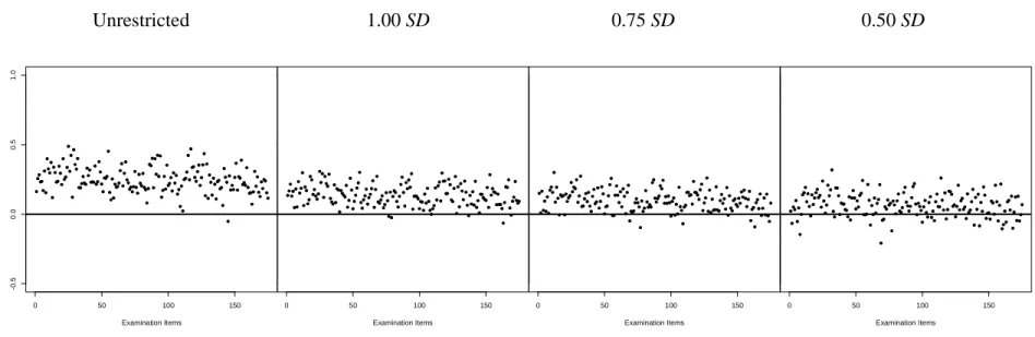
Figure 4.1 - Plots of unrestricted and restricted item discrimination values based on scores within 1.00 SD, 0.75 SD, and 0.50 SD of CX1 for Examination 1...65
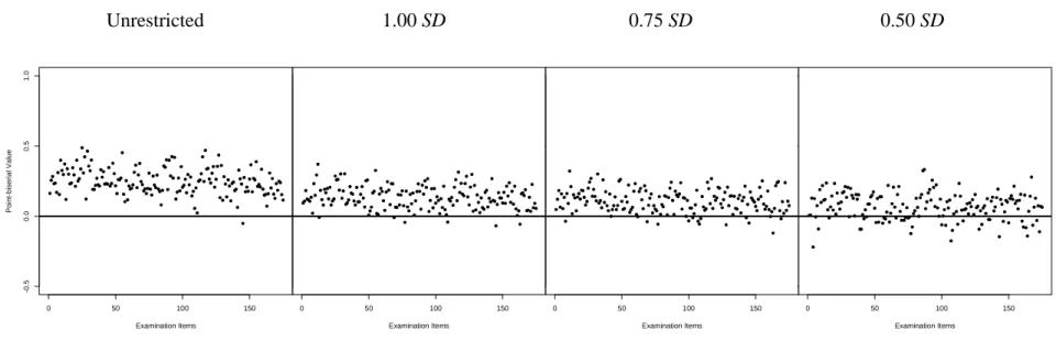
Figure 4.2 - Plots of unrestricted and restricted item discrimination values based on scores within 1.00 SD, 0.75 SD, and 0.50 SD of CX2 for Examination 1...66
Figure 4.3 - Plots of unrestricted and restricted item discrimination values based on scores within 1.00 SD, 0.75 SD, and 0.50 SD of CX3 for Examination 1...67
Figure 4.4 - Plots of unrestricted and restricted item discrimination values based on scores within 1.00 SD, 0.75 SD, and 0.50 SD of CX4 for Examination 1...68
Figure 4.5 - Plots of unrestricted and restricted item discrimination values based on scores within 1.00 SD, 0.75 SD, and 0.50 SD of CX5 for Examination 1...69
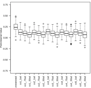
Figure 4.6 - Boxplot highlighting distribution of item discrimination values under each condition for Examination 1...70
Figure 4.7 - Plots of unrestricted and restricted item discrimination values based on scores within 1.00 SD, 0.75 SD, and 0.50 SD of CX1 for Examination 2...79
Figure 4.8 - Plots of unrestricted and restricted item discrimination values based on scores within 1.00 SD, 0.75 SD, and 0.50 SD of CX2 for Examination 2...80
Figure 4.9 - Plots of unrestricted and restricted item discrimination values based on scores within 1.00 SD, 0.75 SD, and 0.50 SD of CX3 for Examination 2...81
Figure 4.10 - Plots of unrestricted and restricted item discrimination values based on scores within 1.00 SD, 0.75 SD, and 0.50 SD of CX4 for Examination 2...82
Figure 4.12 - Boxplot highlighting distribution of item discrimination values under
each condition for Examination 2...84 Figure 4.13 - Plots of unrestricted and restricted item discrimination values based on
scores within 1.00 SD, 0.75 SD, and 0.50 SD of CX1 for Examination 3...91 Figure 4.14 - Plots of unrestricted and restricted item discrimination values based on
scores within 1.00 SD, 0.75 SD, and 0.50 SD of CX2 for Examination 3...92 Figure 4.15 - Plots of unrestricted and restricted item discrimination values based on
scores within 1.00 SD, 0.75 SD, and 0.50 SD of CX3 for Examination 3...93 Figure 4.16 - Plots of unrestricted and restricted item discrimination values based on
scores within 1.00 SD, 0.75 SD, and 0.50 SD of CX4 for Examination 3...94 Figure 4.17 - Plots of unrestricted and restricted item discrimination values based on
scores within 1.00 SD, 0.75 SD, and 0.50 SD of CX5 for Examination 3...95 Figure 4.18 - Boxplot highlighting distribution of item discrimination values under
each condition for Examination 3...96 Figure 5.1 - Pie charts representing breakdown of Form B test variant items for each
examination...129 Figure 5.2 - Pass/fail consistency tables for Examination 1
and associated test variants...131 Figure 5.3 - Pass/fail consistency tables for Examination 2
and associated test variants...132 Figure 5.4 - Pass/fail consistency tables for Examination 3
CHAPTER 1 INTRODUCTION
Examinations, and the roles they play in a variety of fields, have been the source of much debate in recent years. In the educational setting, for example, legislation like the 2001 No Child Left Behind Act (NCLB, 2002) shifted significant attention to student performance on mandatory end-of-grade examinations. The results of these examinations, depending on location, are often taken into consideration when important school-related decisions such as student retention and educator evaluation and compensation are made. In some areas, the results can even affect school and school district operating budgets.
Education is not the only field, however, in which the results of examinations can be significant and consequential. Government agencies and other professional organizations frequently require applicants for credentials to pass license- or certification-granting examinations. Lawyers, physicians, electricians, and barbers are all examples of
professionals who are required to receive government-issued licenses before being authorized to practice in their respective fields. Likewise, non-governmental entities often use
examinations as part of the process to certify persons to perform tasks or operations that require specific skill sets. An information technology company, for instance, may require technicians to pass an examination before authorizing them to work on certain software programs. Tests that are used to grant certifications or award professional recognitions are frequently referred to as credentialing examinations.
requirements are consistent among relevant parties. Adhering to these standards may also provide legal defensibility for the developers and administrators of these examinations.
The process by which credentialing examinations are developed is similar to that which is used for other types of tests. According to Downing (2006), the typical test development process is comprised of 12 steps. These steps are included in Table 1.1. The process begins with gaining an understanding of the purpose of the examination, the desired inferences to be made by test scores, as well as the general format to be used. Additional steps include defining the content to be used, creating test specifications, developing
examination items, designing and assembling the test, and test production. Following these procedures, items are frequently field-tested, scored, and analyzed to judge the
appropriateness of their inclusion in final versions of examinations. If applicable, a standard setting process may be used to recommend a minimum passing score for the test. This is followed by the development of a test reporting protocol, the establishment of an
Table 1.1
Test Development Process
Step Examples of development tasks and concerns
1. Overall plan Guidance for test development activities Confirm desired test interpretations Test format
2. Content definition Sampling plan
Content-related validity evidence 3. Test specifications Content domain sampling
Desired item characteristics 4. Item development Item writer training
Item review, editing 5. Test design and assembly Design/create test forms
Develop pretesting considerations 6. Test production Publishing/printing activities
Security/quality control 7. Test administration Standardization issues
Proctoring, security, timing issues 8. Scoring test responses Quality control
Item analysis 9. Passing scores Standard setting
Comparability of standards 10. Reporting test results Accuracy, quality control
Misuse/retake issues 11. Item banking Security issues
Usefulness, flexibility
12. Test technical report Documentation of validity evidence Recommendations
The development process for credentialing examinations can be affected by the unique characteristics these tests frequently exhibit. Unlike large-scale standardized tests used in education, credentialing examinations are often developed and administered for organizations representing occupations or fields with relatively few potential members. As such, the resources these groups are able to devote to test development and administration may be relatively limited. Although not wholly unique to credentialing examinations, examinees seeking a license or certification must also typically reach a predetermined minimum score, or cut score, in order to pass the examination and, therefore, be eligible to receive the desired credential. Tests with cut scores are also sometimes referred to as competency or mastery examinations because obtaining a score at or higher than the cut score infers examinee mastery or competency over a specified set of content standards. These attributes make credentialing examinations different than many standardized tests used in education, such as those used to measure the aptitude of prospective first-year college students. Such examinations are administered to thousands of examinees each year, creating large sets of data by which the development process is significantly aided.
The focus of this study is on one step in the process used to develop credentialing examinations. This step, frequently referred to as item analysis, is used to assess the degree to which field-tested items are suitable for inclusion in final versions of examinations. Item analysis, which Crocker and Algina (2008) defined as “the computation and examination of any statistical property of examinees’ responses to an individual test item” is included in Step 6 of Downing’s (2006) development process (p. 311). The statistical properties most
item discrimination, which measures the degree to which an item differentiates between examinees who possess more of some characteristic intended to be measured by a test (e.g., subject area mastery) and those who possess less of the characteristic. This differentiation is typically operationalized as the difference between those examinees who perform relatively well on an examination and those who perform relatively poorly.
The procedures used to calculate item discrimination values for credentialing examinations with relatively small samples of field-test data are the focus of this study. A number of statistics are currently used to gauge item discrimination. A common
Research Questions
The following research questions are addressed in this study:
1. What are the effects on item discrimination values when the values are calculated using restricted samples of examinee test scores within varying ability ranges around real or anticipated cut scores?
2. What are the effects of calculating item discrimination values based on varying ranges of examinees around cut scores on item selection, examination reliability, and classification decision consistency?
Need for the Study
The current study represents a unique contribution to the field of test development for credentialing examinations. Current procedures used to calculate item discrimination values, although appropriate and effective for many types of tests, may not be ideal for competency examinations. In addition, the study’s emphasis on tests with small samples of examinees represents the realistic—and under-studied—conditions of many testing programs,
particularly those used by credential-granting organizations. Using small sample sizes also necessitates the use of classical test theory procedures, which, despite the emergence of more sophisticated measurement models, remain popular among developers of credentialing examinations. Some of the important potential benefits of this study are described in the following paragraphs.
First, although a variety of procedures may be used to calculate item discrimination values, a common characteristic of these procedures is that they each use the entire
values. In this manner, they treat scores of examinees at both the extreme upper and lower ends of a distribution of test scores as they do scores from examinees near the examination cut score. The focus of competency examinations, however, is on candidates near the cut score. By limiting the basis for calculating discrimination values to scores of examinees near the actual or estimated cut score, greater emphasis may be applied to items that discriminate more effectively amongst examinees with ability levels closest to those for which the test was designed to distinguish.
If the sample of examinees on which discrimination values are calculated is restricted, the restriction is likely to affect the selection of items for competency examinations. It is expected that discrimination indices based on criterion groups having a narrower range of ability or performance would produce uniformly attenuated discrimination indices. However, if discrimination values based on responses within a restricted sample of examinees are significantly different than those calculated using all examinees, the items selected for an examination will be dependent on the method employed. In other words, restricting the range of test scores used to calculate discrimination values permits items that discriminate among examinees with ability levels closest to those the cut score
operationalizes to be selected over those that discriminate in other areas within the range of test scores.
Second, an important aspect of this research is that it was conducted within the context of competency examinations with relatively small numbers of examinees. Limiting the research to small-sample examinations is of particular benefit to developers of tests used to credential individuals. Unlike many large-scale educational achievement examinations for which item analysis may rely on large numbers of student responses and test scores,
credentialing tests, due to their very nature, are often limited to smaller pools of examinees. Much of the research related to item analysis has focused on tests with large numbers of examinees. Fewer, however, have examined these issues as they specifically relate to examinations with smaller samples of available test scores. Focusing the study in this manner represents a significant contribution to small-sample examination development.
CHAPTER 2 LITERATURE REVIEW
The subjects addressed in this study draw upon relevant literature from three major areas of research: (a) analyses regarding item discrimination and its role in the test
development process, (b) studies pertaining to the development of mastery or competency examinations used to credential individuals, and (c) research related to test development when relatively small samples of examinee scores are available. Significant research from each of these three areas is described in the sections that follow.
Item Discrimination and the Test Development Process
Assessing the degree to which items discriminate between examinees who possess more of some knowledge, skill, or ability and those who exhibit less is an important element in the process by which items are selected for inclusion in all types of examinations. This process, commonly referred to as item analysis, is used to compute the statistical properties of examinee responses to individual test items (Crocker & Algina, 2008). The goal of item analysis is to ensure that items selected for examinations yield levels of reliability and
Many item discrimination methods have been developed to assess the relationship between examinee responses to individual test items and test performance. Although the approaches used to calculate discrimination values according to these indices vary, they share a common purpose: to identify test items to which high-scoring examinees have a high probability of responding correctly, and to which low-scoring examinees have a low probability of responding correctly. A description of commonly used item discrimination indices is included in the sections that follow.
The index of discrimination, commonly referred to as the D-index, was one of the earliest methods developed to calculate item discrimination (Crocker & Algina, 2008). D is calculated by dividing examinees into upper- and lower-scoring groups of equal size. The criterion used to identify an examinee as belonging to either group is his or her observed test score. The proportion of examinees responding correctly to a particular item in the lower-scoring group (plower) is subtracted from the proportion of examinees responding correctly in the upper-scoring group (pupper):
D = pupper - plower (2.1)
D-values also represent the difference in average item score between the high- and low-scoring groups (Ebel, 1967).
Although D-values are mathematically simple to compute, a number of drawbacks have limited their widespread use. With no known sampling distribution, it is not possible to test for statistical significance between D-values or to identify whether a particular D-value is significantly greater than zero (Crocker & Algina, 2008). In addition, the index of
discrimination can only be used for items that are scored dichotomously. The selection of the upper- and lower-scoring groups can also significantly impact the calculated values, which may be particularly problematic for examinations with a restricted range of scores or where only small numbers of candidates are available.
When item analysis is conducted, D-values may be used to help determine the appropriateness of including individual items in the final version of an examination. Ebel (1965) developed a guideline for interpreting D-values:
1. If D is .40 or greater, the item is performing satisfactorily and no revision is required. 2. If D is between .30 and .39, little or no revision is required.
3. If D is between .20 and .29, the item needs revision. 4. If D is .19 or lower, the item should not be used.
being considered for inclusion in an examination, as, among other reasons, a low D-value may simply indicate that the item contains problematic wording.
Several studies have examined the use of variations to the index of discrimination. A classic study by Kelley (1939), for example, explored varying the size of the groups upon which D-values are calculated. Instead of using all test scores to establish upper- and lower-scoring groups, Kelley found that utilizing the upper and lower 27% of test scores produced more sensitive and stable results. Beuchert and Mendoza (1979), however, found that when sample sizes were large enough, using the upper and lower 30% or 50% of test scores produced nearly identical results to those produced by the 27% recommended by Kelley. Although Kelley, as well as Beuchert and Mendoza, addressed issues related to the current study, neither focused the calculation of item discrimination values on contiguous groups of varying sizes around examination cut scores. In addition, the researchers emphasized using groups at the extreme ends of test score distributions, a position at odds with the research presented here.
In another important study, Brennan (1972) suggested that using groups of equal size was not necessary when calculating D. Creating groups of equal size, as was done in the research described previously, was a result, according to Brennan, of “the preoccupation of test theory with the normal distribution” (p. 291). Actual score distributions for most examinations, however, are not normal. Brennan called for the creation of a new index, referred to as B, to measure item discrimination. The index is represented by the following formula:
(2.2) B=U
where U represents the number of examinees in the upper-scoring group responding correctly;
L represents the number of examinees in the lower-scoring group responding correctly; and
n1 and n2 represent the total number of examinees in the upper- and lower-scoring groups, respectively.
According to Brennan, B allows for an estimate of discrimination that does not require using groups of equal size. An important aspect of B, particularly as it relates to this research, is that it also allows evaluators to select the point along the distribution of test scores that most appropriately divides the upper and lower scoring groups:
Furthermore, regardless of the shape of the distribution of test scores, it seems reasonable to allow the test evaluator the freedom to choose the cut-off points between the upper and lower groups. Only he can determine the cut-off points that yield meaningful and interpretable upper and lower groups based upon his
consideration of the test content, student population, and overall expectations for student performance on the test. When the test constructor is free to choose the cut-off points, there is, clearly, no reason to expect that the resulting groups will be of equal size. (p. 292)
Although the calculation of discrimination values used in this research does not utilize any adaptation of D or B, Brennan’s claim that the most appropriate method used to calculate item discrimination values may be examination-dependent is relevant. A major consideration in this study is that the focus of mastery examinations is the test cut score. It appears reasonable, therefore, to use the cut score as the central point in the distribution of test scores upon which discrimination values are estimated.
discrimination. These methods are used to calculate the degree to which item performance and overall test performance are correlated. Two of the more commonly used correlational indices are the point-biserial correlation and the biserial correlation. Although both of these indices utilize correlation statistics to describe discriminating power, the results they produce are different. A brief description of each index is included in the paragraphs that follow.
The point-biserial correlation is the observed correlation between examinee
performance on a dichotomously scored item and overall test score (Livingston, 2006). For dichotomously scored items, correct responses are scored 1 and incorrect responses are scored 0. The observed correlation between item response and test performance forms the basis for the biserial correlation. Like all correlation coefficient values, the point-biserial values range between -1.00 and 1.00. Negative values represent items that
discriminate negatively, while positive values represent those that discriminate positively. Larger values represent items with greater levels of discriminating power.
The point-biserial statistic, rpbis, may be calculated using the following formula:
rpbis=(µ
+−µx)
σx
p / q (2.3)
where µ+ is the mean total score for those who respond to the item correctly; µx is the mean total score for the entire group of examinees;
σx is the standard deviation for the entire group of examinees; p is item difficulty; and
A common criticism of the point-biserial statistic is that it may sometimes be spurious because the item score contributes to the total score for each examinee. This can result in inflated discrimination values. The effect is greatest for examinations with relatively few items, resulting in a curious situation in which shorter examinations, which typically produce lower levels of reliability, exhibit higher item discrimination values (Burton, 2001). For examinations with more than 25 items, such as those used in this study, however, the effect is rarely problematic and does not significantly affect discrimination values (Crocker & Algina, 2008).
The biserial correlation index produces results similar to the point-biserial index, but is calculated in a slightly different manner. The biserial, which was first derived by Pearson (1909), treats scores on dichotomously scored items as indicators of an unobservable
underlying proficiency. The biserial estimates the correlation between this latent underlying proficiency and total test score.
The biserial statistic, rbis, may be calculated using the following formula:
rbis=(µ
+−µx)
σx
( p / Y ) (2.4)
where µ+ is the mean total score for those who respond to the item correctly; µx is the mean total score for the entire group of examinees;
σx is the standard deviation for the entire group of examinees; p is item difficulty; and
In general, the biserial statistic produces larger discrimination values than those produced by the point-biserial. This is due to the fact that the Y ordinate on the normal curve, which is used to calculate the biserial, will always be larger than pq, which is used to calculate the point biserial (Lord & Novick, 1968). The differences are more profound when item difficulty values are less than 0.25 or greater than 0.75. Differences in item
discrimination values, therefore, may be attributed not only to qualitative differences among examination items, but also to the statistic used to estimate the level of discrimination.
Item response theory, a general statistical theory that relates performance on test items to the abilities the test is intended to measure, may also be used to calculate item discrimination values (Hambleton & Jones, 1993). At its core, item response theory
estimates the probability that particular examinees will respond in certain ways to items with certain characteristics (Yen & Fitzpatrick, 2006). Although the Rasch, or one-parameter logistic model, provides estimates for item location (i.e., item difficulty) only, the two- (and greater) parameter logistic models estimate difficulty and item discrimination. The
discrimination estimate produced by item response theory models is analogous to the item-total correlation statistics (i.e., the biserial and point-biserial) used in classical test theory.
Item response theory is also computationally more complex than the classical test theory discrimination indices mentioned earlier. The two-parameter logistic model uses two parameters to describe each item. These parameters include item difficulty, bi, and item discrimination, ai. The estimates may be calculated using the following equation:
(2.5)
Pi(Xi=1θ)= 1
where Pi represents the probability of a correct response ( ability level (θ); and
D represents a multiplicative constant, typically set at either 1.7 or 1.702 (Yen & Fitzpatrick, 2006).
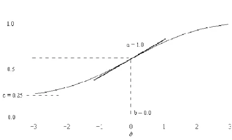
When the parameters are plotted, they create what are commonly referred to as item characteristic curves (ICCs). The
ICC, with steeper slopes indicating greater levels of item discriminati example of an ICC produced using a three
representing examinee noise or guessing, is shown in Figure 2.1. In the figure, the slope, labeled a, represents item discrimination.
Figure 2.1. Example of item characteristic curve (ICC)
represents the probability of a correct response (Xi = 1) given a particular
represents a multiplicative constant, typically set at either 1.7 or 1.702 (Yen &
When the parameters are plotted, they create what are commonly referred to as item characteristic curves (ICCs). The ai, or discriminating parameter, specifies the slope of the ICC, with steeper slopes indicating greater levels of item discrimination (Luecht, 2006). An example of an ICC produced using a three-parameter logistic model, with the third parameter representing examinee noise or guessing, is shown in Figure 2.1. In the figure, the slope,
, represents item discrimination.
. Example of item characteristic curve (ICC)
= 1) given a particular
represents a multiplicative constant, typically set at either 1.7 or 1.702 (Yen &
When the parameters are plotted, they create what are commonly referred to as item , or discriminating parameter, specifies the slope of the
Estimates produced using item response theory require larger sample sizes than those produced using classical test theory. Reise and Yu (1990), for example, found that at least 500 cases were needed to produce dependable item parameter estimates, including item discrimination, when using item response theory, with 1,000 to 2,000 cases required for more accurate estimates. Hambleton and Jones (1993) found that the number of cases required to effectively utilize item response theory depended on the particular model being used; however, in general, they recommended no less than 500 cases be used. Despite its advantages, therefore, when calculating discrimination values, developers of examinations for which relatively small samples of examinee responses are available must typically rely on classical test theory procedures, such as the biserial or point-biserial item-total correlation statistics.
Much of the research associated with item discrimination and its role in the test development process has focused on comparisons between the various indices. Beuchert and Mendoza (1979), for example, analyzed the results of eight studies that compared
discrimination values produced by a number of indices. Four of the studies found the values to be virtually indistinguishable. The others found minor, but sufficiently significant,
nonexistent in situations intended to accentuate those differences” (p. 116). Based on these results, Beuchert and Mendoza recommended using the most computationally simple index.
In a related study, Oosterhof (1976) compared discrimination values produced by 19 different indices using exploratory factor analysis. His research found the loadings
representing each of the discrimination indices to be “impressively high,” with six indices exhibiting loadings greater than 0.98 and all but one with loadings greater than 0.85 when loaded against a single common factor (p. 149). Oosterhof summarized his findings in the following manner:
When any of the selected indices are used to evaluate the relative performance of an item, the preference of one index over another minimally affects the resulting analysis. Preference towards a particular index would more appropriately be based on convenience of calculation or intuitive preference. It is inappropriate to suggest that using any of the common indices included in the present study has an appreciable effect on the eventual outcome of an analysis. (p. 149)
A more recent study by Fan (1998) compared the results of item analysis using both item response theory and classical test theory for a 108-item examination given to over 190,000 high school students in Texas. Fan estimated item discrimination values for each item using a two- and three-parameter logistic item response theory model and the point-biserial statistic. The majority of correlation coefficients for the discrimination values ranged between 0.60 and 0.90. Although this relationship was somewhat weaker than that found for differences in item difficulty values, which was also assessed in the study, Fan indicated that the overall relationship between discrimination values calculated using item response theory and classical test theory to be “moderately high to high” (p. 378). According to Fan,
Fan’s findings are similar to conclusions reached by Thorndike (1982), who, in discussing the then relatively new use of item response theory in test development procedures, wrote:
For the large bulk of testing, both with locally developed and with standardized tests, I doubt there will be a great deal of change. The items that we will select for a test will not be much different from those we would have selected with earlier procedures, and the resulting tests will continue to have much the same properties. (p. 12)
Additional research associated with item discrimination has introduced new or modified versions of previously established indices. Harris and Subkoviak (1986), for example, developed a new index of discrimination, referred to simply as the agreement index. In developing the index, the authors hoped to create a procedure that incorporated certain aspects of item response theory, but which was computationally less complex. Designated P(Xc), the agreement may be calculated using the following formula:
P(Xc)=a
11−a22
N (2.6)
where a11 represents the number of examinees responding to an item correctly; a22 represents the number of examinees responding incorrectly; and
N represents the total number of examinees.
P(Xc) can be interpreted as the probability of agreement between performance on a single item and performance on the overall examination, with ideal items having values equal to 1.00.
of 30, 50, and 100 items, and numbers of examinees, ranging between 30, 60 and 120. The results indicated that the average correlation between items selected using these two methods was 0.91. According to the authors, the correlation was sufficiently strong as to recommend the use of the agreement index, as estimates are much easier to compute than when using the two-parameter logistic model.
Credentialing Examinations
In many instances, examinations are developed for the purpose of classifying examinees into two or more groups. These types of tests, also frequently referred to as mastery or competency examinations, are used in a variety of fields. Competency
examinations are used in education, for example, to identify students who may need remedial instruction, or to determine fitness for graduation. As such, they are not norm-referenced, as many achievement examinations used in education are, but rather are criterion-referenced; that is, examinees must meet specified standards, as operationalized by a pre-determined score, in order to pass. Government agencies and other professional organizations use mastery examinations to credential individuals in a variety of fields and occupations. Doctors, lawyers, and teachers, for example, must pass competency examinations before receiving the credentials they need to practice in their respective fields.
these programs require the candidates to pass a competency examination. In contrast to licensure programs, certification programs are not government-regulated, but rather are typically managed within an occupational field and are usually voluntary. A certification attests to the fact that the individual has met a credentialing organization’s standards and is entitled to make the public aware of his or her professional competence.
A primary purpose behind using competency examinations as a requirement for granting credentials, both government-regulated licenses and certifications, is ensuring that individuals are properly qualified to practice in their respective fields. The requirement made by many states for certain occupations to obtain licensure is also driven by the desire to promote public safety. According to the Standards (AERA et al., 1999):
Tests used in credentialing are intended to provide the public, including employers and government agencies, with a dependable mechanism for identifying practitioners who have met particular standards. Credentialing also serves to protect the profession by excluding persons who are deemed to be not qualified to do the work of the
occupation. Tests used in credentialing are designed to determine whether the essential knowledge and skills of a specified domain have been mastered by the candidate. (p. 156)
Government and professional organizations have used examinations to regulate a variety of occupations for hundreds of years. Chinese civil servants, for example, have been required to pass written examinations for nearly three millennia, with similar requirements for the medical and legal fields in place sometime before 500 B.C.E. (DuBois, 1970). Modern use of credentialing examinations originated, to a large degree, in the medical field. Garcia-Ballester, McVaugh, and Rubio-Vela (1989) listed several factors behind the rise of government-regulated standards in the medical field. Among these included: a concern for quality healthcare; a desire to restrict access to the field to those already practicing, in essence creating a monopoly for current practitioners; and political confrontations over the power to regulate certain occupations.
Today, government agencies continue to regulate an ever-growing number of fields. Atkinson (2012) listed the occupations in each state that required licensure as of 2010. California, at the top of the list, licensed 177 professions. Nine additional states licensed over 100 occupations each. Missouri, the state with the fewest number of licensed
Table 2.1
States with Most and Fewest Licensed Occupations
Rank State Licensed Rank State Licensed Occupations Occupations
1 California 177 41 Colorado 69 2 Connecticut 155 42 North Dakota 69 3 Maine 134 43 Mississippi 68 4 New Hampshire 130 44 Hawaii 64 5 Arkansas 128 45 Pennsylvania 62 6 Michigan 116 46 Idaho 61 7 Rhode Island 116 47 South Carolina 60 8 New Jersey 114 48 Kansas 56 9 Wisconsin 111 49 Washington 53 10 Tennessee 110 50 Missouri 41 Note. Information derived from Atkinson (2012).
as possible” (p. 6). Appropriately, therefore, the Standards (AERA et al., 1999) recommend that those responsible for setting standards be “concerned that the process by which cut scores are determined be clearly documented and defensible” (p. 54).
The process used to develop cut scores is referred to as standard setting. Although a thorough review of the many standard-setting methodologies currently in use is beyond the scope of this study, a brief and general description of typical standard setting procedures is warranted. During standard setting conferences, subject matter experts, who are also frequently referred to as judges or participants, review definitions of the knowledge, skills, and attributes examinees must possess to be deemed minimally qualified for inclusion in a particular proficiency category. For many examinations, these categories may simply represent those who pass the test, and those who do not. Depending on the standard setting method used, the participants then make judgments about either individual examinees or individual test items. Through a variety of method-dependent procedures, the participants’ judgments are translated into a recommended cut score. Once approved by the examination’s governing body, candidates must score at or above the cut score in order to pass the test.
The accuracy of classifications made when utilizing credentialing examinations with cut scores is, of course, critically important. Because of this, more focus is given to ensuring precision around the cut score. According to the Standards (AERA et al., 1999):
Tests for credentialing need to be precise in the vicinity of the passing, or cut, score. They may not need to be precise for those who clearly pass or clearly fail. Sometimes a test used in credentialing is designed to be precise only in the vicinity of the cut score. (p. 157).
The above quote is of particular relevance to the current study. As discussed
the scores upon which discrimination values are calculated to those near the cut score, more precision is applied to those for whom the accuracy of the cut score is most relevant and consequential.
The knowledge and skills needed to practice in licensed fields changes periodically. In many instances advances in technology or methods of practice drive these changes. As such, the examinations used to credential individuals in these fields must also be altered to reflect the changes. When such changes occur, the examination cut score must also be reevaluated. Again, the Standards (AERA et al., 1999) describe the importance of this process:
Practice in professions and occupations often change over time. When change is substantial, it becomes necessary to revise the definition of the job, and the test content, to reflect changing circumstances. When major revisions are made in the test, the cut score that identifies required test performance is also reestablished. (p. 157)
In addition to research associated with the establishment and use of cut scores, the literature related to credentialing examinations has also emphasized issues related to examination validity and reliability. Researchers have focused on how these principles, critical to the development of any test, specifically relate to credentialing examinations.
According to the Standards (AERA et al., 1999), test validity is “the degree to which evidence and theory support the interpretation of test scores entailed by proposed uses” (p. 9). The interpretation of test scores produced by credentialing examinations is that
examinees who pass the test are qualified to receive the associated credential and, therefore, are qualified to practice in their respective fields. According to Clauser et al. (2006):
Obtaining the evidence necessary to support claims of examination validity is referred to as test validation. Cizek (2012b) summarized this process:
Validation is the ongoing process of gathering, summarizing, and evaluating relevant evidence concerning the degree to which that evidence supports the intended meaning of scores yielded by an instrument and inferences about standing on the characteristic it was designed to measure. (pp. 35-36)
As it specifically relates to credentialing examinations, gathering validity evidence can, at times, be somewhat challenging. Whereas the degree to which credentialing tests accurately classify examinees is the critical validity concern, it follows that a thoughtful analysis of this question might compare the performance of examinees who pass the
examination with those who fail. Examinees who fail, however, are typically not allowed to practice in the field, and, therefore, such comparisons are normally not possible (Clauser, Margolis, & Case, 2006).
A more realistic approach to gathering validity evidence for credentialing examinations may be one in which evidence supporting the appropriateness of the examination’s interpretive argument is identified. According to Kane (1992):
A test-score interpretation always involves an interpretive argument, with the test score as a premise and the statements and decisions involved in the interpretation as conclusions. The inferences in the interpretive argument depend on various
examination content realistically reflects the knowledge and skills needed by those seeking licensure or certification.
Raymond and Neustel (2006) underscored the importance of ensuring that the content associated with credentialing examinations reflected requirements for safe and effective practice in the fields for which credentials are awarded. According to the authors, this can be accomplished through the use of practice analyses, which “identify the job responsibilities of those employed in the profession” (p. 181). After conducting these analyses, the knowledge, skills, and attributes of the associated responsibilities may be obtained. These, in turn, aid developers in establishing a test blueprint, or specification. Raymond and Neustel listed several useful tools to aid in the conduct of practice analyses, including task inventory questionnaires, task statements, and job responsibilities scales.
Although the majority of their study evaluated various methodologies used to ensure appropriate content, Raymond and Neustel (2006) also highlighted the importance of using empirical data, such as computed “statistical indices of item-domain congruence…” to inform the item selection process (p. 206). This process, inevitably, includes an analysis of the discriminating power of potential examination items.
Clauser et al. (2006) also examined methods used to identify appropriate content for credentialing examinations. Like Raymond and Neustel (2006), the authors emphasized the importance of generating job responsibility inventories. In order to limit the size and scope of the examination, however, Clauser et al. suggested restricting task inventories to those activities that ensured public safety:
Reliability is also the focus of considerable research related to credentialing examinations. Put simply, examination reliability is the “desired consistency (or reproducibility) of test scores” (Crocker & Algina, 2008, p. 105). Over time, several methods have been developed to measure reliability. Early procedures relied on
administering the same examination multiple times. Utilizing the test-retest method, for example, the developer administers an examination to a group of examinees, waits a predetermined amount of time, and then re-administers the examination. The correlation between examinee test scores, referred to in this context as the coefficient of stability, is then calculated (Crocker & Algina, 2008). Similar methods require administering alternate test forms to examinees and calculating the correlation between scores on the forms.
Other approaches used to estimate reliability rely on single administrations of examinations. One such procedure is the split-half method, in which a single examination form is administered to a group of examinees. Before the test is scored, however, the examination is divided into two equivalent halves. The halves are scored as if they were separate examinations, and the correlation between test scores is calculated for each
examinee. The method assumes that the halves are strictly parallel. In addition, because the split-half tests contain fewer items than the whole examination, the coefficient
underestimates the reliability of the full-length test. The Spearman Brown correction was designed to overcome this problem (Crocker & Algina, 2008).
commonly referred to as Cronbach’s alpha, or coefficient alpha, can be calculated using the following formula:
(2.7)
where k is the number of items on the examination; is the variance of item i; and
is the total test variance (Crocker & Algina, 2008).
Using coefficient alpha, it is possible to treat each test item as a subtest and, therefore, to estimate the degree of reliability between the subtests.
Although coefficient alpha is commonly used as an estimate of reliability for all types examinations, including those used to credential individuals, the literature suggests that other forms of reliability estimates may also be appropriate when an examination is used to make classification decisions. According to Haertel (2006):
When continuous scores are interpreted with respect to one or more cut scores, conventional indices of reliability may not be appropriate, and the standard error of measurement may not be directly informative concerning classification accuracy. Such cases arise when examinees above a cut score are classified as passing or proficient, for example. Instead of standard errors, users may be concerned with questions such as the following: What is the probability that an examinee with a true score above the cut score will have an observed score below the cut score, or
conversely? What is the expected proportion of examinees who would be differently classified upon retesting? (p. 99)
Classification decision consistency indices have been developed to measure the degree to which the same decisions are made from two different sets of measurements. One of the earliest indices, referred to simply as , can be explained using a two-by-two table,
ˆ
α= k
k -1
1-∑σˆi2
ˆ
σx2
ˆ
σ
i2ˆ
σ
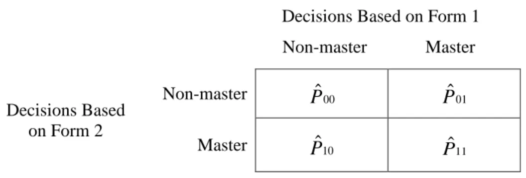
x2similar to that shown in Figure 2.2. The cells in the table represent the proportions of
examinees who are classified as either masters or non-masters after taking different forms of the same examination. The cell labeled , for example, represents the proportion of examinees classified as masters by both forms. The cell labeled represents the
proportion of examinees classified as masters using the first form, but as non-masters using the second form.
Decisions Based on Form 1 Non-master Master
Decisions Based on Form 2
Non-master Master
Figure 2.2. Probabilities of consistent classifications using two forms (Crocker & Algina, 2008)
The estimated probability of a consistent decision, therefore, can be calculated using the following formula:
ˆ
P
=
P
ˆ
11+P
ˆ
00 (2.8)Values for can range between 0.00 and 1.00, with 0.00 representing complete inconsistency and 1.00 representing total consistency.
ˆ P11
ˆ
P
10ˆ
P
00P
ˆ
01ˆ
P
10 Pˆ11Although was recommended as a measure of classification decision consistency (Hambleton & Novick, 1973), the index is not without flaw. For example, a value greater than 0.00 would be expected by chance, even if the measurements used were uncorrelated. In an effort to overcome this situation, Swaminathan, Hambleton, and Algina (1974) recommended using Cohen’s (1960) κ as a measure of classification decision consistency. The coefficient can be calculated using the following formula:
(2.9)
where Pc, also referred to as the chance consistency, is the probability of a consistent decision, and may be calculated using the following formula:
(2.10)
The four elements used to calculate Pc represent the margin sums in the hypothetical table displayed in Figure 2.2. That is, P1. represents the probability of a mastery classification on one form and P.1 represents a similar probability on the other form. The same holds true for P0. and P.0, which represent misclassifications on the forms. The interpretation of
κ
is somewhat different than that of , as it represents the increase in decision consistency over that expected by chance. The coefficient is 0.00 when there is no increase, and 1.00 when there is maximum increase (Crocker and Algina, 2008).A limitation of the classification decision consistency indices discussed thus far is
ˆ P
κ=P−Pc
1−Pc
Pc=P1.P.1+P0.P.0
developed procedures by which P and could be estimated from a single administration. The approaches produce estimates using a hypothetical form that is exchangeable with the examination from which data is gathered (Crocker & Algina, 2008). Huynh’s method has been shown to produce fairly accurate estimate of P and for parallel tests with as few as 10 items (Subkoviak, 1978).
Issues related to the validity and reliability of credentialing examinations are also significant when the legal defensibility of such tests are considered. According to Atkinson (2012), “as the number of regulated professions which use an examination as one criterion of eligibility increases so will the likelihood of a legal challenge” (p. 506). Although much of the attention competency examinations receive is on the score that defines passing and
failing, Atkinson found that legal challenges rarely contest the cut scores themselves. Rather, legal challenges are focused on the entire test development process. According to Atkinson: “The basis for legally substantiating an examination program and its Pass/Fail determination discriminating between those recognized as establishing competence and those who have not, will necessitate an analysis of the entire examination development…” (p. 511).
Legal defensibility is an important consideration within the context of the current study because item analysis, including the calculation and evaluation of item discrimination values, is a critical step in the test development process. If calculating discrimination values using only restricted samples of examinee responses is more appropriate for credentialing examinations, the issue becomes relevant to the test’s defensibility.
Very few studies have assessed the role item discrimination plays in the development of credentialing examinations. Although not specific to credentialing tests, Harris and Subkoviak (1986) discussed the importance of item discrimination in the development of
κ
mastery examinations in general. They advocated developing tests that maximize score differences between groups who pass and fail, while simultaneously minimizing score differences within these groups:
For a mastery test, this means selecting items that discriminate between masters and non-masters, as opposed to within masters and within non-masters. The consensus appears to be that a good mastery item is one which masters answer correctly and non-masters answer incorrectly. (p. 496)
More closely related to the current study, Buckendahl and Davis-Becker (2012) conducted research regarding the establishment of passing standards for credentialing
Test Development with Small Samples of Examinee Responses
An important aspect of the current study is that is utilizes tests for which relatively small numbers of examinee responses are available for item analysis. As discussed earlier, this is a realistic condition under which many credentialing examinations are developed. Jones, Smith, and Talley (2006) characterized this situation as one in which fewer than 200 examinee responses were available for analysis “either because the testing program is new or because the target population is inherently small” (p. 487).
A primary consideration in such situations is the process by which field-test data may be gathered for further analysis. According to the Standards (AERA et al., 1999), this process should be documented and should utilize examinees drawn from the population for which the examination was constructed:
When item tryouts or field tests are conducted, the procedures used to select the sample(s) of test takers for item tryouts and the resulting characteristics of the sample(s) should be documented. When appropriate, the sample(s) should be as representative as possible of the population(s) for which the test is intended. (p.44) According to Jones et al. (2006), for examinations with relatively small numbers of possible test takers, this recommendation can be challenging because the developer must be in a position “to make sound statistical inferences while working within the constraints imposed by the testing system; namely, that there are fewer than 200 test takers available to participate in field testing – perhaps far fewer” (p. 493).
Millman and Greene (1989) suggested starting with a preliminary tryout of test items given to as few as five or six members of the target population or subject matter experts. The tryout would be followed by interviews aimed at ascertaining the examinees’ thoughts
examinees are available. They suggested recruiting a stratified sample of examinees that is distributed similarly to the projected population. Such a strategy can help ensure that the sample is diverse enough to allow for a meaningful evaluation of the items’ discriminating properties.
Once field-test data is collected, a determination regarding the appropriate
measurement model to use must be made. As discussed previously, in many cases, analysis of items may be limited to classical test theory, as other models, such as item response theory, require larger numbers of examinees. Jones et al. (2006) examined the potential use of various measurement models under three different conditions: (a) when there are no pretest data, (b) when a pretest sample up to N = 100 is available, and (c) when a pretest sample of N = 100 to 200 is available.
According to Jones et al. (2006), when no item response data is available, developers must rely on rigorous item review procedures that emphasize item appropriateness, alignment with test specifications, content domain representativeness, potential item bias, and the adequacy of instructions. The previously described recommendation by Millman and Greene (1989), that the items may be administered to a handful of subject matter experts, may also be beneficial. Thorndike (1982) suggested that item difficulty and discrimination parameters might be estimated using regression analysis. This approach requires previously used items with known item parameters as well as judges who estimate the difficulty of new items.
sample statistics when N was as small as 40. According to Jones et al., “In the end, if the item pool is small, sample sizes as low as N = 50 may provide enough information to select desirable test items for inclusion in new test forms” (p. 506). The authors also discussed the use of item response theory for samples in this range. For tests being developed on N ≤ 100 examinee responses, they found that the one-parameter logistic model could be effective in estimating item difficulty. The one-parameter model, as discussed earlier, however, holds all discrimination values as equal, and, therefore, is not appropriate for studies investigating the role of discrimination in item selection.
Finally, for sample sizes of N = 100 to 200, Jones et al. (2006) found that classical test theory and item response theory procedures produced stable item parameters, which “facilitates making reliable item selection decisions within a larger item pool” (pp. 506-507).
In addition to the research conducted by Jones et al. (2006), other studies have compared the utility of classical test theory and item response theory in dealing with small-scale examinations. Not surprisingly, for examinations with 200 or fewer examinee responses, most suggest using classical test theory. Hambleton and Jones (1993), for example, found that whereas the number of cases required to use item response theory
depended, to a certain extent, on the model being employed, at least 500 cases were desired.
Summary
The preceding sections described the relevant literature in three areas: (a) research related to item discrimination and its role in the test development process, (b) the
CHAPTER 3 METHOD
Three examinations were used to measure the effect restricting scores upon which item discrimination values were calculated to those near cut scores had on the discrimination values themselves, item selection, examination reliability, and classification decision
consistency. Detailed information regarding participants, materials used, and data analysis procedures are included in the sections that follow.
Participants
The participants in this study were examinees who took one of three tests used to credential individuals in health-related professions. As seen in Table 3.1, the number of participants varied according to examination. Utilizing examinations with various examinee population sizes allowed for a closer analysis of how the dependent variables were affected by sample size. The examinations used were also selected because the examinee population size for each is relatively small, reflecting realistic conditions under which many
credentialing examinations are developed. In each case, the examinee population size is N ≤
Table 3.1.
Summary of Examination Characteristics
Number of
Examination Type Stakes N Items Scoring Timing
Examination 1 C M 490 175 D 8 hours Examination 2 C M-H 161 200 D 4 hours Examination 3 C L 76 175 D 4 hours Note. The following legend explains the symbols used in this table:
N = sample size; Type: C = certification; Stakes: L = Low, M = Medium, H = High; N = number of examinees; Scoring: D = dichotomous; Timing: number of hours permitted.
Materials
Three examinations were used in this study. Each examination was used to credential individuals in a health-field profession. Responses to test items were used to answer the research questions. A brief description of each examination used is included in the following sections.
Examination 1
were given eight hours to complete the test. The examination is accredited by the American National Standards Institute (ANSI, 2013), which ensures it meets internationally recognized standards pertaining to certification of personnel. The examination, which is offered
internationally, is considered to have low to medium stakes, with certification influencing some employment decisions. Descriptive statistics for Examination 1 (as well as for the other examinations used in the study) are included in Table 3.2. In addition, histograms representing total score distributions for Examinations 1, 2, and 3 are included in Figures 3.1, 3.2, and 3.3, respectively.
Figure 3.1. Histogram of total scores for Examination 1. Examination 1 Total Score
F
re
q
u
e
n
c
y
0 50 100 150 200
0
2
0
4
0
6
0
8
0
1
0
0
1
2
0
1
4