Efficient Global Penetration Depth Computation for Articulated Models
Hao Tiana, Xinyu Zhanga, Changbo Wanga, Jia Panb, and Dinesh Manochac
aSchool of Software, East China Normal University, Shanghai, China. bThe University of Hongkong.
cThe University of North Carolina at Chapel Hill.
Abstract
We present an algorithm for computing the global penetration depth between an articulated model and an obstacle or between the distinctive links of an articulated model. In so doing, we use a formulation of penetration depth derived in configuration space. We first compute an approximation of the boundary of the obstacle regions using a support vector machine in a learning stage. Then, we employ a nearest neighbor search to perform a runtime query for penetration depth. The computational complexity of the runtime query depends on the number of support vectors, and its computational time varies from 0.03 to 3 milliseconds in our benchmarks. We can guarantee that the configuration realizing the penetration depth is penetration free, and the algorithm can handle general articulated models. We tested our algorithm in robot motion planning and grasping simulations using many high degree of freedom (DOF) articulated models. Our algorithm is the first to efficiently compute global penetration depth for high-DOF articulated models.
Keywords: Configuration Space, Articulated Models, Penetration Depth, Support Vector Machine
1. Introduction
Computing the magnitude of inter-penetration between two overlapping rigid/articulated objects is a fundamental problem in computational geometry. One metric that is widely used to measure the extent of inter-penetration is penetration depth (PD), which requires computing a minimum transformation (translation and rotation) to separate two overlapping object-s. The resulting transformation motion can be used to com-pute the contact force for penalty-based methods, valid poses in grasping simulations, force/torque feedback in haptic render-ing, sample generation in narrow passages for motion plannrender-ing, etc.
The exact computation for PD, particularly the so-called gen-eralized PD that involves both translation and rotation [1], can be reduced to arrangement computation in a high-dimensional configuration space that has high computational complexity. For instance, the combinatorial complexity of exact PD is as high as O(n12) [2] for two models with ntriangles in three-dimensional space. As a result, all practical algorithms tend to compute an approximate solution. A wide variety of algo-rithms have been proposed in the literature for rigid models (e.g [3, 4, 2, 5, 6, 7, 8]). For articulated models, the resulting con-figuration spaces are high-dimensional non-Euclidean spaces. For instance, the configuration space for a stationary obstacle and a six degrees of freedom (DOFs) robot arm fixed on the ground, is a six-dimensional non-Euclidean space. If we allow the arm base to move in space, its configuration space becomes nine-dimensional and non-Euclidean. As the number of joints
Email address:[email protected].(Xinyu Zhang)
increases, the complexity of a configuration space can become very high. In particular, if self-collisions between distinctive links must be considered, the complexity can increase rapidly. These self-collisions may correspond to many small and iso-lated components in the high-dimensional configuration space. Due to its high complexity, it is challenging to produce an exact representation of a space with such high dimensionality. To the best of our knowledge, only one recent study [9] has attempt-ed to compute PD between articulatattempt-ed models, but its solution yielded only locally optimal PD.
Main Result:We present an efficient algorithm to approximate the global PD in high-dimensional spaces for articulated mod-els. Built on the early framework proposed in [8, 10], we use a machine learning method to approximate the boundary of the obstacle regions in the configuration space for an articulated model and its surrounding obstacles. We generate a set of con-figuration samples to densely cover the boundary of obstacle regions. Given a query configuration for computing PD, the closest configuration can be found quickly using approximate
k-nearest-neighbor search. The magnitude of PD can be com-puted using non-Euclidean distance metrics between the query configuration and the closest configuration. Compared with ex-isting methods, our method has the following advantages:
Novelty: Our algorithm is the first global PD approach for high-DOF articulated models.
Generality: Our algorithm can handle hybrid joints and links represented using polygonal models.
plan-ning, and grasping simulation.
Efficiency: Our algorithm takes about 0.03∼3 milliseconds per runtime PD query on single core. The computational complex-ity of runtime query depends only on the number of support vectors used in learned obstacle regions.
The rest of the paper is organized as follows. In Section 2, we provide a review of the related work on PD computation. In Section 3, we introduce the notation that we use in the paper and present the algorithm for approximating obstacle regions for articulated models. In Section 4, we describe our approach to compute PD by using approximate obstacle regions and a solution for computing conservative PD. Section 5 describes the implementation details and some basic experimental results. Section 6 highlights the results on complex scenarios.
2. Related Work
There are two types of PD: translational PD and generalized PD. Translational PD corresponds to a translational motion to separate two objects, whereas generalized PD corresponds to both translational and rotational motions. Various work on PD computation has been reported in computer graphics, geomet-ric modeling, haptics, and robotics, and most of the associated algorithms address rigid models. In the following, we offer a brief overview of these algorithms.
Translational Penetration Depth: Exact translational PD can be formulated using the Minkowski sum; it is obtained by computing the closest distance from the origin to the bound-ary of the Minkowski sum [11, 12]. The worst-case complex-ities for these approaches is O(n2) for convex polytopes and
O(n6)for non-convex polytopes, wherenis the number of fea-tures in the polytopes [11]. Because of the high computational cost involved in computing exact translational PD, most prac-tical approaches compute an approximation instead. For con-vex polytopes, many methods simply compute an approximate Minkowski sum, which is then used as an approximate transla-tional PD calculation [13, 14]. Translatransla-tional PD between non-convex objects is typically computed using non-convex decomposi-tion, which is based on the fact that an exact Minkowski sum can be computed based on convex decomposition and the u-nion of all the pairwise Minkowski sums [15]. As it is expen-sive and not particularly robust to compute the union explic-itly, many approximate solutions have been proposed, includ-ing GPU-based approaches [2, 16] and methods that are based on reduced convolution and filtering [17, 18]. Other method-s avoid the expenmethod-sive Minkowmethod-ski union entirely by comput-ing only translational PD between each pair of convex com-ponents. These approaches are called local methods because the resulting PD only depends locally on the closest point on the penetrated surfaces and may not result in a globally con-sistent solution. Most local PD methods are based on local features [19, 20, 18, 21, 22], i.e., each convex piece generated by the convex decomposition is a mesh triangle. Some recent methods [7] uses iterative optimization to compute approximate translational PD.
Generalized Penetration Depth: Few algorithms can com-pute generalized PD, which considers both translation and
ro-tation. [1] estimate the upper and lower bounds for general-ized PD between two general polyhedral models by decom-posing the models into convex components. Most practical al-gorithms for generalized PD computation follow the iterative, constrained optimization framework, which generates a series of configurations on the contact space with decreasing distances to the given in-collision query. [5] generates such a series of configurations by moving a small step size from a configura-tion along the gradient direcconfigura-tion. [6] first compute an approx-imate local contact space near a configuration and then perfor-m randoperfor-m saperfor-mpling within the approxiperfor-mate contact space to find a suitable following configuration. [23] calculate a lin-earized contact space in the neighborhood of a configuration and then obtain an optimal following configuration by solving a linear complementary problem (LCP). Most of these approach-es [1, 6, 5] are slow for interactive applications and do not have the necessary guarantees for a global solution.
Penetration Depth for Articulated Models: Recently, [9] present an algorithm to approximate PD for articulated models. Their algorithm approximated a local configuration space using iterative and constrained optimization techniques and provided a locally optimal PD.
Other Penetration Depth Metrics: In addition to the relat-ed work above, there are other definitions of PD. Intersection volume and its derivative can also be used for volume-based re-pulsion [24]. Distance fields are also used for local translational PD computation [25] and can be computed in realtime using G-PUs. Point-based Minkowski sum approximation [26] can also be used to compute translational PD.
3. Configuration Space Approximation
3.1. Notation
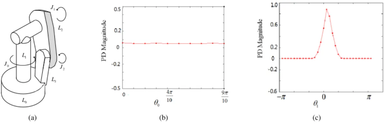
We denote an articulated model asAand an obstacle asO, as shown in Fig. 1. We assume that A has n links. The i -th link of Ais denoted as Li, and the link attached toLi is denoted asLi+1. The joint connecting two links,LiandLi+1, is denoted asJi. JointJi’s parameter is denoted asθi. We denote the configuration space composed ofAandOas Cand each configurationqinCcorresponds to the relative configuration (i.e., translation and rotation) ofAwith respect toO. Thei -th component ofqisqi=θi. Chas two regions: the obstacle region Cobs ={q:A(q)∩ O,∅} and free space Cf ree=C \ Cobs. Intuitively speaking,Cobscorresponds to configurations in whichAandOcollide, andCf reecorresponds to configurations in whichAandOdo not. If self-collisions between distinctive articulated links are considered and added to the definition of
Cobs, we can rewriteCobs={q:A(q)∩ O,∅} ∪ {q:Li(q)∩ Lj(q),∅,|i−j|>1}. Note that consecutive links are excluded
from the set of collision pairs because they are connected by a joint and are in contact all the time. The boundary ofCobs is denoted as∂Cobs. The approximation ofCobsis denoted asCobs and its boundary is∂Cobs. Fig. 1-(b) shows the obstacle region
0 L
2 L
1 L
O
A
0 J
1 J
(a) (b)
Figure 1: Articulated model and obstacle region. (a) An articulated model,A, and an obstacle,O.Aconsists of three links. The first link,L0, is fixed to the
ground. Every other link,Li+1, is attached toLiby a revolute joint,Ji. (b)
The figure shows the obstacle regionCobs(red) betweenAandO. Each joint
parameter (coordinate)θiranges from−πtoπ.
3.2. Approximating Obstacle Regions
Uniform Sampling: For an articulated model, A, and an obstacle,O, we use a machine learning method to compute an approximate model of their obstacle regions. We first perfor-m uniforperfor-m saperfor-mpling in their configuration space, C, to obtain a set of configuration points. These samples belong either to
Cf reeor toCobs, and their collision states are determined using discrete collision detection algorithms, such as [27]. For the sake of simplicity, we only account for collisions between ar-ticulated links and obstacles in this section. Self-collisions are considered further below (in Section 5).
Machine Learning: With these labeled data (configuration samples and their collision states), a support vector machine (SVM) technique is used to train a binary classifier to sepa-rateCobsandCf ree. Briefly speaking, an SVM maps the given original data into a feature space (H) by a functionφ, to
re-duce a nonlinear classification to a linearly separable problem. The function φcomputes a mapping from aninput space
on-to afeature space. A point in the feature space is the image of an input configuration. Any point in the input space corre-sponding to a point in the feature space is called its pre-image. Then, an optimal separating hyperplane in the feature space can be mapped back into input space via its inverse mapping. Let
K(qi,qj) =φ(qi)Tφ(qj)represent the kernel function, which is used to calculate inner products in the feature space. The radial basis function (RBF) serves as the kernel.
K(qi,qj) =exp(−γkqi−qjk2), (1)
whereγis a positive parameter. Thus, the classifier can be
mod-eled as
f(q) =w·φ(q) +b=
m
∑
i=1
αiK(qi,q) +b, (2)
wherew∈ Handb∈R. Most ofαiare non-zero and their cor-respondingqiare the support vectors.f(q) =0 is referred to as a decision boundary, which corresponds to an implicit function that can be used to predict the collision state for an input config-uration. This implicit function can also be used to approximate the boundary of the obstacle region,∂Cobs.
In general, better classifiers can be trained by an SVM tech-nique when more samples are given. However, due to the high computational cost associated with the training method, the training samples must be limited. Therefore, [8] suggests an active learning strategy to accelerate the training process in an iterative manner. In short, a relatively coarse SVM classifi-er is first obtained using a small set of configuration samples. Then, it is refined iteratively by adding more samples into the training set. The main difficulty is to selectgoodsamples that can help improve the approximation quickly and lead to rapid convergence in machine learning. Here, we present a new ap-proach to quickly select good samples for purposes of refining the trained boundary,∂Cobs. This approach is based on the fol-lowing two key observations regarding support vectors. One observation is that support vectors fully determine the decision boundary, f(q) =0 (∂Cobs), and the other observation is that the pre-images of these support vectors are distributed near the exact boundary,∂Cobs (i.e. the margin boundaries). Based on these two observations, our goal is to add more samples near
∂Cobsinto the training data.
margin boundary
obs
C
s
(a) (b)
Figure 2: (a) A few new samples are generated on the sphere with centersand radiusr. Some of these new samples will be added to the training set. (b) This strategy can be used to find narrow passages and disconnected components.
Refinement: Uniform sampling can explore unknown spaces effectively but disregards the particular space, such as obsta-cle regions,∂Cobs. Based on the observation discussed above, the samples around∂Cobs play an important role in determin-ing the decision boundary,f(q) =0 (∂Cobs). Here, we propose a new strategy to generate more samples around∂Cobs, which will help refine the coarse approximation of∂Cobs. The basic idea is to generate more samples between the margin bound-aries. As shown in Fig. 2-(a), margin boundaries are highlight-ed using two dotthighlight-ed curves, which can be achievhighlight-ed to generate more samples around support vectors. More specifically, for any support vector,s, we uniformly generate some samples on the sphere with centersand radiusr.ris determined by
r=max min
q∈SV+,q0∈SV−
dist(q,q0), (3)
the opposite-labeledSVs. Then we choose the pair ofSVs that has the maximum distance to compute radiusr. Since most of
SVs lie in the maximal margin boundary, radiusr≥||1
w||, where 1
||w|| is the half of margin of margin boundaries. Sampling
us-ing r, will increase the probability of generating new sample pairs that have opposite collision states. Therefore, it will help generate more new samples within the margin boundaries in the next step. If the new sample has a different collision state, we generate one more sample between the new sample and the giv-en support vector (e.g., the middle point). However, if the new sample has the same collision state as the given support vector, this sample is discarded. As shown in Fig. 2-(a), the black dot indicates a support vector. Four samples are generated on the sphere with radius r. Using our approach, the four new sam-ples on the left will be added into the training set, and the two samples on the right will be discarded. Then, a new and better classifier can be constructed incrementally by using the old de-cision boundary and the new samples. Our approach can also achieve better performance when there are narrow passages, as shown in Fig. 2-(b).
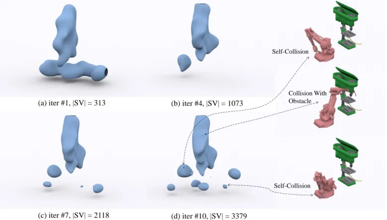
To gain an understanding of our refinement process, a train-ing process is shown in Fig. 3. The blue regions correspond to obstacle regions for the models given on the right. After a few iterations, the approximationCobs finds more isolated obstacle regions.
4. Penetration Depth Computation
In this section, we first define distance metric for articulated models used in our algorithm and then present our approach to compute penetration depth.
4.1. Distance Metric
In this paper, we consider both translational and rotational motion. For an articulated model A, when its configuration changes from q to q0, we use the following displacement to
calculate distance metric [9].
dist(q,q0) =d0+d1+. . .+dn−1, (4)
wheredi is the distance component contributed by jointiand its associated links.
For an articulated model, translational motion is contributed by prismatic joints. When a prismatic joint parameter of Ji
changes fromqitoq0i, the distance contributed by a prismatic joint and its associated linkLi+1is calculated by
di=
Vi+1
V |q
0
i−qi|2, (5)
whereVi+1is the volume ofLi+1andVis the volume ofA.
For a revolute jointJi, the displacement distance by its asso-ciated linkLi+1can be represented as
di= 4
V sin
2
θ
2
ωTi Iiωi, , (6)
whereV is the volume ofA,θis rotation angle calculated by θ=q0i−qi,ωi is the rotational axis of Ji andIi is the inerti-a tensor ofLi+1in reference frame. For a spherical joint, its distance metric can be defined analogously.
4.2. PD Computation Using Discretized∂Cobs
Given an approximation of obstacle regionCobsand a query
q0∈ Cobs, we can compute penetration depth by looking for the nearest point on∂Cobs.
PD(A(q0),O) = min
q∈∂Cobs
dist(q0,q), (7)
whereA(q0)corresponds toAlocated at the configurationq0, PD denotes penetration depth computed using an approximate obstacle regionCobs.
Solving Equation 7 leads to an optimization problem [8, 9]. The solution proposed in [9], depicted in Fig. 4-(a), may lead to a local nearest configurationq2if a random initial guessqgis used. The approach suggested in [8], shown in Fig. 4-(b) uses a nearest support vector as the initial guess and then a constrained optimization is used to search for the closest configuration. The latter may suffer from the problem of slow convergence.
Here, we extend [8] and propose a new approach to perform fast PD computation, described as follows.
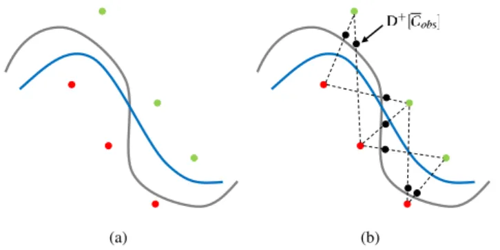
Discretized Representation: A new discretized approxima-tion is generated from the final trained∂Cobs. This will be a discrete representation of∂Cobswith very dense samples. Here, we denote this discretized representation as D[Cobs], where D[Cobs]consists of two components: collision-free configura-tions D+[Cobs] and in-collision configurations D−[Cobs]. This step is illustrated in Fig. 5. To generate a discretized represen-tation, we choose any red in-collision configuration fromSV−
and usek-NN search to find a few green collision-free neigh-bors fromSV+. Then we moveAfrom a green configuration to a red in-collision configuration until a contact is found. This contact corresponds to a configuration near∂Cobs. We add this configuration into D+[Cobs]. As shown in Fig. 5-(b), the black points denote D+[Cobs]after applying our approach. A dotted line depicts a motion trajectory from a green point to a red point. In fact, these trajectories can be very complicated, especially for an articulated model. This step is relatively expensive and is performed in a pre-processing stage afterCobsis obtained.
(a) (b)
Figure 5: Discretized representation model for∂Cobs. (a) Exact boundary of
Cobs(grey) and its approximation using SVM-based machine learning (blue).
Red and green points are support vectors. (b) A discretized representation can be obtained by generating more samples near the exact boundary∂Cobs.
D+[Cobs]represents the collision-free configuration of discretized boundary.
Self-Collision Self-Collision
Collision With Obstacle
(a) iter #1, |SV| = 313 (b) iter #4, |SV| = 1073
(c) iter #7, |SV| = 2118 (d) iter #10, |SV| = 3379
Figure 3: Training process for an articulated model composed of three active revolute joints. (a)∼(d) are four iterations of the learning phase, where|SV|s are the numbers of their support vectors. The images on the right show three different robot poses and their corresponding configurations are highlighted in obstacle regions given in (d).
first quickly determine k1 configurations nearest to the query
configuration q0 for D[Cobs]. For configuration spaces, we use a hierarchical clustering algorithm to perform k-NN search [28]. As shown in Fig. 4-(c), D[Cobs]is depicted using a set of green and red configurations. In our experiment, we choose
k1=50∼100. Then the nearest point is found among thesek1
configurations. As shown in Fig. 4, thesek1-nearest neighbor
configurations are enclosed in eclipses. Then, the closest con-figuration is determined in a brute force manner among thesek1
configurations.
Conservative Penetration Depth: For a given queryq0and the closestq1, ifq1is a collision-free configuration, conserva-tive penetration depth can be readily calculated by dist(q0,q1)
using Equation 4. If q1 is an in-collision configuration, we performk-nearest neighbor algorithm again to findk2
contigu-ous configurations aroundq1. Assume that there exists at least one collision-free configuration among thesek2neighbors, we
search for the nearest oneq1. This process is shown in Figs. 4-(c) and (d). We choosek2=5∼10. An alternative strategy is
to directly search for the nearest neighbor forq0from D+[Cobs]
using the following query.
PD= min
q∈D+[C obs]
dist(q0,q), (8)
qis the closest point in D+[Cobs], see Algorithm 2. Conserva-tive penetration depth and its corresponding configuration can guarantee separating two objects.
5. Results
We implemented our algorithm under the framework of [8], using C++ language. We used Motion Planning Kit [29] for modeling and simulating articulated models and their surround-ing obstacles. We used GraspIt! [30] to perform graspsurround-ing sim-ulation using hand models. We used LIBSVM [31] to perfor-m SVM-based perfor-machine learning. We usedk-nearest neighbor search multiple times. In this section, we test our algorithm us-ing a few simple articulated models. Some complex articulated models will be given in the next section.
5.1. Two-Active-Joint Models
In Fig.1-(a), we show an articulated model and an obstacle. If we only allow two revolute jointsJ0 andJ1to be active, we can obtain their obstacle region shown in Fig.1-(b). We will use this benchmark for comparison between three different pen-etration results (i.e. analytical, approximate and conservative penetration depths).
LetDbe the distance from the first jointJ0to obstacleO. If
0
q
1
q
2
q
g
q
(a)
0
q
1
q
g
q
(b)
0
q
1
q
(c)
0
q
1
q
(d)
Figure 4: Penetration depth query process. (a) A method suggested in [9]. Given a random initial guessqg, an optimization-based algorithm may lead to a local
nearest configurationq2, rather than the global nearest configurationq1. (b) A method suggested in [8]. A nearest support vector serves as the initial guess and then
a constrained optimization is used to search for the closest configuration. (c)-(d) A discrete representation is generated from (b), using similar technique described in Fig. 5. An approximatek-nearest neighbor algorithm may findk1configurations, among which the nearest configuration is identified (denoted by the holly red
pointq1). Finally, the average of all contiguous configurations aroundq1is used to calculate penetration depth.
magnitude of penetration depth is smaller than the exact pen-etration depth. The configuration that realizes this penpen-etration depth does not separate two objects. The conservative penetra-tion depth calculated by our algorithm, shown as a blue curve, is always greater than the exact penetration depth (red).
PD
magnitu
de
Distance
1 1.1 1.2 1.3 1.4 1.5 1.6 1.7 1.8 1.9 2 1.4
1.2
1.0
0.8
0.6
0.4
0.2
0
analytical PD
approximate PD
conservative PD
Figure 6: Analytical, approximate and conservative penetration depths.
Computational Cost: In pre-processing, our algorithm takes nearly 40 seconds for training a binary classifier and obtaining the approximate boundary of obstacle region. There are more than 3000 support vectors in the classifier. It takes additional 293 seconds in pre-processing stage to generate a discretized representation. The runtime query of penetration depth takes 0.047 ms only.
5.2. Self-Colliding Models
In this section, we consider the scenarios with self-collisions. Fig. 7-(a) shows an example of self-collision between two links of an articulated model, where linkL3collides with the base linkL0. If we only allowJ0andJ1to rotate, it is obvious that the exact penetration depth is constant for the query configura-tion shown in Fig. 7-(a). To compare with our results, we first rotateJ0only by a specified angle and compute its conserva-tive penetration depth. The results are shown in 7-(b), where the horizontal axis is the angle of rotation and the vertical axis is the magnitudes of penetration depth .
In addition, we generate different query configurations by ro-tatingJ1. For a query configuration, we compute its conserva-tive penetration depth. WhenL2 and its attached links move from one side ofL0 to the other side, the penetration depth gradually increases and then decreases, as shown in Fig. 7-(c).
0 L
2 L
1
L L3
4 L
0 J
1 J
2 J 3 J
(a) (b)
Figure 8: Self-collision experiment 2. (a) 4-DOF articulated model and self-collision configuration. (b) Penetration depth results for query configurations generated by rotatingJ2.
Fig. 8-(a) shows a more complicated scenario. We let three revolute jointsJ0,J2andJ3 rotate. In order to test our al-gorithm, we start from the configuration shown in Fig. 8-(a) whereL4collide withL2. We rotateJ2to generate some query configurations in a counterclockwise manner. Then we calcu-late penetration depth for these inter-penetration configurations. The results are shown in Fig.8-(b).
Computational Cost: In the first two scenarios, it takes 42 seconds for training approximate obstacle region and 355 sec-onds to generate a discretized representation. It takes 0.058 ms on average for each penetration depth query. In the three dimen-sional scenario, training approximate obstacle region takes 39 seconds and generating a discretized representation takes 138 seconds. Computing penetration depth takes 0.046 ms on aver-age for each query.
5.3. Hybrid Joints
0
L
2
L
1
L
3
L
0
J
1
J
2
J
(a) (b) (c)
Figure 7: Self-collision experiment 1. (a) 3-DOF articulated model and self-collision configuration.J0andJ1are active revolute joints. (b) Only rotatingJ0to
generate query configurations and their corresponding penetration depth. (c) Only rotatingJ1to generate query configurations and their corresponding penetration
depth.
L0andL1 for the articulated model shown in Fig.1-(a). Af-ter adding one degree of freedom, its obstacle region becomes three dimensional space, two dimensions for rotation and one dimension for translation. We generate some query configura-tions by placing obstacleOat different locations. When obsta-cle Omoves away from Aalong horizontal axis, penetration depth magnitude decreases, as shown in Fig. 9. To test the in-fluence of translation component in penetration depth compu-tation, we assign a weight factor to the prismatic joint (refer to Equation 5). Fig.9 shows penetration depth results under three different weights for prismatic joint.
The red line is obtained using the smallest weight. In this case, two objects tend to be separated by translation (prismatic joint) rather than rotation (revolute joints) because it consumes less energy. These penetration depth magnitudes are mainly contributed by translational component and they are smaller than the results given in Fig.6.
The blue line is obtained using the largest translational weight, so rotate joints tend to contribute more in penetration depth computation. In our experiment, the penetration depth magnitudes are similar to those results given in Fig.6.
Distance
PD
Magnit
ude
weight=0.01 weight=0.1 weight=1.0
1.1 1.2 1.3 1.4 1.5 1.6 1.7 1.8 1.9 2.0 1.0
0.2 0.4 0.6 0.8 1.0 1.2 1.4
0.0
Figure 9: Penetration depth for an articulated model with hybrid joints. The prismatic joint is assigned three different weight, ranging from 0.01 to 1.0. The smaller the weight is,the more the translational component contributes.
The green line is for the case using a medium translational weight. When the articulated model and obstacle have a deeper inter-penetration (i.e. larger penetration depth), their penetra-tion depth is determined by both rotapenetra-tion and translapenetra-tion mo-tion. In this case, their penetration depth magnitudes are greater than the translation dominated case (red line), but less than the rotation dominated case (blue line). However, for marginal inter-penetration, a translational component tends to contribute more than a rotational component. The resulting penetration depth tends to be equivalent to the one given in red, as shown in the portion where distance is greater than 1.6.
Computational Cost: In our experiment, it takes 26 seconds to train approximate obstacle region and 68 seconds to generate discretized obstacle region. The average query time for pene-tration depth is 0.03 ms.
6. Complex Articulated Models
In this section, we applied our algorithm to different complex articulated models.
6.1. Benchmarking Scenarios
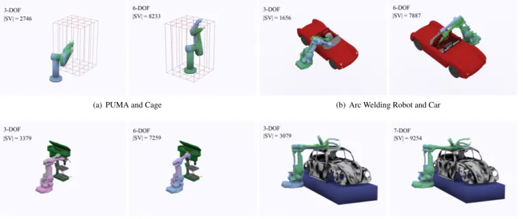
PUMA and Cage: As shown in Fig.10-(a), a PUMA indus-trial robot sweeps into a cage and the two models penetrate each other during the motion. In-collision configurations and collision-free configurations are highlighted in light blue and green, respectively. The PUMA robot consists of 868 triangles and the cage consists of 432 triangles. The left image in Fig.10-(a) shows three active revolute joints. In our experiment, it takes 135 seconds to generate the approximation of obstacle region-s and the number of region-support vectorregion-s|SV|=2746. Computing penetration depth takes 1.09 ms on average per runtime query. For six active joints (shown in the right image of Fig.10-(a)), it takes 350 seconds to generate the approximation of obstacle re-gions and|SV|=8233. It takes 2.25 ms on average to compute penetration depth.
(a) PUMA and Cage (b) Arc Welding Robot and Car
(c) Arc Welding Robot and Drill (d) Spot Welding Robot and Car Body
Figure 10: Conservative penetration depth for high-DOF articulated models. (a)-(c) The benchmarks on the left are 3-DOF experiments and on the right are 6-DOF experiments. (d) The benchmark on the left is a 3-DOF experiment and on the right is a 7-DOF experiment.
collision-free configuration. The arc welding robot consists of 3.7K triangles and the car consists of 19K triangles. In our ex-periment, it takes 117 seconds to generate the approximation of obstacle regions for three active joints. The number of sup-port vectors|SV|=1656. Computing conservative penetration depth takes 0.77 ms. When activating six active joints, it takes 382 seconds to generate the approximation of obstacle regions and 0.85 ms to compute penetration depth.|SV|=7887.
Arc Welding Robot and Drill: As shown in Fig.10-(c), an arc welding industrial robot works beside a drill and the two models penetrate each other during the motion (grey). A collision-free configuration is highlighted in pink. The arc welding robot con-sists of 3.7K triangles and the drill concon-sists of 34K triangles. It takes 62 seconds to generate the approximation of obstacle re-gions for three active joints and|SV|=3379. Computing pen-etration depth takes 0.61 ms. For six active joints, it takes 383 seconds to generate the approximation of obstacle regions and computing penetration depth takes 1.04 ms.|SV|=7259.
Spot Welding Robot and Car Body: As shown in Fig.10-(d), a spot welding industrial robot works around a car body and the two models penetrate each other during the motion (blue). A collision-free configuration is highlighted in green. The spot welding robot consists of 5.6K triangles and the car body con-sists of 4K triangles. The left of Fig.10-(d) is for activating three active joints, it takes 118 seconds to generate the approximation of obstacle regions and |SV|=3079. Computing penetration depth takes 0.62 ms. The right of Fig.10-(d) is for activating seven active joints, it takes 497 seconds to generate the approx-imation of obstacle regions. Computing penetration depth takes 1.91 ms. This scenario is very complex, so it has more support vectors (|SV|=9254) than others.
Hand Grasping: A robot hand grasps a glass (Figs.11). The hand has twelve joints, consisting of 22K triangles. The glass
consists of 3.2K triangles. A sequence of inter-penetration con-figurations are generated during the simulation and our algo-rithm is used to separate two objects. Our algoalgo-rithm takes 403 seconds to generate the approximation of obstacle regions and 1.99 ms to compute penetration depth. |SV|=8245 is fewer than the previous benchmark (spot welding robot and car body), as a glass model is not very complex. Note that we did not take account of any constraint that makes the hand hold the glass.
Motion Planning: We also apply our PD algorithm to a retraction-based probabilistic roadmap (PRM) planner[? ]. We generate some samples in C-space and detect their collision s-tates. If its state is collision-free, the sample will be added in the roadmap. If its state is in-collision, the sample will be used to find a configuration in free space based on our PD algorith-m and a new collision-free configuration will be added in the roadmap. Our PD algorithm can be used to efficiently find these collision-free configurations for given collision configurations. As shown in Fig.12, planning a path for welding robot takes 127 seconds. In total, it generates 20181 samples, among which 3309 samples are computed using our PD algorithm.
6.2. Comparison and Discussion
(a)
(b)
0 0.1 0.2 0.3 0.4 0.5 0.6 0.7 0.8
1 6 11 16 21 26 31 36 41 46 0 0.2 0.4 0.6 0.8 1 1.2 1.4
1 6 11 16 21 26 31 36 41 46
(c)
Figure 11: A 12-DOF robot hand grasps a glass. (a) An inter-penetration con-figuration is shown in two different views; (b) The robot hand and the glass are separated using our algorithm; (c) Conservative PD magnitude and runtime query time.
Fig.14. Both the algorithms achieved similar runtime perfor-mance.
[9] is the only work to approximate penetration depth for ar-ticulated models. Their work uses local contact space projec-tion to iteratively find a local minimum point at the runtime. The query time includes successive perturbation to find start point and iterative contact space projection. Our query time mainly affected by the number of support vectors|SV|. In gen-eral, the runtime query is more efficient than [9] and does not suffer the iterative process. However, we need to spend more time in learning stage than theirs.
6.3. Time Complexity
Learning: The time spent in the learning stage can be esti-mated byT =Tc·Ns+TL+TR+TD , whereTc=Tcol·NL is
(a) (b)
(c) (d)
Figure 12: Screenshots of motion planning using PRM and our PD algorithm.
the time of collision detection (Tcolis collision detection time for one articulated link andNLis the number of links in an ar-ticulated model),Ns is the number of samples,TL is the time to learn an initial approximation,TRis the time for refinemen-t and TD is the time of generating discretized representation.
TD=k·NSV·Tccd, wherekis a number specified by users (i.e.
knearest neighbors with opposite state for a given support vec-tor),NSV is the number of support vectors,Tccd is the time of continuous collision detection for given two configurations.
Query: The time of runtime query is mainly determined by the number of support vectors.
7. Limitations and Conclusions
We presented an efficient algorithm to compute global pen-etration depth for articulated models. The performance gain is due to the use of machine learning techniques and the sim-plification of runtime query. The former dramatically reduces computational complexity and the latter avoids constrained op-timization process. We carried out extensive experiments to demonstrate the efficiency of our algorithm.
Cobs. Applying machine learning techniques and configuration space approximation to these problem would make it possible, especially for high-DOF articulated models. Another direction for future research is to apply our algorithm to motion planning for narrow passages. At the moment, a tight theoretical error bound is not known for the learning algorithm used in our algo-rithm, but evaluating accuracy for specific applications will be another good topic for future work.
Appendix
Below are the pseudocode for training a classifier using SVM to obtain the discretized representation D[Cobs](Algorithm 1) and for computing pPD (Algorithm 2).
In Algorithm 1, a training procedure takes an articulated model A and an obstacleOas input and produces a discrete boundary D[Cobs]. The number of iterations in training refine-ment is governed by argurefine-mentN. Qis a set of configurations obtained in sampling.
Algorithm 1train(A,O,N)
Output: [Discretized Approximation D[Cobs]]
1: Q←sample(A,O)
2: whileN,0do
3: f ←svm(Q)
4: Q←refine(A,O, f,Q)
5: N=N−1
6: end while 7: f ←svm(Q)
8: D[Cobs]←discretized(f,Q)
9: return D[Cobs]
Note that, in step 1, any sampling scheme can be used. In our implementation, we use uniform sampling.
In Algorithm 2, the configuration that realizes PD is deter-mined usingk-nearest neighbor search (denoted by procedure
knn). Q1is a set ofkconfigurations returned by the
approxi-mateknn procedure. The final penetration depth magnitude is calculated using Equations 4, 5 and 6.
Algorithm 2computePD(D[Cobs],q0,k)
Output: [PD magnitude]
1: Q1←knn(D+[Cobs],q0,k) 2: q1←min(Q1)
3: return PD=dist(q0,q1)
[1] L. Zhang, Y. J. Kim, G. Varadhan, D. Manocha, Generalized penetration depth computation, Computer-Aided Design 39 (8) (2007) 625–638. [2] Y. J. Kim, M. C. Lin, D. Manocha, DEEP: Dual-space expansion for
es-timating penetration depth between convex polytopes, in: International Conference on Robotics and Automation, 2002, pp. 921–926.
[3] G. van den Bergen, Proximity queries and penetration depth computation on 3D game objects, in: Game Developers Conference, 2001.
[4] P. K. Agarwal, L. J. Guibas, S. Har-Peled, A. Rabinovitch, M. Sharir, Computing the penetration depth of two convex polytopes in 3d, in: S-candinavian Workshop on Algorithm Theory, 2000, pp. 328–338.
[5] G. Nawratil, H. Pottmann, B. Ravani, Generalized penetration depth com-putation based on kinematical geometry, Computer Aided Geometric De-sign 26 (4) (2009) 425–443.
[6] L. Zhang, Y. J. Kim, D. Manocha, A fast and practical algorithm for gen-eralized penetration depth computation, in: Robotics: Science and Sys-tems, 2007.
[7] C. Je, M. Tang, Y. Lee, M. Lee, Y. J. Kim, Polydepth: Real-time pene-tration depth computation using iterative contact-space projection, ACM Transactions on Graphics. 31 (1) (2012) 5:1–5:14.
[8] J. Pan, X. Zhang, D. Manocha, Efficient penetration depth approximation using active learning, ACM Transactions on Graphics (ACM SIGGRAPH ASIA 2013) 32, article 191.
[9] M. Tang, Y. J. Kim, Interactive generalized penetration depth computation for rigid and articulated models using object norm, ACM Transactions on Graphics 33 (1) (2014) Article No. 1.
[10] X. Zhang, Y. J. Kim, D. Manocha, Continuous penetration depth, Computer-Aided Design 46 (2014) 3–13.
[11] S. Cameron, R. Culley, Determining the minimum translational distance between two convex polyhedra, in: IEEE International Conference on Robotics and Automation, 1986, pp. 591–596, volume 3.
[12] D. Dobkin, J. Hershberger, D. Kirkpatrick, S. Suri, Computing the intersection-depth of polyhedra, Algorithmica 9 (6) (1993) 518–533. [13] S. Cameron, Enhancing GJK: Computing minimum and penetration
dis-tance between convex polyhedra, in: IEEE International Conference on Robotics and Automation, 1997, pp. 3112–3117.
[14] C. J. Ong, E. G. Gilbert, Growth distances: New measures for object sep-aration and penetration, IEEE Transactions on Robotics and Automation 12 (6) (1996) 888–903.
[15] P. Hachenberger, Exact minkowksi sums of polyhedra and exact and effi-cient decomposition of polyhedra into convex pieces, Algorithmica 55 (2) (2009) 329–345.
[16] Y. J. Kim, M. A. Otaduy, M. C. Lin, D. Manocha, Fast pene-tration depth computation for physically-based animation, in: SIG-GRAPH/Eurographics Symposium on Computer Animation, 2002, pp. 23–31.
[17] J.-M. Lien, Covering minkowski sum boundary using points with appli-cations, Computer Aided Geometric Design 25 (8) (2008) 652–666. [18] J.-M. Lien, A simple method for computing minkowski sum boundary
in 3d using collision detection, in: Algorithmic Foundation of Robotics VIII, Vol. 57 of Springer Tracts in Advanced Robotics, Springer Berlin / Heidelberg, 2009, pp. 401–415.
[19] E. Guendelman, R. Bridson, R. Fedkiw, Nonconvex rigid bodies with s-tacking, ACM Transactions on Graphics. 22 (3) (2003) 871–878. [20] S. Redon, M. C. Lin, A fast method for local penetration depth
computa-tion, Graphical Tools 8 (1) (2006) 63–70.
[21] M. Tang, M. Lee, Y. J. Kim, Interactive hausdorff distance computation for general polygonal models, ACM Transactions on Graphics. 28 (3) (2009) 74:1–74:9.
[22] M. Tang, D. Manocha, M. A. Otaduy, R. Tong, Continuous penalty forces, ACM Transactions on Graphics. 31 (4) (2012) 107:1–107:9.
[23] M. Tang, Y. J. Kim, Interactive generalized penetration depth computation for rigid and articulated models using object form, Tech. rep., Department of Computer Science, Ewha Womans University (2012).
[24] B. Wang, F. Faure, D. K. Pai, Adaptive image-based intersection volume, in: SIGGRAPH, 2012, pp. 97:1–9.
[25] B. Heidelberger, M. Teschner, R. Keiser, M. Müller, M. H. Gross, Con-sistent penetration depth estimation for deformable collision response, in: International Fall Workshop on Vision, Modeling and Visualization, 2004, pp. 339–346.
[26] J.-M. Lien, Covering minkowski sum boundary using points with appli-cations, Computer Aided Geometric Design 25 (8) (2008) 652–666. [27] E. Larsen, S. Gottschalk, M. C. Lin, D. Manocha, Fast proximity queries
with swept sphere volumes, in: International Conference on Robotics and Automation, 2000, pp. 3719–3726.
[28] M. Muja, D. G. Lowe, Fast approximate nearest neighbors with auto-matic algorithm configuration, in: International Conference on Computer Vision Theory and Application, 2009, pp. 331–340.
[29] F. Schwarzer, M. Saha, J.-C. Latombe, Motion Planning Kit, http://ai.stanford.edu/∼mitul/mpk/ (2006).
0 0.05 0.1 0.15 0.2
1 11 21 31 41 51
Approximate PD Our Conservative PD
Frame Number PD Magnitud e 0 0.2 0.4 0.6 0.8 1 1.2 1.4
1 11 21 31 41 51
Frame Number
PD Magnitud
e
(a) PUMA and Cage
0 0.001 0.002 0.003 0.004 0.005 0.006 0.007 0.008
1 11 21 31 41 51
Frame Number PD Magnitud e 0 0.02 0.04 0.06 0.08 0.1 0.12
1 11 21 31 41 51
Frame Number
PD Magnitud
e
(b) Arc Welding Robot and Car
0 0.0005 0.001 0.0015 0.002 0.0025 0.003 0.0035 0.004
1 11 21 31 41 51
Frame Number PD Magnitud e 0 0.01 0.02 0.03 0.04 0.05 0.06 0.07 0.08 0.09
1 11 21 31 41 51
Frame Number
PD Ma
gnitu
de
(c) Arc Welding Robot and Drill
0 0.001 0.002 0.003 0.004 0.005 0.006 0.007 0.008 0.009
1 11 21 31 41 51
Frame Number PD Ma gnitu de 0 0.02 0.04 0.06 0.08 0.1 0.12 0.14 0.16 0.18
1 11 21 31 41 51
Frame Number
PD Ma
gnitu
de
(d) Spot Welding Robot and Car Body
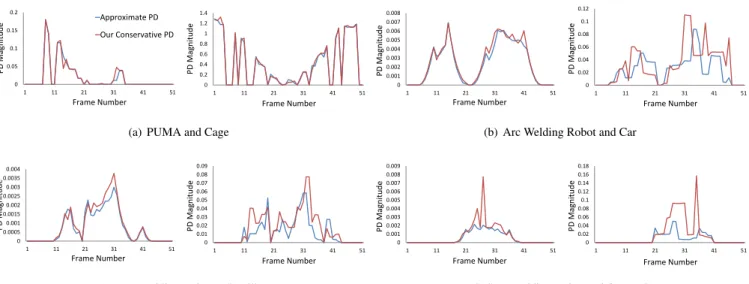
Figure 13: Conservative penetration depth vs approximate penetration depth. Also refer to Fig.10 for corresponding benchmarks.
0 0.5 1 1.5 2
1 11 21 31 41 51
Approximate PD Our Conservative PD
Frame Number time (ms) 0 0.5 1 1.5 2 2.5 3 3.5
1 11 21 31 41 51
Frame Number
time (ms)
(a) PUMA and Cage
0 0.2 0.4 0.6 0.8 1 1.2 1.4 1.6 1.8
1 11 21 31 41 51
Frame Number time (ms) 0 0.5 1 1.5 2 2.5 3
1 11 21 31 41 51
Frame Number
time (ms)
(b) Arc Welding Robot and Drill
0 0.1 0.2 0.3 0.4 0.5 0.6 0.7 0.8 0.9 1
1 11 21 31 41 51
Frame Number time (ms) 0 0.5 1 1.5 2 2.5 3 3.5 4 4.5 5
1 11 21 31 41 51
Frame Number
time (ms)
(c) Arc Welding Robot and Drill
0 0.1 0.2 0.3 0.4 0.5 0.6 0.7 0.8 0.9 1
1 11 21 31 41 51
Frame Number time (ms) 0 1 2 3 4 5 6 7
1 11 21 31 41 51
Frame Number
time (ms)
(d) Spot Welding Robot and Car Body
Figure 14: Computational costs for conservative penetration depth vs approximate penetration depth. Also refer to Fig.10 for corresponding benchmarks.
[31] C.-C. Chang, C.-J. Lin, LIBSVM: A library for support vector ma-chines, ACM Transactions on Intelligent Systems and Technology 2 (2011) 27:1–27:27, software available athttp://www.csie.ntu.

![Figure 4: Penetration depth query process. (a) A method suggested in [9]. Given a random initial guess q g , an optimization-based algorithm may lead to a local nearest configuration q 2 , rather than the global nearest configuration q 1](https://thumb-us.123doks.com/thumbv2/123dok_us/8313316.2202111/6.892.80.826.128.277/penetration-suggested-optimization-algorithm-nearest-configuration-nearest-configuration.webp)