COMPUTING EQUILIBRIA FOR TWO-PERSON GAMES
Appeared as Chapter 45, Handbook of Game Theory with Economic Applications, Vol. 3 (2002), eds. R. J. Aumann and S. Hart, Elsevier, Amsterdam, pages 1723–1759.
BERNHARD VON STENGEL∗ London School of Economics
Contents
1. Introduction 2. Bimatrix games2.1. Preliminaries
2.2. Linear constraints and complementarity 2.3. The Lemke–Howson algorithm
2.4. Representation by polyhedra 2.5. Complementary pivoting 2.6. Degenerate games
2.7. Equilibrium enumeration and other methods 3. Equilibrium refinements
3.1. Simply stable equilibria
3.2. Perfect equilibria and the tracing procedure 4. Extensive form games
4.1. Extensive form and reduced strategic form 4.2. Sequence form
5. Computational issues References
1. Introduction
Finding Nash equilibria of strategic form or extensive form games can be difficult and tedious. A computer program for this task would allow greater detail of game-theoretic models, and enhance their applicability. Algorithms for solving games have been stud-ied since the beginnings of game theory, and have proved useful for other problems in mathematical optimization, like linear complementarity problems.
This paper is a survey and exposition of linear methods for finding Nash equilibria. Above all, these apply to games with two players. In an equilibrium of a two-person game, the mixed strategy probabilities of one player equalize the expected payoffs for the pure strategies used by the other player. This defines an optimization problem with linear constraints. We do not consider nonlinear methods like simplicial subdivision for approximating fixed points, or systems of inequalities for higher-degree polynomials as they arise for noncooperative games with more than two players. These are surveyed in McKelvey and McLennan (1996).
First, we consider two-person games in strategic form (see also Parthasarathy and Raghavan, 1971; Raghavan, 1994, 2002). The classical algorithm by Lemke and Howson (1964) finds one equilibrium of a bimatrix game. It provides an elementary, constructive proof that such a game has an equilibrium, and shows that the number of equilibria is odd, except for degenerate cases. We follow Shapley’s (1974) very intuitive geometric exposition of this algorithm. The maximization over linear payoff functions defines two polyhedra which provide further geometric insight. A complementary pivoting scheme describes the computation algebraically. Then we clarify the notion of degeneracy, which appears in the literature in various forms, most of which are equivalent. The lexico-graphic method extends pivoting algorithms to degenerate games. The problem of finding all equilibria of a bimatrix game can be phrased as a vertex enumeration problem for polytopes.
Second, we look at two methods for finding equilibria of strategic form games with additional refinement properties (see van Damme, 1987, 2002; Hillas and Kohlberg, 2002). Wilson (1992) modifies the Lemke–Howson algorithm for computing simply sta-ble equilibria. These equilibria survive certain perturbations of the game that are easily represented by lexicographic methods for degeneracy resolution. Van den Elzen and Tal-man (1991) present a complementary pivoting method for finding a perfect equilibrium of a bimatrix game.
Third, we review methods for games in extensive form (see Hart, 1992). In princi-ple, such game trees can be solved by converting them to the reduced strategic form and then applying the appropriate algorithms. However, this typically increases the size of the game description and the computation time exponentially, and is therefore infeasible. Approaches to avoiding this problem compute with a small fraction of the pure strategies, which are generated from the game tree as needed (Wilson, 1972; Koller and Megiddo, 1996). A strategic description of an extensive game that does not increase in size is the
sequence form. The central idea, set forth independently by Romanovskii (1962), Selten (1988), Koller and Megiddo (1992), and von Stengel (1996a), is to consider only se-quences of moves instead of pure strategies, which are arbitrary combinations of moves. We will develop the problem of equilibrium computation for the strategic form in a way that can also be applied to the sequence form. In particular, the algorithm by van den Elzen and Talman (1991) for finding a perfect equilibrium carries over to the sequence form (von Stengel, van den Elzen and Talman, 2002).
The concluding section addresses issues of computational complexity, and mentions ongoing implementations of the algorithms.
2. Bimatrix games
We first introduce our notation, and recall notions from polytope theory and linear pro-gramming. Equilibria of a bimatrix game are the solutions to a linear complementarity problem. This problem is solved by the Lemke–Howson algorithm, which we explain in graph-theoretic, geometric, and algebraic terms. Then we consider degenerate games, and review enumeration methods.
2.1. Preliminaries
We use the following notation throughout. Let (A,B) be a bimatrix game, where A and B are m×n matrices of payoffs to the row player 1 and column player 2, respectively. All vectors are column vectors, so an m-vector x is treated as an m×1 matrix. A mixed strategy x for player 1 is a probability distribution on rows, written as an m-vector of probabilities. Similarly, a mixed strategy y for player 2 is an n-vector of probabilities for playing columns. The support of a mixed strategy is the set of pure strategies that have positive probability. A vector or matrix with all components zero is denoted 0. Inequalities like x≥0 between two vectors hold for all components. B> is the matrix B transposed.
Let M be the set of the m pure strategies of player 1 and let N be the set of the n pure strategies of player 2. It is sometimes useful to assume that these sets are disjoint, as in
M={1, . . . ,m}, N={m+1, . . . ,m+n}. (2.1) Then x∈IRM and y∈IRN, which means, in particular, that the components of y are yjfor
j∈N . Similarly, the payoff matrices A and B belong to IRM×N.
Denote the rows of A by ai for i∈M, and the rows of B> by bj for j∈N (so each
b>j is a column of B). Then aiy is the expected payoff to player 1 for the pure strategy i
when player 2 plays the mixed strategy y, and bjx is the expected payoff to player 2 for j
when player 1 plays x.
A best response to the mixed strategy y of player 2 is a mixed strategy x of player 1 that maximizes his expected payoff x>Ay. Similarly, a best response y of player 2 to
x maximizes her expected payoff x>By. A Nash equilibrium is a pair (x,y) of mixed strategies that are best responses to each other. Clearly, a mixed strategy is a best response to an opponent strategy if and only if it only plays pure strategies that are best responses with positive probability:
Theorem 2.1. (Nash, 1951.) The mixed strategy pair (x,y) is a Nash equilibrium of
(A,B) if and only if for all pure strategiesiinM and j inN xi>0 =⇒ aiy=max
k∈M
aky, (2.2)
yj>0 =⇒ bjx=max
k∈N bkx. (2.3)
We recall some notions from the theory of (convex) polytopes (see Ziegler, 1995). An affine combination of points z1, . . . ,zk in some Euclidean space is of the form∑ki=1ziλi
where λ1, . . . ,λk are reals with ∑i=k 1λi=1. It is called a convex combination if λi≥0 for all i. A set of points is convex if it is closed under forming convex combinations. Given points are affinely independent if none of these points is an affine combination of the others. A convex set has dimension d if and only if it has d+1, but no more, affinely independent points.
A polyhedron P in IRd is a set {z∈IRd|Cz≤q}for some matrix C and vector q. It is called full-dimensional if it has dimension d . It is called a polytope if it is bounded. A face of P is a set{z∈P|c>z=q0} for some c∈IRd, q0∈IR so that the inequality c>z≤q0 holds for all z in P. A vertex of P is the unique element of a 0-dimensional face of P. An edge of P is a one-dimensional face of P. A facet of a d -dimensional polyhedron P is a face of dimension d−1. It can be shown that any nonempty face F of P can be obtained by turning some of the inequalities defining P into equalities, which are then called binding inequalities. That is, F={z∈P|ciz=qi, i∈I}, where
ciz≤qi for i∈I are some of the rows in Cz≤q. A facet is characterized by a single
binding inequality which is irredundant, that is, the inequality cannot be omitted without changing the polyhedron (Ziegler, 1995, p. 72). A d -dimensional polyhedron P is called simple if no point belongs to more than d facets of P, which is true if there are no special dependencies between the facet-defining inequalities.
A linear program (LP) is the problem of maximizing a linear function over some polyhedron. The following notation is independent of the considered bimatrix game. Let M and N be finite sets, I⊆ M, J ⊆N , A ∈IRM×N, b∈IRM, c∈IRN. Consider the polyhedron
P={x∈IRN |
∑
j∈N
ai jxj=bi, i∈M−I,
∑
j∈N
ai jxj≤bi, i∈I,
Any x belonging to P is called primal feasible. The primal LP is the problem
maximize c>x subject to x∈P. (2.4) The corresponding dual LP has the feasible set
D={y∈IRM |
∑
i∈M
yiai j =cj, j∈N−J,
∑
i∈M
yiai j ≥cj, j∈J,
yi≥0, i∈I}
and is the problem
minimize y>b subject to y∈D. (2.5) Here the indices in I denote primal inequalities and corresponding nonnegative dual vari-ables, whereas those in M−I denote primal equality constraints and corresponding un-constrained dual variables. The sets J and N−J play the same role with “primal” and “dual” interchanged. By reversing signs, the dual of the dual LP is again the primal. We recall the duality theorem of linear programming, which states (a) that for any primal and dual feasible solutions, the corresponding objective functions are mutual bounds, and (b) if the primal and the dual LP both have feasible solutions, then they have optimal solutions with the same value of their objective functions.
Theorem 2.2. Consider the primal-dual pair of LPs (2.4), (2.5). Then
(a) (Weak duality.) c>x≤y>bfor all x∈Pandy∈D.
(b) (Strong duality.) If P6=Ø andD6=Øthenc>x=y>bfor some x∈Pandy∈D.
For a proof see Schrijver (1986). As an introduction to linear programming we recommend Chv´atal (1983).
2.2. Linear constraints and complementarity
Mixed strategies x and y of the two players are nonnegative vectors whose components sum up to one. These are linear constraints, which we define using
E = [1, . . . ,1]∈IR1×M, e=1, F= [1, . . . ,1]∈IR1×N, f =1. (2.6) Then the sets X and Y of mixed strategies are
X ={x∈IRM|Ex=e, x≥0}, Y ={y∈IRN|Fy= f, y≥0}. (2.7)
With the extra notation in (2.6), the following considerations apply also if X and Y are more general polyhedra, where Ex=e and Fy= f may consist of more than a single row of equations. Such polyhedrally constrained games, first studied by Charnes (1953) for the zero-sum case, are useful for finding equilibria of extensive games (see Section 4).
Given a fixed y in Y , a best response of player 1 to y is a vector x in X that maximizes the expression x>(Ay). That is, x is a solution to the LP
maximize x>(Ay) subject to Ex=e, x≥0. (2.8)
The dual of this LP with variables u (by (2.6) only a single variable) states minimize
u e
>
u subject to E>u≥Ay. (2.9) Both LPs are feasible. By Theorem 2.2(b), they have the same optimal value.
Consider now a zero-sum game, where B=−A. Player 2, when choosing y, has to assume that her opponent plays rationally and maximizes x>Ay. This maximum payoff to player 1 is the optimal value of the LP (2.8), which is equal to the optimal value e>u of the dual LP (2.9). Player 2 is interested in minimizing e>u by her choice of y. The constraints of (2.9) are linear in u and y even if y is treated as a variable, which must belong to Y . So a minmax strategy y of player 2 (minimizing the maximum amount she has to pay) is a solution to the LP
minimize
u,y e
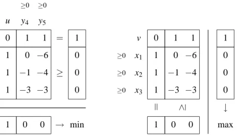
>u subject to Fy= f, E>u−Ay≥0, y≥0. (2.10) Figure 2.1 shows an example.
u y4 y5 ≥0 ≥0
1 1 1
0
−1
−3
−6
−4
−3
0 1 1
1 0 0
0 0 0 1
≥ =
→ min
v x1 x2 x3 ≥0 ≥0 ≥0
1 1 1
0
−1
−3
−6
−4
−3
0 1 1
1 0 0
0 0 0 1
∧ ↓
max
Figure 2.1. Left: Example of the LP (2.10) for a 3×2 zero-sum game. The objective function is separated by a line, nonnegative variables are marked by “≥0”. Right: The dual LP (2.11), to be read vertically.
The dual of the LP (2.10) has variables v and x corresponding to the primal con-straints Fy= f and E>u−Ay≥0, respectively. It has the form
maximize f>v subject to Ex=e, F>v−A>x≤0, x≥0. (2.11)
It is easy to verify that this LP describes the problem of finding a maxmin strategy x (with maxmin payoff f>v) for player 1. We have shown the following.
Theorem 2.3. A zero-sum game with payoff matrix A for player 1 has the equilibrium
(x,y) if and only if u,y is an optimal solution to the LP (2.10) and v,x is an optimal solution to its dual LP (2.11). Thereby,e>u is the maxmin payoff to player 1 and f>vis the minmax payoff to player 2. Both payoffs are equal and denote the value of the game.
Thus, the “maxmin = minmax” theorem for zero-sum games follows directly from LP duality (see also Raghavan, 1994). This connection was noted by von Neumann and Dantzig in the late 1940s when linear programming took its shape. Conversely, linear programs can be expressed as zero-sum games (see Dantzig, 1963, p. 277). There are standard algorithms for solving LPs, in particular Dantzig’s Simplex algorithm. Usually, they compute a primal solution together with a dual solution which proves that the opti-mum is reached.
A best response x of player 1 against the mixed strategy y of player 2 is a solution to the LP (2.8). This is also useful for games that are not zero-sum. By strong duality, a feasible solution x is optimal if and only if there is a dual solution u fulfilling E>u≥Ay and x>(Ay) =e>u, that is, x>(Ay) = (x>E>)u or equivalently
x>(E>u−Ay) =0. (2.12) Because the vectors x and E>u−Ay are nonnegative, (2.12) states that they have to be complementary in the sense that they cannot both have positive components in the same position. This characterization of an optimal primal-dual pair of feasible solutions is known as complementary slackness in linear programming. Since x has at least one pos-itive component, the respective component of E>u−Ay is zero and u is by (2.6) the maximum of the components of Ay. Any pure strategy i in M of player 1 is a best re-sponse to y if and only if the ith component of the slack vector E>u−Ay is zero. That is, (2.12) is equivalent to (2.2).
For player 2, strategy y is a best response to x if and only if it maximizes (x>B)y subject to y∈Y . The dual of this LP is the following LP analogous to (2.9): minimize f>v subject to F>v≥B>x. Here, a primal-dual pair y,v of feasible solutions is optimal if and only if, analogous to (2.12),
y>(F>v−B>x) =0. (2.13) Considering these conditions for both players, this shows the following.
Theorem 2.4. The game(A,B)has the Nash equilibrium(x,y)if and only if for suitable
u,v
Ex =e
Fy= f E>u −Ay≥0
F>v−B>x ≥0
x, y≥0
and (2.12), (2.13) hold.
The conditions in Theorem 2.4 define a so-called mixed linear complementarity problem (LCP). There are various solutions methods for LCPs. For a comprehensive treatment see Cottle, Pang, and Stone (1992). The most important method for finding one solution of the LCP in Theorem 2.4 is the Lemke–Howson algorithm.
2.3. The Lemke–Howson algorithm
In their seminal paper, Lemke and Howson (1964) describe an algorithm for finding one equilibrium of a bimatrix game. We follow Shapley’s (1974) exposition of this algorithm. It requires disjoint pure strategy sets M and N of the two players as in (2.1). Any mixed strategy x in X and y in Y is labeled with certain elements of M∪N . These labels denote the unplayed pure strategies of the player and the pure best responses of his or her opponent. For i∈M and j∈N , let
X(i) ={x∈X|xi=0},
X(j) ={x∈X|bjx≥bkx for all k∈N},
Y(i) ={y∈Y |aiy≥aky for all k∈M},
Y(j) ={y∈Y |yj=0}.
Then x has label k if x∈X(k)and y has label k if y∈Y(k), for k∈M∪N . Clearly, the best-response regions X(j)for j∈N are polytopes whose union is X . Similarly, Y is the union of the sets Y(i) for i∈M. Then a Nash equilibrium is a completely labeled pair
(x,y) since then by Theorem 2.1, any pure strategy k of a player is either a best response or played with probability zero, so it appears as a label of x or y.
Theorem 2.5. A mixed strategy pair (x,y) in X×Y is a Nash equilibrium of (A,B) if and only if for allk∈M∪N eitherx∈X(k)or y∈Y(k)(or both).
For the 3×2 bimatrix game(A,B)with
A=
02 65
3 3
, B= 10 02
4 3
, (2.15)
the labels of X and Y are shown in Figure 2.2. The equilibria are(x1,y1) =
³
(0,0,1)>,(1,0)>
´
where x1has the labels 1, 2, 4 (and y1the remaining labels 3 and 5),(x2,y2) =
³ (0,1
3, 2 3)>,(
2 3,
1 3)>
´
with labels 1, 4, 5 for x2, and(x3,y3) =
³ (2
3, 1 3,0)
>,(1 3,
2 3)
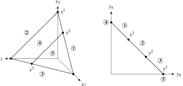
>´with labels 3, 4, 5 for x3. This geometric-qualitative inspection is very suitable for finding equilibria of games of up to size 3×3. It works by inspecting any point x in X with m labels and checking if there is a point y in Y having the remaining n labels. Usually, any x in X has at most m labels, and any y in Y has at most n labels. A game with this property is called nondegenerate, as stated in the following equivalent definition.
@ @ @ @ @ x1 x2 x3 x1 x2 x3 ¾ R 6 ¡¡ ¡¡ ¡¡ ¡¡ ¡¡ ¡ ¡¡ ¡¡ ¡¡ ¡ XXXX XXXX
XXXXXXCCC C C C C C C C C C C C • • • • • °1 °3 °2 °4 °5 y5 y4 -6 @ @ @ @ @ @ @ @ @ @ @@• • • • °1 °2 °3 °5 °4 y3 y2 y1
Figure 2.2. Mixed strategy sets X and Y of the players for the bimatrix game (A,B) in (2.15). The labels 1,2,3, drawn as circled numbers, are the pure strategies of player 1 and marked in X where they have probability zero, in Y where they are best responses. The pure strategies of player 2 are similar labels 4,5. The dots mark points x and y with a maximum number of labels.
Definition 2.6. A bimatrix game is callednondegenerate if the number of pure best re-sponses to a mixed strategy never exceeds the size of its support.
A game is usually nondegenerate since every additional label introduces an equation that reduces the dimension of the set of points having these labels by one. Then only single points x in X have m given labels and single points y in Y have n given labels, and no point has more labels. Nondegeneracy is discussed in greater detail in Section 2.6 below. Until further notice, we assume that the game is nondegenerate.
Theorem 2.7. In a nondegeneratem×nbimatrix game (A,B), only finitely many points inX havemlabels and only finitely many points inY havenlabels.
Proof. Let K and L be subsets of M∪N with|K|=m and|L|=n. There are only finitely many such sets. Consider the set of points in X having the labels in K , and the set of points in Y having the labels in L. By Theorem 2.10(c) below, these sets are empty or singletons.
The finitely many points in the preceding theorem are used to define two graphs G1 and G2. Let G1 be the graph whose vertices are those points x in X that have m labels, with an additional vertex 0 in IRM that has all labels i in M. Any two such vertices x and x0 are joined by an edge if they differ in one label, that is, if they have m−1 labels in common. Similarly, let G2 be the graph with vertices y in Y that have n labels, with the extra vertex 0 in IRN having all labels j in N , and edges joining those vertices that have n−1 labels in common. The product graph G1×G2 of G1 and G2 has vertices (x,y)
where x is a vertex of G1, and y is a vertex of G2. Its edges are given by{x} × {y,y0}for vertices x of G1 and edges{y,y0} of G2, or by{x,x0} × {y} for edges{x,x0} of G1 and vertices y of G2.
The Lemke–Howson algorithm can be defined combinatorially in terms of these graphs. Let k∈ M∪N , and call a vertex pair (x,y) of G1×G2 k-almost completely labeled if any l in M∪N− {k}is either a label of x or of y. Since two adjacent vertices x,x0 in G1, say, have m−1 labels in common, the edge {x,x0} × {y}of G1×G2 is also called k-almost completely labeled if y has the remaining n labels except k. The same applies to edges{x} × {y,y0}of G1×G2.
Then any equilibrium (x,y)is in G1×G2 adjacent to exactly one vertex pair (x0,y0) that is k-almost completely labeled: Namely, if k is the label of x, then x is joined to the vertex x0 in G1 sharing the remaining m−1 labels, and y=y0. If k is the label of y, then y is similarly joined to y0 in G2 and x=x0. In the same manner, a k-almost completely labeled pair(x,y)that is completely labeled has exactly two neighbors in G1×G2. These are obtained by dropping the unique duplicate label that x and y have in common, joining to an adjacent vertex either in G1 and keeping y fixed, or in G2 and keeping x fixed. This defines a unique k-almost completely labeled path in G1×G2connecting one equilibrium to another. The algorithm is started from the artificial equilibrium(0,0)that has all labels, follows the path where label k is missing, and terminates at a Nash equilibrium of the game. ´´ ´´ ´´ ´´ ´´ ´´ ´´ ´´ ´´ ´´ ³³³³ ³³³³ ³³ • 0 ¡¡ ¡¡ ¡¡ ¡¡ ¡¡ ¡¡ ¡¡ ¡¡¡ XXXX XXXX
XXXXXCCC C C C C C C C C C C • •y • • W -• °1 °1 °3 °2 °4
°5 I III V x1 x2 x3 6 @ @ @ @ @ @ @ @ @ @ @@ • • • R• • I °1 °2 °3 °5 °4 0 y3 y2 y1 II IV VI
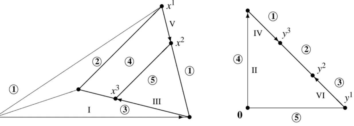
Figure 2.3. The graphs G1and G2for the game in (2.15). The set of 2-almost completely labeled pairs is formed by the paths with edges (in G1×G2) I–II–III–IV, connecting the artificial equilibrium(0,0)and(x3,y3), and V–VI, connecting the equilibria(x1,y1)and(x2,y2).
Figure 2.3 demonstrates this method for the above example. Let 2 be the missing label k. The algorithm starts with x= (0,0,0)> and y= (0,0)>. Step I: y stays fixed and x is changed in G1 to (0,1,0)>, picking up label 5, which is now duplicate. Step II: dropping label 5 in G2changes y to(0,1)>, picking up label 1. Step III: dropping label 1
in G1 changes x to x3, picking up label 4. Step IV: dropping label 4 in G2 changes y to y3 which has the missing label 2, terminating at the equilibrium (x3,y3). In a similar way, steps V and VI indicated in Figure 2.3 join the equilibria(x1,y1) and (x2,y2) on a 2-almost completely labeled path. In general, one can show the following.
Theorem 2.8. (Lemke and Howson, 1964; Shapley, 1974.) Let(A,B)be a nondegenerate bimatrix game and k be a label in M∪N. Then the set of k-almost completely labeled vertices and edges inG1×G2 consists of disjoint paths and cycles. The endpoints of the
paths are the equilibria of the game and the artificial equilibrium (0,0). The number of Nash equilibria of the game is odd.
This theorem provides a constructive, elementary proof that every nondegenerate game has an equilibrium, independently of the result of Nash (1951). By different labels k that are dropped initially, it may be possible to find different equilibria. However, this does not necessarily generate all equilibria, that is, the union of the k-almost completely labeled paths in Theorem 2.8 for all k∈M∪N may be disconnected (Shapley, 1974, p. 183, reports an example due to R. Wilson). For similar observations see Aggarwal (1973), Bastian (1976), Todd (1976, 1978). Shapley (1981) discusses more general methods as a potential way to overcome this problem.
2.4. Representation by polyhedra
The vertices and edges of the graphs G1 and G2 used in the definition of the Lemke– Howson algorithm can be represented as vertices and edges of certain polyhedra. Let
H1={(x,v)∈IRM×IR|x∈X, B>x≤F>v}, H2={(y,u)∈IRN×IR|y∈Y, Ay≤E>u}.
(2.16)
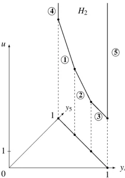
The elements of H1×H2 represent the solutions to (2.14). Figure 2.4 shows H2 for the example (2.15). The horizontal plane contains Y as a subset. The scalar u, drawn vertically, is at least the maximum of the functions aiy for the rows ai of A and for y
in Y . The maximum itself shows which strategy of player 1 is a best response to y. Consequently, projecting H2 to Y by mapping (y,u) to y, in Figure 2.4 shown as (y,0), reveals the subdivision of Y into best-response regions Y(i) for i∈M as in Figure 2.2. Figure 2.4 shows also that the unbounded facets of H2 project to the subsets Y(j) of Y for j∈N . Furthermore, the maximally labeled points in Y marked by dots appear as projections of the vertices of H2. Similarly, the facets of H1 project to the subsets X(k) of X for k∈M∪N .
The graph structure of H1 and H2 with its vertices and edges is therefore identical to that of G1 and G2, except for the m unbounded edges of H1 and the n unbounded edges of H2 that connect to “infinity” rather than to the additional vertex 0 of G1 and G2, respectively.
¡¡ ¡¡
¡¡ ¡¡
-6
µ
y4
0 1
1 u
1
y5
H2
B B
B B
B B
B A
A A
AA
@ @ @
r r r r
@ @ @ @ @ @ @
°4
°1
°2 °3
°5
r r r r
Figure 2.4. The polyhedron H2for the game in (2.15), and its projection to the set{(y,0)| (y,u)∈H2}. The vertical scale is displayed shorter. The circled numbers label the facets of H2 analogous to Figure 2.2.
The constraints (2.14) defining H1 and H2 can be simplified by eliminating the pay-off variables u and v, which works if these are always positive. For that purpose, assume that
A and B> are nonnegative and have no zero column. (2.17) This assumption can be made without loss of generality since a constant can be added to all payoffs without changing the game in a material way, so that, for example, A>0 and
B>0. For examples like (2.15), zero matrix entries are also admitted in (2.17). By (2.6),
u and v are scalars and E> and F> are single columns with all components equal to one, which we denote by the vectors 1M in IRM and 1N in IRN, respectively. Let
P1={x0∈IRM |x0≥0, B>x0≤1N}, P2={y0∈IRN |Ay0≤1M, y0≥0}.
(2.18)
It is easy to see that (2.17) implies that P1 and P2 are full-dimensional polytopes, unlike H1 and H2.
The set H1 is in one-to-one correspondence with P1− {0} with the map (x,v)7→ x·(1/v). Similarly, (y,u)7→y·(1/u) defines a bijection H2 →P2− {0}. These maps have the respective inverse functions x07→(x,v)and y07→(y,u)with
These bijections are not linear. However, they preserve the face incidences since a binding inequality in H1 corresponds to a binding inequality in P1 and vice versa. In particular, vertices have the same labels defined by the binding inequalities, which are some of the m+n inequalities defining P1and P2 in (2.18).
. r -6
0 y0j yj
0 1 u ¡¡ ¡ -6 µ ©©©© ©©©© ©©©© ©© ### ## ## ## ## £££ ££ ££ ££ ££ ££ ££ ££ ££ ££ P2 H2 y4 0 1 u y5
¡¡. .XX........
B B B B B B B A A A AA @ @ @ r r r r @ @ @ @ @ @ @ . . .
Figure 2.5. The map H2→P2, (y,u)7→y0=y·(1/u)as a projective transformation with projection point(0,0). The left-hand side shows this for a single component yj of y, the right-hand side shows how P2 arises in this way from H2 in the example (2.15).
Figure 2.5 shows a geometric interpretation of the bijection (y,u)7→ y·(1/u) as a projective transformation (see Ziegler, 1995, Sect. 2.6). On the left-hand side, the pair
(yj,u)is shown as part of(y,u)in H2for any component yjof y. The line connecting this
pair to(0,0)contains the point(y0j,1)with y0j=yj/u. Thus, P2×{1}is the intersection of the lines connecting any(y,u)in H2with(0,0)in IRN×IR with the set{(y0,1)|y0∈IRN}. The vertices 0 of P1and P2do not arise as such projections, but correspond to H1and H2 “at infinity”.
2.5. Complementary pivoting
Traversing a polyhedron along its edges has a simple algebraic implementation known as pivoting. The constraints defining the polyhedron are thereby represented as linear equations with nonnegative variables. For P1×P2, these have the form
Ay0+r =1M
B>x0 +s=1N
with x0,y0,r,s≥0 where r∈IRM and s∈IRN are vectors of slack variables. The system (2.20) is of the form
Cz=q (2.21)
for a matrix C, right-hand side q, and a vector z of nonnegative variables. The matrix C has full rank, so that q belongs always to the space spanned by the columns Cj of C. A
basis β is given by a basis {Cj | j∈β} of this column space, so that the square matrix
Cβ formed by these columns is invertible. The corresponding basic solution is the unique vector zβ = (zj)j∈β with Cβzβ =q, where the variables zj for j in β are called basic
variables, and zj =0 for all nonbasic variables zj, j 6∈β, so that (2.21) holds. If this
solution fulfills also z≥0, then the basis β is called feasible. If β is a basis for (2.21), then the corresponding basic solution can be read directly from the equivalent system Cβ−1Cz=Cβ−1q, called a tableau, since the columns of C−β1C for the basic variables form the identity matrix. The tableau and thus (2.21) is equivalent to the system
zβ =Cβ−1q−
∑
j6∈β
Cβ−1Cjzj (2.22)
which shows how the basic variables depend on the nonbasic variables.
Pivoting is a change of the basis where a nonbasic variable zj for some j not in β
enters and a basic variable zi for some i in β leaves the set of basic variables. The pivot
step is possible if and only if the coefficient of zj in the ith row of the current tableau is
nonzero, and is performed by solving the ith equation for zj and then replacing zj by the
resulting expression in each of the remaining equations.
For a given entering variable zj, the leaving variable is chosen to preserve feasibility
of the basis. Let the components of Cβ−1q be qi and of Cβ−1Cj be ci j, for i∈β. Then the
largest value of zj such that in (2.22), zβ =Cβ−1q−C−β1Cjzj is nonnegative is obviously
given by
min{qi/ci j |i∈β, ci j >0}. (2.23)
This is called a minimum ratio test. Except in degenerate cases (see below), the minimum in (2.23) is unique and determines the leaving variable zi uniquely. After pivoting, the
new basis isβ∪ {j} − {i}.
The choice of the entering variable depends on the solution that one wants to find. The Simplex method for linear programming is defined by pivoting with an entering vari-able that improves the value of the objective function. In the system (2.20), one looks for a complementary solution where
x0>r=0, y0>s=0 (2.24) because it implies with (2.19) the complementarity conditions (2.12) and (2.13) so that
variable has value zero and represents a binding inequality, that is, a facet of the poly-tope. Hence, each basis defines a vertex which is labeled with the indices of the nonbasic variables. The variables of the system come in complementary pairs (xi,ri) for the
in-dices i∈M and(yj,sj) for j∈N . Recall that the Lemke–Howson algorithm follows a
path of solutions that have all labels in M∪N except for a missing label k. Thus a k-almost completely labeled vertex is a basis that has exactly one basic variable from each complementary pair, except for a pair of variables (xk,rk), say (if k∈M) that are both
basic. Correspondingly, there is another pair of complementary variables that are both nonbasic, representing the duplicate label. One of them is chosen as the entering variable, depending on the direction of the computed path. The two possibilities represent the two k-almost completely labeled edges incident to that vertex. The algorithm is started with all components of r and s as basic variables and nonbasic variables(x0,y0) = (0,0). This initial solution fulfills (2.24) and represents the artificial equilibrium.
Algorithm 2.9. (Complementary pivoting.) For a bimatrix game (A,B)fulfilling (2.17), compute a sequence of basic feasible solutions to the system (2.20) as follows.
(a) Initialize with basic variables r=1M, s=1N. Choose k∈M∪N, and let the first
entering variable be x0k ifk∈M andy0k ifk∈N.
(b) Pivot such as to maintain feasibility using the minimum ratio test.
(c) If the variable zi that has just left the basis has indexk, stop. Then (2.24) holds and (x,y) defined by (2.19) is a Nash equilibrium. Otherwise, choose the complement of zias the next entering variable and go to(b).
We demonstrate Algorithm 2.9 for the example (2.15). The initial basic solution in the form (2.22) is given by
r1=1 −6y05 r2=1−2y04−5y05 r3=1−3y04−3y05
(2.25)
and
s4=1−x01 −4x03 s5=1 −2x02−3x03.
(2.26)
Pivoting can be performed separately for these two systems since they have no variables in common. With the missing label 2 as in Figure 2.3, the first entering variable is x02. Then the second equation of (2.26) is rewritten as x02= 12−32x03−12s5 and s5 leaves the basis. Next, the complement y05of s5enters the basis. The minimum ratio (2.23) in (2.25) is 1/6, so that r1 leaves the basis and (2.25) is replaced by the system
y05= 16 −16r1 r2= 16−2y04+56r1 r3= 12−3y04+12r1.
Then the complement x01of r1 enters the basis and s4leaves, so that the system replacing (2.26) is now
x01=1−4x03−s4
x02=12−32x03 −12s5.
(2.28)
With y04 entering, the minimum ratio (2.23) in (2.27) is 1/12, where r2 leaves the basis and (2.27) is replaced by
y05= 16− 16r1 y04= 121 +125r1−12r2 r3= 14− 34r1+32r2.
(2.29)
Then the algorithm terminates since the variable r2, with the missing label 2 as index, has become nonbasic. The solution defined by the final systems (2.28) and (2.29), with the nonbasic variables on the right-hand side equal to zero, fulfills (2.24). Renormalizing x0 and y0 by (2.19) as probability vectors gives the equilibrium (x,y) = (x3,y3) mentioned after (2.15) with payoffs 4 to player 1 and 2/3 to player 2.
Assumption (2.17) with the simple initial basis for the system (2.20) is used by Wilson (1992). Lemke and Howson (1964) assume A<0 and B<0, so that P1 and P2 are unbounded polyhedra and the almost completely labeled path starts at the vertex at the end of an unbounded edge. To avoid the renormalization (2.19), the Lemke–Howson algorithm can also be applied to the system (2.14) represented in equality form. Then the unconstrained variables u and v have no slack variables as counterparts and are always basic, so they never leave the basis and are disregarded in the minimum ratio test. Then the computation has the following economic interpretation (Wilson, 1992; van den Elzen, 1993): Let the missing label k belong to M. Then the basic slack variable rk which is
basic together with xk can be interpreted as a “subsidy” payoff for the pure strategy k
so that player 1 is in equilibrium. The algorithm terminates when that subsidy or the probability xk vanishes. Player 2 is in equilibrium throughout the computation.
2.6. Degenerate games
The path computed by the Lemke–Howson algorithm is unique only if the game is nonde-generate. Like other pivoting methods, the algorithm can be extended to degenerate games by “lexicographic perturbation”, as suggested by Lemke and Howson (1964). Before we explain this, we show that various definitions of nondegeneracy used in the literature are equivalent. In the following theorem, IM denotes the identity matrix in IRM×M.
Further-more, a pure strategy i of player 1 is called payoff equivalent to a mixed strategy x of player 1 if it produces the same payoffs, that is, ai=x>A. The strategy i is called weakly
dominated by x if ai≤x>A, and strictly dominated by x if ai<x>A holds. The same
applies to the strategies of player 2.
Theorem 2.10. Let (A,B) be an m×n bimatrix game so that (2.17) holds. Then the following are equivalent.
(a) The game is nondegenerate according to Definition 2.6.
(b) For any x in X and y inY, the rows of
·
IM
B>
¸
for the labels of x are linearly inde-pendent, and the rows of
·
A IN
¸
for the labels ofy are linearly independent.
(c) For anyxinX with set of labelsK andyinY with set of labelsL, the setTk∈KX(k)
has dimension m− |K|, and the setTl∈LY(l) has dimensionn− |L|.
(d) P1 and P2 in (2.18) are simple polytopes, and any pure strategy of a player that
is weakly dominated by or payoff equivalent to another mixed strategy is strictly dominated by some mixed strategy.
(e) In any basic feasible solution to (2.20), all basic variables have positive values.
Lemke and Howson (1964) define nondegenerate games by condition (b). Krohn et al. (1991), and, in slightly weaker form, Shapley (1974), define nondegeneracy as in (c). Van Damme (1987, p. 52) has observed the implication (b)⇒(a). Some of the implications between the conditions (a)–(e) in Theorem 2.10 are easy to prove, whereas others require more work. For details of the proof see von Stengel (1996b).
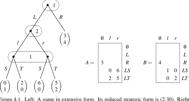
The m+n rows of the matrices in (b) define the inequalities for the polytopes P1and P2 in (2.18), where the labels denote binding inequalities. This condition explains why a generic bimatrix game is nondegenerate with probability one: We call a game generic if each payoff is drawn randomly and independently from a continuous distribution, for example the normal distribution with small variance around an approximate value for the respective payoff. Then the rows of the matrices described in 2.10(b) are linearly independent with probability one, since a linear dependence imposes an equation on at least one payoff, which is fulfilled with probability zero. However, the strategic form of an extensive game (like Figure 4.1 below) is often degenerate since its payoff entries are not independent. A systematic treatment of degeneracy is therefore of interest.
The dimensionality condition in Theorem 2.10(c) has been explained informally before Theorem 2.7 above. The geometric interpretation of nondegeneracy in 2.10(d) consists of two parts. The polytope P1 (and similarly P2) is simple since a point that belongs to more than m facets of P1 has too many labels. In the game
A=
02 65
3 3
, B= 10 02
4 4
, (2.30)
the polytope P1 is not simple because its vertex (0,0,14)> belongs to four facets. This game is degenerate since the pure strategy 3 of player 1 has two best responses. Apart from this, degeneracy may result due to a redundancy of the description of the polytope by inequalities (for example, if A has two identical rows of payoffs to player 1). It is not hard to show that such redundant inequalities correspond to weakly dominated strategies.
A binding inequality of this sort defines a face of the respective polytope. The strict dominance in (d) asserts that this face is empty if the game is nondegenerate.
Theorem 2.10(e) states that every feasible basis of the system is nondegenerate, that is, all basic variables have positive values. This condition implies that the leaving variable in step (b) of Algorithm 2.9 is unique, since otherwise, another variable that could also leave the basis but stays basic will have value zero after the pivoting step. This concludes our remarks on Theorem 2.10.
The lexicographic method extends the minimum ratio test in such a way that the leaving variable is always unique, even in degenerate cases. The method simulates an infinitesimal perturbation of the right-hand side of the given linear system (2.21), z≥0,
and works as follows. Let Q be a matrix of full row rank with k columns. For anyε≥0, consider the system
Cz=q+Q·(ε1, . . . ,εk)> (2.31) which is equal to (2.21) forε =0 and which is a perturbed system forε>0. Let β be a basis for this system with basic solution
zβ =Cβ−1q+Cβ−1Q·(ε1, . . . ,εk)>=q+Q·(ε1, . . . ,εk)> (2.32) and zj=0 for j6∈β. It is easy to see that zβ is positive for all sufficiently smallε if and
only if all rows of the matrix[q,Q]are lexico-positive, that is, the first nonzero component of each row is positive. Thenβ is called a lexico-feasible basis. This holds in particular for q>0 when β is a nondegenerate basis for the unperturbed system. Because Q has full row rank, Q has no zero row, which implies that any feasible basis for the perturbed system is nondegenerate.
In consequence, the leaving variable for the perturbed system is always unique. It is determined by the following lexico-minimum ratio test. Like for the minimum ratio test (2.23), let, for i∈β, the entries of the entering column Cβ−1Cj be ci j, those of q in (2.32)
be qi0, and those of Q be qil for 1≤l≤k. Then the leaving variable is determined by the maximum choice of the entering variable zj such that all basic variables zi in (2.31) stay
nonnegative, that is,
zi=qi0+qi1ε1+· · ·+qikεk−ci jzj≥0
for all i∈β. For sufficiently small ε, the sharpest bound for zj is obtained for that i in
β with the lexicographically smallest row vector 1/ci j·(qi0,qi1, . . . ,qik) where ci j >0
(a vector is called lexicographically smaller than another if it is smaller in the first com-ponent where the vectors differ). No two of these row vectors are equal since Q has full row rank. Therefore, this lexico-minimum ratio test, which extends (2.23), deter-mines the leaving variable zi uniquely. By construction, it preserves the invariant that all
computed bases are lexico-feasible, provided this holds for the initial basis like that in Al-gorithm 2.9(a) which is nondegenerate. Since the computed sequence of bases is unique, the computation cannot cycle and terminates like in the nondegenerate case.
The lexico-minimum ratio test can be performed without actually perturbing the system, since it only depends on the current basis β and Q in (2.32). The actual values of the basic variables are given by q, which may have zero entries, so the perturbation applies as ifε is vanishing. The lexicographic method requires little extra work (and none for a nondegenerate game) since Q can be equal to C or to that part of C containing the identity matrix, so that Q in (2.32) is just the respective part of the current tableau. Wilson (1992) uses this to compute equilibria with additional stability properties, as discussed in Section 3.1 below. Eaves (1971) describes a general setup of lexicographic systems for LCPs and shows various ways (pp. 625, 629, 632) of solving bimatrix games with Lemke’s algorithm (Lemke, 1965), a generalization of the Lemke–Howson method.
2.7. Equilibrium enumeration and other methods
For a given bimatrix game, the Lemke–Howson algorithm finds at least one equilibrium. Sometimes, one wishes to find all equilibria, for example in order to know if an equilib-rium is unique. A simple approach (as used by Dickhaut and Kaplan, 1991) is to enumer-ate all possible equilibrium supports, solve the corresponding linear equations for mixed strategy probabilities, and check if the unplayed pure strategies have smaller payoffs. In a nondegenerate game, both players use the same number of pure strategies in equilibrium, so only supports of equal cardinality need to be examined. They can be represented as M∩S and N−S for any n-element subset S of M∪N except N . There are ¡m+nn ¢−1 many possibilities for S, which is exponential in the smaller dimension m or n of the bimatrix game. Stirling’s asymptotic formula√2πn(n/e)nfor the factorial n! shows that in a square bimatrix game where m=n, the binomial coefficient¡2nn¢ is asymptotically 4n/√πn. The number of equal-sized supports is here not substantially smaller than the number 4nof all possible supports.
An alternative is to inspect the vertices of H1×H2 defined in (2.16) if they rep-resent equilibria. Mangasarian (1964) does this by checking if the bilinear function x>(A+B)y−u−v has a maximum, that is, has value zero, so this is equivalent to the complementarity conditions (2.12) and (2.13). It is easier to enumerate the vertices of P1 and P2 in (2.18) since these are polytopes if (2.17) holds. Analogous to Theorem 2.5, a pair (x0,y0) in P1×P2, except (0,0), defines a Nash equilibrium (x,y) by (2.19) if it is completely labeled. The labels can be assigned directly to(x0,y0)as the binding inequal-ities. That is,(x0,y0) in P1×P2 has label i in M if x0i=0 or aiy=1, and label j in N if
bjx0=1 or y0j=0 holds.
Theorem 2.11. Let(A,B) be a bimatrix game so that (2.17) holds, and letV1 andV2 be
the sets of vertices of P1 and P2 in (2.18), respectively. Then if (A,B) is nondegenerate, (x,y)given by (2.19) is a Nash equilibrium of (A,B) if and only if(x0,y0)is a completely labeled vertex pair inV1×V2− {(0,0)}.
Thus, computing the vertex sets V1of P1and V2of P2and checking their labels finds all Nash equilibria of a nondegenerate game. This method was first suggested by Vorob’ev
(1958), and later simplified by Kuhn (1961). An elegant method for vertex enumeration is due to Avis and Fukuda (1992).
The number of vertices of a polytope is in general exponential in the dimension. The maximal number is described in the following theorem, wherebtc for a real number t denotes the largest integer not exceeding t .
Theorem 2.12. (Upper bound theorem for polytopes, McMullen, 1970.) The maximum number of vertices of ad-dimensional polytope withkfacets is
Φ(d,k) =
µ
k− bd−21c −1
bd 2c
¶ +
µ
k− bd2c −1
bd−1 2 c
.
For a self-contained proof of this theorem see Mulmuley (1994). This result shows that P1 has at most Φ(m,n+m) and P2 has at most Φ(n,m+n) vertices, including 0 which is not part of an equilibrium. In a nondegenerate game, any vertex is part of at most one equilibrium, so the smaller number of vertices of the polytope P1 or P2 is a bound for the number of equilibria.
Corollary 2.13. (Keiding, 1997.) A nondegenerate m×n bimatrix game has at most
min{Φ(m,n+m),Φ(n,m+n)} −1equilibria.
It is not hard to show that m <n implies Φ(m,n+m)<Φ(n,m+n). For m= n, Stirling’s formula shows that Φ(n,2n) is asymptotically c·(27/4)n/2/√n or about c·2.598n/√n, where the constant c is equal to 2p2/3π or about .921 if n is even, and p2/π or about .798 if n is odd. Since 2.598n grows less rapidly than 4n, vertex enumeration is more efficient than support enumeration.
Although the upper bound in Corollary 2.13 is probably not tight, it is possible to construct bimatrix games that have a large number of Nash equilibria. The n×n bimatrix game where A and B are equal to the identity matrix has 2n−1 Nash equilibria. Then both P1 and P2 are equal to the n-dimensional unit cube, where each vertex is part of a completely labeled pair. Quint and Shubik (1997) conjectured that no nondegenerate n×n bimatrix game has more equilibria. This follows from Corollary 2.13 for n≤3 and is shown for n=4 by Keiding (1997) and McLennan and Park (1999). However, there are counterexamples for n≥6, with asymptotically c·(1+√2)n/√n or about c·2.414n/√n many equilibria, where c is 23/4/√π or about .949 if n is even, and (29/4−27/4)/√π or about .786 if n is odd (von Stengel, 1999). These games are constructed with the help of polytopes which have the maximum numberΦ(n,2n)of vertices. This result suggests that vertex enumeration is indeed the appropriate method for finding all Nash equilibria.
For degenerate bimatrix games, Theorem 2.10(d) shows that P1 or P2 may be not simple. Then there may be equilibria (x,y) corresponding to completely labeled points
(x0,y0) in P1×P2 where, for example, x0 has more than m labels and y0 has fewer than n labels and is therefore not a vertex of P2. However, any such equilibrium is the convex
combination of equilibria that are represented by vertex pairs, as shown by Mangasar-ian (1964). The set of Nash equilibria of an arbitrary bimatrix game is characterized as follows.
Theorem 2.14. (Winkels, 1979; Jansen, 1981.) Let (A,B) be a bimatrix game so that (2.17) holds, letV1andV2 be the sets of vertices ofP1 andP2 in (2.18), respectively, and
letRbe the set of completely labeled vertex pairs inV1×V2− {(0,0)}. Then(x,y)given
by (2.19) is a Nash equilibrium of(A,B)if and only if(x0,y0)belongs to the convex hull of some subset ofRof the formU1×U2 whereU1⊆V1 andU2⊆V2.
Proof. Labels are preserved under convex combinations. Hence, if the set U1×U2 is contained in R, then any convex combination of its elements is also a completely labeled pair(x0,y0) that defines a Nash equilibrium by (2.19).
Conversely, assume(x0,y0)in P1×P2corresponds to a Nash equilibrium of the game via (2.19). Let I={i∈M|aiy0<1} and J={j∈N|y0j>0}, that is, x0 has at least
the labels in I∪J. Then the elements z in P1 fulfilling zi= 0 for i∈I and bjz=1
for j∈J form a face of P1 (defined by the sum of these equations, for example) which contains x0. This face is a polytope and therefore equal to the convex hull of its vertices, which are all vertices of P1. Hence, x0 is the positive convex combination ∑k∈Kxkλk of
certain vertices xk of P1, where λk >0 for k∈K . Similarly, y0 is the positive convex
combination∑l∈Lylµl of certain vertices yl of P2, where µl>0 for l∈L. This implies
the convex representation
(x0,y0) =
∑
k∈K,l∈L
λkµl(xk,yl).
With U1={xk|k∈K}and U2={yl|l∈L}, it remains to show(xk,yl)∈G for all k∈K and l∈L. Suppose otherwise that some (xk,yl) was not completely labeled, with some missing label, say j∈N , so that bjxk <1 and ylj >0. But then bjx0<1 since λk >0
and y0j>0 since µl >0, so label j would also be missing from (x0,y0) contrary to the assumption. So indeed U1×U2⊆G.
The set R in Theorem 2.14 can be viewed as a bipartite graph with the completely labeled vertex pairs as edges. The subsets U1×U2 are cliques of this graph. The convex hulls of the maximal cliques of R are called maximal Nash subsets (Millham, 1974; Heuer and Millham, 1976). Their union is the set of all equilibria, but they are not necessarily disjoint. The topological equilibrium components of the set of Nash equilibria are the unions of non-disjoint maximal Nash subsets.
An example is shown in Figure 2.6, where the maximal Nash subsets are, as sets of mixed strategies,{(1,0)>} ×Y and X× {(0,1)>}. This degenerate game illustrates the second part of condition 2.10(d): The polytopes P1 and P2 are simple but have vertices with more labels than the dimension due to weakly but not strongly dominated strate-gies. Dominated strategies could be iteratively eliminated, but this may not be desired
¡ 0 1/2
¢ ¡1
0 ¢
¡0 1 ¢ ¡1/2 0
¢
V1 V2
°1 °4
°2 °3 °4 °1 °4
°1 °2 °3
Q Q
Q Q
A=
·
2 1 1 1
¸
, B=
·
1 1 1 2
¸
Figure 2.6. A game (A,B), and its set R of completely labeled vertex pairs in Theo-rem 2.14 as a bipartite graph. The labels denoting the binding inequalities in P1 and P2 are also shown for illustration.
here since the order of elimination matters. Knuth, Papadimitriou, and Tsitsiklis (1988) study computational aspects of strategy elimination where they overlook this fact; see also Gilboa, Kalai, and Zemel (1990, 1993). The interesting problem of iterated elimination of pure strategies that are payoff equivalent to other mixed strategies is studied in Vermeulen and Jansen (1998).
Quadratic optimization is used for computing equilibria by Mills (1960), Mangasar-ian and Stone (1964), and Mukhamediev (1978). Audet et al. (2001) enumerate equilibria with a search over polyhedra defined by parameterized linear programs. Bomze (1992) describes an enumeration of the evolutionarily stable equilibria of a symmetric bimatrix game. Yanovskaya (1968), Howson (1972), Eaves (1973), and Howson and Rosenthal (1974) apply complementary pivoting to polymatrix games, which are multi-player games obtained as sums of pairwise interactions of the players.
3. Equilibrium refinements
Nash equilibria of a noncooperative game are not necessarily unique. A large number of refinement concepts have been invented for selecting some equilibria as more “reason-able” than others. We give an exposition (with further details in von Stengel, 1996b) of two methods that find equilibria with additional refinement properties. Wilson (1992) ex-tends the Lemke–Howson algorithm so that it computes a simply stable equilibrium. A complementary pivoting method that finds a perfect equilibrium is due to van den Elzen and Talman (1991).
3.1. Simply stable equilibria
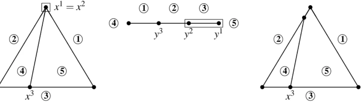
Kohlberg and Mertens (1986) define strategic stability of equilibria. Basically, a set of equilibria is called stable if every game nearby has equilibria nearby (Wilson, 1992). In degenerate games, certain equilibrium sets may not be stable. In the bimatrix game(A,B) in (2.30), for example, all convex combinations of (x1,y1) and (x2,y2) are equilibria, where x1=x2= (0,0,1)> and y1= (0,1)> and y2= (13,23)>. Another, isolated equilib-rium is(x3,y3). As shown in the right picture of Figure 3.1, the first of these equilibrium
sets is not stable since it disappears when the payoffs to player 2 for her second strategy 5 are slightly increased.
• • • •
°4
°1 °2 °3
°5
y3 y2 y1
·· ·· ·· ·· ·· T T T T T T T T T T ¥¥ ¥¥ ¥¥ ¥¥ ¥¥ • • • • °3 °1 °4 °5 °2
x3
x1=x2
·· ·· ·· ·· ·· T T T T T T T T T T • • • °3 °1 °5 °2 °4 • •¥¥ ¥¥ ¥¥ ¥¥ x3
Figure 3.1. Left and center: Mixed strategy sets X and Y for the game(A,B) in (2.30) with labels similar to Figure 2.2. The game has an infinite set of equilibria indicated by the pair of rectangular boxes. Right: Mixed strategy set X where strategy 5 gets slightly higher payoffs, and only the equilibrium (x3,y3) re-mains.
Wilson (1992) describes an algorithm that computes a set of simply stable equilibria. There the game is not perturbed arbitrarily but only in certain systematic ways that are easily captured computationally. Simple stability is therefore weaker than the stability concepts of Kohlberg and Mertens (1986) and Mertens (1989, 1991). Simply stable sets may not be stable, but no such game has yet been found (Wilson, 1992, p. 1065). However, the algorithm is more efficient and seems practically useful compared to the exhaustive method by Mertens (1989).
The perturbations considered for simple stability do not apply to single payoffs but to pure strategies, in two ways. A primal perturbation introduces a small minimum prob-ability for playing that strategy, even if it is not optimal. A dual perturbation introduces a small bonus for that strategy, that is, its payoff can be slightly smaller than the best payoff and yet the strategy is still considered optimal. In system (2.20), the variables x0,y0,r,s are perturbed by corresponding vectors ξ,η,ρ,σ that have small positive components,
ξ,ρ∈IRM andη,σ ∈IRN. That is, (2.20) is replaced by
A(y0+η) +IM(r+ρ) =1M
B>(x0+ξ) +IN(s+σ) =1N.
(3.1)
If (3.1) and the complementarity condition (2.24) hold, then a variable xi or yj that is zero
is replaced byξi or ηj, respectively. After the transformation (2.19), these terms denote
a small positive probability for playing the pure strategy i or j, respectively. Soξ andη represent primal perturbations.
Similarly, ρ andσ stand for dual perturbations. To see thatρi or σj indeed
ξ =0 for the example (2.30): ·
1 0 4
0 2 4
¸ x
0 1 x02 x03
+
µ
s4+σ4 s5+σ5
¶ =
µ
1 1
.
If, say, σ5>σ4, then one solution is x01=x20 =0 and x03= (1−σ5)/4 with s5=0 and s4=σ5−σ4>0, which means that only the second strategy of player 2 is optimal, so the higher perturbationσ5 represents a higher bonus for that strategy (as shown in the right picture in Figure 3.1). Dual perturbations are a generalization of primal perturbations, lettingρ=Aη andσ =B>ξ in (3.1). Here, only special cases of these perturbations will be used, so it is useful to consider them both.
Denote the vector of perturbations in (3.1) by
(ξ,η,ρ,σ)>=δ = (δ1, . . . ,δk)>, k=2(m+n). (3.2)
For simple stability, Wilson (1992, p. 1059) considers only special cases of δ. For each i∈ {1, . . . ,k}, the component δi+1 (or δ1 if i=k) represents the largest perturbation by some ε >0. The subsequent components δi+2, . . . ,δk,δ1, . . . ,δi are equal to smaller
perturbationsε2, . . . ,εk. That is,
di+j=εj if i+j≤k,
di+j−k=εj if i+j>k,
1≤ j≤k. (3.3)
Definition 3.1. (Wilson, 1992.) Let (A,B)be anm×nbimatrix game. Then a connected set of equilibria of(A,B)is calledsimply stableif for alli=1, . . . ,k, all sufficiently small ε>0, and (ξ,η,ρ,σ) as in (3.2), (3.3), there is a solution r= (x0,y0,r,s)> ≥0 to (3.1) and (2.24) so that the corresponding strategy pair(x,y)defined by (2.19) is near that set.
Due to the perturbation, (x,y) in Definition 3.1 is only an “approximate” equilib-rium. Whenε vanishes, then (x,y) becomes a member of the simply stable set. A per-turbation with vanishing ε is mimicked by a lexico-minimum ratio test as described in Section 2.6 that extends step (b) of Algorithm 2.9. The perturbation (3.3) is therefore easily captured computationally. With (3.2), (3.3), the perturbed system (3.1) is of the form (2.31) with
z= (x0,y0,r,s)>, C=
·
0 A IM 0
B> 0 0 IN ¸
, q=
· 1M 1N ¸
(3.4)
and Q= [−Ci+1, . . . ,−Ck,−C1, . . . ,−Ci]if C1, . . . ,Ck are the columns of C. That is, Q is
just−C except for a cyclical shift of the columns, so that the lexico-minimum ratio test is easily performed using the current tableau.
The algorithm by Wilson (1992) computes a path of equilibria where all perturba-tions of the form (3.3) occur somewhere. Starting from the artificial equilibrium (0,0),