ELECTROMAGNETIC SIDE-CHANNEL ANALYSIS ON INTEL ATOM PROCESSOR

(1)

ELECTROMAGNETIC SIDE-CHANNEL ANALYSIS

ON INTEL ATOM PROCESSOR

A Major Qualifying Project Report:

submitted to the Faculty

of the

WORCESTER POLYTECHNIC INSTITUTE

by

Anh Do

Soe Thet Ko

Aung Thu Htet

Date: April 15, 2013

Approved:

Professor Thomas Eisenbarth, Advisor

(2)

Abstract

Side-channel attacks, in particular, power analysis attacks, have gained significant attention in recent years because they can be conducted relatively easily, yet are powerful. Two types of attacks are investigated in this project: Simple Electromagnetic Analysis (SEMA), which is extremely eﬀective against asymmetric cryptography such as Rivest-Shamir-Adleman Algorithm (RSA) and Diﬀerential Electromagnetic Analysis (DEMA), which is commonly implemented against symmetric cryptography such as Advanced Encryption Standard (AES). This project implements SEMA and DEMA attacks based on the electromagnetic radiation from the Intel Atom Processor during its execution of cryptography algorithms.

(3)

List of Figures

1.1 Basic AES Algorithm . . . 9

1.2 Detail Structure of an AES encryption . . . 10

1.3 Internal Structure of an AES round . . . 11

1.4 Input 4⇥4 matrix . . . 11

1.5 Lookup Table used in Byte Substitution Layer . . . 12

1.6 Input and Output States of the ShiftRows sub-layer . . . 12

1.7 Matrix Operation in MixColumn sub-layer . . . 13

1.8 Key schedule for AES-128 . . . 14

1.9 Function g of Round i . . . 15

2.1 Project Setting Block Diagram . . . 18

2.2 General Project Setting . . . 18

2.3 Atom Board Setup . . . 19

2.4 Power Supply to the Amplifier . . . 20

2.5 Probe at the Serial COM Port . . . 23

2.6 Trigger Produced at the Serial Port . . . 24

2.7 Probe at the LPT Port . . . 25

2.8 Trigger Produced at LPT port . . . 26

2.9 Trigger Channel Setup . . . 27

(7)

2.11 RSA sampling setup . . . 28

2.12 AES Sampling Setup . . . 28

3.1 Original RSA Trace with 80 bit exponent (sim80_2.5G_2.trc) . . . 30

3.2 Spectrogram of the original trace (sim80_2.5G_2.trc) . . . 32

3.3 Trace after the 1st filter (sim80_2.5G_2.trc) . . . 33

3.4 Spectrum of the rectified trace (sim80_2.5G_2.trc) . . . 34

3.5 Trace after the 2nd filter (sim80_2.5G_2.trc) . . . 35

3.6 Automatically distinguish between MUL and SQ . . . 36

3.7 Simple RSA 1024 bit traces: Top - Raw trace. Middle - After the 1st _{filter. Bottom - After} the 2nd _{filter (sim1024_250M_2.trc) . . . .} ₃₈

3.8 Distinguish between MUL (red) and SQ (blue) . . . 39

3.9 Reconstructed key vs. Original key(sim256_250M_2.trc) . . . 40

3.10 80-bit key RSA filtered trace - GMP library . . . 42

3.14 80-bit key RSA filtered trace - OpenSSL library . . . 49

4.1 A sample AES trace . . . 55

4.2 Extracted AES region from the raw trace . . . 56

4.3 Frequency Spectrum Plot of Raw AES . . . 57

4.4 Filtered AES . . . 58

4.5 Extracted AES Operation . . . 59

4.6 Nine diﬀerent AES operations . . . 60

4.7 Downsampled AES written into Text Files . . . 60

(8)

4.9 All electromagnetic traces . . . 62 4.10 Correlation values for 256 possible keys . . . 63

(9)

List of Tables

1.1 Short Public Exponents for RSA . . . 6

1.2 Number of Rounds as a function of Key Length . . . 9

3.1 Window size and Pre-computations - GMP Library . . . 47

3.2 Window size and Pre-computations - OpenSSL Library . . . 52

(10)

Chapter 1

Introduction

1.1 Project Motivation

This section give a brief background of cryptography, side-channel attacks, and how they motivate us to conduct side-channel analysis on an Intel Atom Processor.

1.1.1 Cryptography

Encryption is the primary cryptographic technique to achieve confidentiality of messages between two com-municating parties over public networks. Nowadays, most of the cryptographic applications are conducted over digital media. To cite a few, applications include ATM cards, computer passwords, electronic commerce, etc. In such applications the encryption process typically involves two parties: encryption at the sender side and decryption at the receiver side. Encryption is the process of converting the original message (called plain-text) into a secret coded message (called ciphertext). Decryption achieves the reverse, i.e. reconstructing the plaintext from the received ciphertext. The encryption algorithm uses a key, i.e. a secret, which when combined with a mathematically defined algorithm renders the plaintext into an unintelligible ciphertext. At the receiving end, the key is used to decrypt the code and restore the original message. The greater the number of bits in the secret key, the more possible key combinations and the harder it would take to break the code using an exhaustive search strategy.

(11)

There are two major categories of encryption schemes: symmetric and asymmetric encryption schemes. In the symmetric key category, both the sender and receiver use the same key to encrypt and decrypt. A prominent example is the Advanced Encryption Standard (AES) algorithm which will be described later in Section §1.4. In symmetric ciphers encryption and decryption primitives are much faster than in public key algorithms. However securely delivering the secret key to the recipient in the first place might be a problem. In contrast, primitives in the second category use a key pair. Each recipient has a private key that is kept secret and a public key that is published for everyone. The sender uses the recipient’s public key to encrypt the message, and the recipient uses the private key to decrypt the message. The RSA public key scheme, described later in Section §1.2, is a good example of the schemes in this category.

1.1.2 Side-channel Attacks

There are several kinds of attacks on cryptographic devices. They share the same goal, to reveal the secret keys of the devices, but diﬀer significantly in terms of cost, time, equipment, and expertise needed. These methods could be categorized as follows:

• Invasive Attacks: The device is depackaged, and diﬀerent components of the device are accessed directly using a probing station. These attacks are extremely powerful but require quite expensive equipments and may be very diﬃcult to perform under some circumstances.

• Semi-invasive Attacks: The device is depackaged, but no direct electrical contact to the surface is made. These attacks are powerful, and do not require as expensive equipments as invasive ones. However, the process of locating the right position for an attack requires quite some time and expertise.

• Noninvasive Attacks: Only directly accessible interfaces of the device are exploited, and therefore no evidence of an attack is left behind. These attacks can be conducted with relatively inexpensive equipments, and hence, they pose a serious practical threat to the security of cryptographic devices. Most of the cryptographic schemes in use have been heavily investigated by cryptography experts to withstand powerful mathematical attacks. In contrast, most of the very same techniques have been shown to be vulnerable to attacks targeting their implementations through so-calledside-channel attacks[4]. Side-channel

(12)

attacks, in particular, electromagnetic analysis attacks based on the devices’ radiation, have gained quite attention in recent years because they are very powerful and can be conducted relatively easily. These attacks exploit the fact that the instantaneous electromagnetic radiation of a device depends on the data it processes and on the operation it performs [7]. There are two main types of power analysis attack: Simple Electromagnetic Analysis (SEMA), which is extremely effective against asymmetric cryptography and Differential Electromagnetic Analysis (DEMA), which is extremely effective against symmetric cryptography. The detail procedures of these two attacks will be discussed more in Section §1.5 and Section §1.3.

1.1.3 Motivation

Our project involves implementation of a side-channel attack on Intel Atom Processor. In 2008, Intel in-troduced the processors Silverthorne and Diamondville, which were both released under the name of Atom [1]. Intel targets the Silverthorne for mobile internet devices and Diamondville for personal computers. Intel Atom processors are high speed, and high performance embedded processors, and they are quite resistant to side-channel attacks. The fact that it is challenging to implement side-channel attack on Atom board is one of our project motivations. Another project motivation is the widespread use of Atom processors. They are used in everyday electronic devices, from net books to various embedded applications. The Pine Trail Architecture used in Atom Processors brings considerable power saving and improved performance [2]. Therefore, instead of heavy quad core processors, Atoms Processors are used in devices such as Net books, net-tops, and smartphones, which are used for simple applications such as browsing the internet. With such a wide field of application, Atom processor is a practical application in real-world that is worth investigating for side-channel analysis.

1.2 Rivest – Shamir – Adleman (RSA) Algorithm

The RSA algorithm is currently the most widely deployed public key cryptographic scheme. In practice, RSA is mostly used for encryption of small pieces of data such as key transport, digital signatures and digital certificates on the Internet. Since it is several times slower than symmetric ciphers due to its computational complexity, RSA is often used together with a symmetric cipher such as AES, where AES does the actual

(13)

bulk data encryption. With the use of both public key and private key, RSA has an important role to securely exchange a key for a symmetric cipher. Moreover, the underlying reason for the RSA algorithm is based on the integer factorization problem: Multiplying two large primes is computationally easy, while factoring the resulting product is very hard. In this section, again all the explanation of the AES algorithm is advised from the book “Understanding cryptography a textbook for students and practitioners” [10].

1.2.1 Encryption and Decryption

Both RSA encryption and decryption are performed in the integer ring Zn with modular arithmetic as the main computation.

Encryption: Given the plaintext x, and the public keykpub= (n, e), the encryption function is

y=ekpub(x)⌘x

e _mod_n

Decryption: Given the ciphertext y, and the private keykpr= (d), the decryption function is

x=dkpr(y)⌘y

d _mod_n

where x, y₂Zn

In practice, x, y, n, and d are very large integers, i.e. usually 1024 bits long or more. The value e is called the public exponent or encryption exponent, while the private key d is called the private exponent or decryption exponent. Based on the algorithm, here are some essential requirements for the RSA crypto-system:

• It must be computationally infeasible to determine the private key d given the public key e and n

• The maximum bit length that could be encrypted is the size of the modulus n

• A method for fast exponentiation with long numbers is need

(14)

1.2.2 Detail Implementation of RSA

1.2.2.1 Key Generation

During the setup phase, the RSA public key and private key are computed as follows.

• Choose two large primes p and q

• Compute the modulusn=pq

• Compute (n) = (p 1)(q 1)

• Select the public exponente2{1,2. . . (n) 1}such that gcd(e, (n)) = 1

• Compute the private key d such thatd⌘e 1 _{mod (n)}

1.2.2.2 Fast Exponentiation

As stated above, RSA requires a fast exponentiation method for both encryption and decryption processes. The square-and-multiply algorithm is the most simple and commonly used for this purpose.

• Scanning the bits of the exponent H from the left (MSB) to the right (LSB)

• In every iteration, square (SQ) the current result

• If and only if the current bit is 1, multiply (MUL) the current result by the base x In general, for an exponent H with a bit length of t+1, the numbers of operations needed are

#SQ=t, #M U L= 0.5t, #T otal= 1.5t

1.2.2.3 Fast Encryption with Short Public Exponents

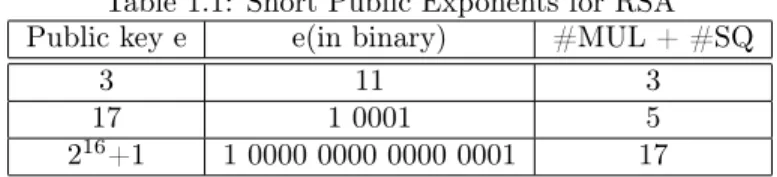
A surprisingly simple yet powerful trick can be used to accelerate the encryption of a message and verification of an RSA signature is choosing the public key e. For this purpose, the public key is chosen to be a small value with low Hamming weight. Here are the three most common values are shown in Table 1.1.

(15)

Table 1.1: Short Public Exponents for RSA Public key e e(in binary) #MUL + #SQ

3 11 3

17 1 0001 5

216₊₁ _{1 0000 0000 0000 0001} ₁₇

1.2.2.4 Fast Decryption with the Chinese Remainder Theorem

Unlike the public exponent, the private key d cannot be short since an attacker could simply brute-force all the possible numbers up to a given bit length. In practice, e is often chosen to be short, while d has full bit length. Thus, the Chinese Remainder Theorem (CRT) is applied to accelerate RSA decryption and signature generation. The 2 large primes, p and q, in the key generation phase are used in this transformation.

• In the first step, transformation into the CRT domain proceeds as follows.

yp⌘y modp, yq⌘y modq, dp ⌘d mod (p 1), dq ⌘d mod (q 1) • In the second step, we compute the exponentiation in the CRT domain as follows.

xp⌘ypdp modp, xq ⌘yqdq modq

• Finally, the inverse transformation is computed asx_⌘qcpxp+pcqxq modnwhere the coeﬃcients are

computed ascp⌘q 1 modp, cq ⌘p 1 modq

1.2.2.5 Finding Large Primes

During the key generation process, an important aspect is to find two large primes p and q. The general approach is to generate integers at random then check for primality. This process depends on two important questions, “How common are primes?” and “How fast is the primality check?”. It turns out that even for large value, the density of primes is still suﬃciently high. In fact, the probability for a random odd number to be prime:

P(p is prime) = 2 lnp

(16)

Moreover, the primality tests are also computationally inexpensive. Examples are the Fermat test, the Miller – Rabin test, and variants of them.

1.2.3 RSA in Practice

The RSA system described so far has several weaknesses.

• RSA encryption is deterministic, one-to-one mapping for a specific key

• Plaintexts x = 0, -1 , 1 produce ciphertexts equal to 0, 1, -1

• Small public exponents and small plaintexts might be subject to attack

• Ciphertexts are malleable. A crypto scheme is said to be malleable if the attacker is capable of trans-forming the ciphertext into another ciphertext which leads to a known transformation of the plaintext. In the case of RSA, if the attacker computes a new cipher text se_{y with s is some integer, then the} receiver decrypts the manipulated ciphertext as(se_y)d _⌘_sed_xed _⌘_sx _mod_{n. These manipulations}

might do harm since the attacker is able to get s times the plaintext.

A possible solution to all these problems is the use of padding, which embeds a random structure into the plaintext before encryption. A modern technique, Optimal Asymmetric Encryption Padding (OAEP), for padding RSA messages is specified and standardized in Public Key Cryptography Standard #1 (PKCS #1) [12]. On the decryption side, the structure of the decrypted message has to be verified.

1.3 Simple Electromagnetic Analysis (SEMA) Attacks on RSA

Here are the few common attacks on the RSA.

• Protocol attacks: exploit weaknesses in the way RSA is being implemented. Many of them can be avoided by using standard padding.

• Mathematical attacks: the best method is factoring the modulus. These attacks can be prevented by choosing a suﬃciently large modulus.

(17)

• Side-channel attacks: exploit information about the private key which is leaked through physical chan-nels such as power consumption and timing behavior. This now becomes a large and active filed of research in modern cryptography.

For this project, we apply a side-channel attack called the simple electromagnetic analysis method. The attacker will be able to find out the private key by observing the decryption process revealed by the devices’ radiation, which is the exponential algorithm that has been demonstrated before. Therefore the attacker can decipher the encrypted text with both the public key and the private key. The exponential algorithm has been applied in many RSA cryptographic implementations. As the exponential algorithm has been illustrated in the previous session, there are only 2 diﬀerent operations, square and multiply. The sequence of these limited operations composing the private key can be revealed by visual observation of the electromagnetic traces.

1.4 Advanced Encryption Standard (AES) Algorithm

The Advanced Encryption Standard Algorithm is the most widely used symmetric cipher today. The AES block cipher is also mandatory in several industry standards and is used in many commercial systems. In this section, all the explanation of the AES algorithm is advised from the book “Understanding cryptography a textbook for students and practitioners” [10]. In addition, all the figures are redrawn from the ones in this book.

1.4.1 Overview Structure

A general AES round is shown in Figure 1.1. The input x is a 128-bit block of data or plaintext. The key, denoted by k, can be 128 bits, or 192 bits, or 256 bits. The output y is the 128-bit ciphertext.

(18)

Figure 1.1: Basic AES Algorithm

An AES algorithm consists of several transformation rounds or cycles which convert the input plaintext to the output ciphertext. For diﬀerent key lengths, the number of rounds varies as shown in Table 1.2. For example, if the key length is 128 bit, there will be 10 AES rounds.

Table 1.2: Number of Rounds as a function of Key Length Key Length Number of rounds

128 bits 10

192 bits 12

256 bits 14

The complete AES block diagram is shown below in Figure 1.2. The initial round, or round 0, consists of only one Key Additional Layer. Next, the sequence of AES rounds is consecutively performed, taking the output of the previous round as the current input. Each AES round consists of three so-called layers that manipulate the input data, which are

• Byte Substitution Layer: The data is transformed nonlinearly by using a lookup table, called the S-box, which has special mathematical properties. This nonlinear transformation causes confusion and randomization to the data; in other words, changes in individual state bits spread quickly across data path.

• Diﬀusion Layer: This layer provides diﬀusion over all state bits. It has two sublayers: ShiftRows Layer, and MixColumn Layer, both of which are linear transformations. The former performs byte-wise permutation to the data, and the latter performs matrix operation in order to mix or combine bytes of data.

(19)

• Key Addition Layer: the 128-bit round key or sub-key is combined with the current state by XOR operation. The sub-key is derived from Key Schedule which will be mentioned in details later in 1.4.4. The output of the last round is also the final output of the AES cipher. However, the last round does not include MixColumn sublayer in the Diﬀusion Layer.

Figure 1.2: Detail Structure of an AES encryption

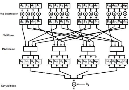
1.4.2 Internal Structure of AES

The internal implementation of a single round of AES is shown in Figure 1.3. First, the 128-bit plaintext is separated into 16 bytes, from A0 to A15. Each byte is then fed into the S-Box (Byte Substitution Layer). The 16-byte output from the S-box, from B0 to B15, is permuted byte-wise in the ShiftRows Layer. The result is mixed and combined in the MixColumn Layer, resulting in the intermediate value, from C0 to C15.

(20)

The intermediate value is then XORed with the 128-bit round key in the Key Addition Layer before going to the next round.

Figure 1.3: Internal Structure of an AES round

1.4.3 Detail Implementation of each Layer

For convenience, the bytes of 16-byte input data is arranged in a 4⇥4 matrix, as shown in Figure 1.4.

Figure 1.4: Input 4⇥4 matrix

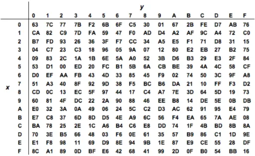
In Byte Substitution Layer, the bytes are transformed nonlinearly using the S-box, shown in Figure 1.5. For example, if the input byte is E9 in hexadecimal, the output is the element in row number E and column number 9, which is 1E in hexadecimal.

(21)

Figure 1.5: Lookup Table used in Byte Substitution Layer

The detail implementation of the ShiftRows sublayer is shown in Figure 1.6. The input state, a 4⇥4 matrix from B0to B15, is the output from the Byte Substitution Layer. To achieve the output state, the first row of the matrix is unchanged, the second row is shifted one position to the left, the third row is shifted two positions to the left, and the fourth row is shifted three positions to the left.

Figure 1.6: Input and Output States of the ShiftRows sub-layer

The new 4⇥4 matrix is fed into the MixColumn sublayer, and the output is calculated using the special matrix operation employing Galois Field Properties, as shown in Figure 1.7. Each column of the output matrix is calculated by performing the matrix operation with the corresponding column of the input 4⇥4

(22)

matrix.

Figure 1.7: Matrix Operation in MixColumn sub-layer

Finally, the Key Addition Layer takes in two inputs: the current 16-byte state matrix, which is output from the MixColumn sublayer, and a round key. The output is obtained by performing XOR addition of these two inputs.

1.4.4 Key Schedule

There are diﬀerent key schedules for three AES key sizes of 126, 192, and 256 bits. As all of the schedules are fairly similar, only the schedule for 128-bit key length will be discussed in detail. For the 128-bit key, there are 10 rounds in the AES encryption operation. However, there is an XOR addition of key before the first round. This means we need 11 sub-keys or round keys.

The key expansion process of an AES-128 is demonstrated in Figure 1.8. The input is the 128-bit original key, represented as bytes from K0through K15.Note that the key schedule is word-oriented, and the 11 sub-keys are stored in a key expansion array as words from W[0] through W[43]. The first sub-key is obtained by directly copying the original key from the four elements W[0], W[1], W[2], and W[3] of the array. The remaining 10 sub-keys are computed recursively, using an XOR addition and a non-linear function g, which will be discussed later.

(23)

Figure 1.8: Key schedule for AES-128

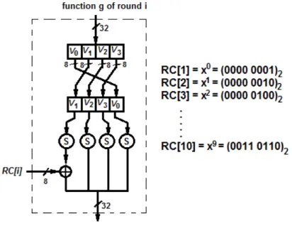
As stated, function g plays an important role in sub-key derivation as it adds non-linearity to the key schedule. It takes four input bytes and produces four-byte output, as shown in Figure 1.9. It first rotates the input bytes, and then performs a byte-wise S-Box substitution. A round coeﬃcient (RC) is added to the leftmost S-Box output byte. The RC value is an element of Galois field and varies from round to round.

(24)

Figure 1.9: Function g of Round i

1.5 Di

ﬀ

erential Electromagnetic Analysis (DEMA) Attacks on AES

The Differential Electromagnetic Analysis attack exploits the dependence of power consumption on interme-diate values, which is very similar to the Differential Power Analysis attack [5]. Compared to the SEMA attack, the DEMA attack has two main advantages. First, a DEMA attack doesn’t require detailed knowl-edge about the cryptographic device. It is usually sufficient to know the cryptographic algorithm executed by the device. Second, a DEMA attack works even if the recorded electromagnetic traces are extremely noisy. Mainly, the DEMA attack analyzes the dependence of electromagnetic radiation on the processed data at fixed moments of time. The general strategy for a DEMA attack consists of five steps.

• An intermediate result of the executed algorithm is chosen for the attack. It has to be a function of d (plaintext or ciphertext) and k (a small part of the key).

• D diﬀerent data blocks are fed to the device for encryption or decryption, and the corresponding electromagnetic traces are recorded. The input data blocks are denoted as a vectord={d1, d2. . . dD}.

(25)

matrix T of dimension D by T is constructed by using the recorded electromagnetic traces.

• Hypothetical intermediate values are calculated for every possible key. The key hypotheses are repre-sented as a vectork=_{k1, k2. . . kK}. Then, the data vector d and key vector k are used to compute

intermediate values to get matrixV = [vij], where vij =f(di, kj).

• The intermediate values in matrix V are mapped to the electromagnetic radiation values, resulting in a new matrix H of hypothetical electromagnetic radiation values. Most common methods for doing so are Hamming Weight Model, Hamming Distance Model and Zero Value Model.

• Hypothetical electromagnetic radiation values in matrix H are compared with the actual electromagnetic traces. The correlation coefficient between each column hi of matrix H and each column tj of matrix T are calculated and stored in a new K⇥T correlation coefficient matrix R. The correct key can be retrieved by looking at the index of the largest correlation coefficient value in the matrix R. The row number indicates the correct key and the column number indicates the time.

(26)

Chapter 2

Project Setting

This section discusses the experimental settings of our project, including installing the cryptography libraries, compiling the C codes, and capturing electromagnetic traces.

2.1 Overview

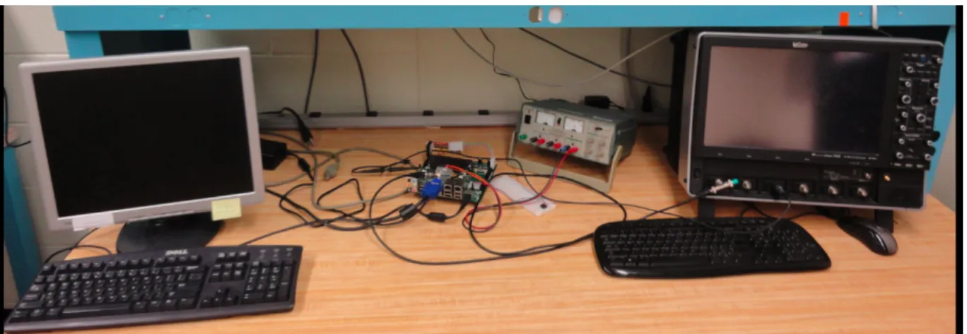
The block diagram of the project setting is shown in Figure 2.1. In the center, the Intel Atom Board is operated on UBUNTU 12.04.1 OS, connected to a keyboard and a monitor. These standard I/O devices assist the process of writing and compiling the code. The board itself also has two USB ports, used for copying the library installation files as well as the code from other computers. From the board, either the serial port or the LPT port is connected to a channel of the oscilloscope in order to send the trigger, which will be discussed later in Section §2.3. During the cryptography execution, the electromagnetic waves are collected by a 3-loop coil antenna, with a diameter of about 1 centimeter. The antenna plus an amplifier, which is powered 15V by power supply, can detect electromagnetic leakage traces from Intel Atom Board, and send them directly to a channel of the oscilloscope. The scope model is WavePro 725Zi from LeCroy with the bandwidth of 2.5GHz and the maximum sampling rate of 40 GS/sec [6]. Based on the trigger sent from another channel, the oscilloscope is able to capture the traces from a chosen channel at the right moment, then write to binary files, and save them to the hard disk. The trace files are then transferred to other

(27)

computers via a USB drive in order to perform signal analysis in MATLAB.

Figure 2.1: Project Setting Block Diagram

Based on the block diagram, the actual project setting is shown in Figure 2.2. The Intel Atom Board is in the middle, run on Linux system. To the left is the monitor and the keyboard, which are the standard I/O connected to the board. The antenna coil with the amplifier is placed above the board in order to capture the electromagnetic waves, and the probe is connected to the serial port, or LPT port of the board. These placements can be seen more clearly in the close-up pictures, Figure 2.3, Figure 2.4, and Figure 2.7. Based on the trigger from a channel, this oscilloscope will collect the electromagnetic traces of the Atom board from another channel and save them to the hard disk. In the back is the power rail supplying for all devices, including the monitor, the Atom board, the oscilloscope, and the power supply.

Figure 2.2: General Project Setting

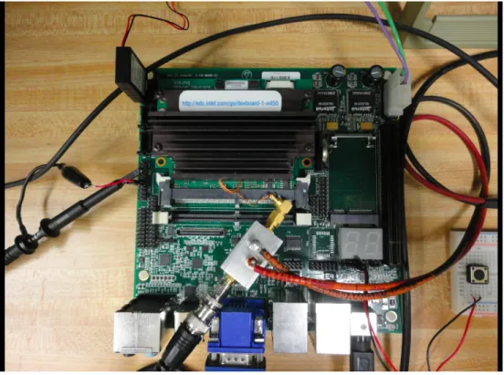
A close-up view on the Intel Atom Board is shown in Figure 2.3. The board uses EMPhase S1 series flash module for memory. To the left, the oscilloscope probe is connected to the serial port in order to detect the

(28)

generated trigger. In the middle, the coil antenna is placed above the board and under the heat-sink to capture the electromagnetic waves. The optimum position is chosen based on trial-and-error in order to maximize the trace amplitudes while minimize the unexpected noise from other parts. Interestingly, the optimum positions for the RSA and AES traces are different, which makes sense since these two algorithms require different operations of the system. For these two algorithms, the coil antenna measures the electromagnetic radiations from different capacitors in the board.

Figure 2.3: Atom Board Setup

The amplifier of the antenna coil is connected to the power supply as shown in Figure 2.4. The amplifier with the model number Mini-circuit ZFL-1000LN+, amplifies the signal inside the range 0.1 MHz to 1000 MHz, before it goes to the oscilloscope. This filter range is suﬃcient since the RSA and AES operations, as later described, are in the order of 10 MHz to 100 MHz. The amplifier has a minimum gain of 20dB [8]. To the right, the Atom board is connected to a simple button on a breadboard. This button is used to start up or reset the whole system when necessary.

(29)

Figure 2.4: Power Supply to the Amplifier

2.2 Writing the C Code

This section explains how we installed cryptography libraries on Linux System, and how we compiled C codes to implement RSA and AES algorithms.

2.2.1 Employing the Libraries

In order to quickly perform the RSA and AES algorithms, it is convenient to employ free public libraries inside the C code. For this project, two popular libraries are chosen: the GNU Multiple Precision Arithmetic (GMP) library version 5.1.0 [13], and the OpenSSL library version 1.0.1c [9]. The GMP library is well-known for the speed when dealing with long integers (bignum) using highly optimized assembly language; thus, it will be used to implement the RSA algorithm, both simple multiply-and-square method and modular exponentiation method. The OpenSSL library is an open-source implementation of the SSL and TLS protocol,

(30)

which implements many basic cryptography functions. Hence, the library consists of both RSA and AES implementations.

These two library packages can be downloaded from their main websites. The installation process is also simple. Here is an example of installing the OpenSSL library. The first step is to extract files from the downloaded package. The second step is to enter the directory where the package is extracted, and to run the configuration file with the default setup. Next step is to compile OpenSSL and to check for any error messages. The last step is to install the OpenSSL library with root command for privileges on destination directory.

tar -xvzf OpenSSL-1.0.1c.tar.gz ./config

make

sudo make install

Now, the library is ready to be used by including the library header in the beginning of the C code, for example:

#include <OpenSSL/aes.h>

2.2.2 Compiling the Code

Since the compiler of the system doesn’t link the library automatically, we have to specify the library directory manually in each compilation. To compile the code using the GMP library, use the command:

gcc -I/usr/local/include test.c /usr/local/lib/libgmp.a

To compile the C code using the OpenSSL library, use the command:

(31)

2.3 Generating Triggers

Generating the trigger is a very important factor in the process of capturing the electromagnetic traces since the oscilloscope need to be triggered based on one of its channel inputs. For both RSA and AES implementations, the atom board first generates the trigger at one of its output port. Since there is always a rising time at the output port when going from low to high, the board is forced to sleep or to perform some delay to accommodate this latency. Then, the cryptographic algorithm is performed, followed by another delay period, either sleeping or counting. The procedure ensures that the whole cryptographic algorithm is captured in the electromagnetic trace, and reduces the interference between two consecutive operations.

2.3.1 From the Serial Port

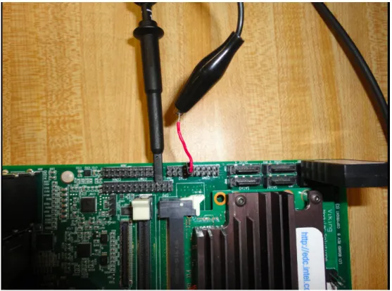
Since the serial port is quite common in many systems and easy to be written to, we use it as the trigger when capturing the RSA electromagnetic traces. The oscilloscope probe is connected to the serial port as shown in Figure 2.5. The ground is connected to the pin 6 while the probe is connected to the pin 3 of the serial COM port.

(32)

Figure 2.5: Probe at the Serial COM Port

At the beginning of the code, we perform test I/O for this specific port using the command:

fd = open("/dev/ttyS0", O_RDWR|O_NOCTTY|O_NDELAY);

Next, every time a trigger is needed, we just have to write a single bit 1 to that port:

write(fd,tpstr,1);

After a finite time, the output port is back to 0; thus, we don’t have to manually turn oﬀ the port before the next trigger. The trigger produced at this serial port is shown in Figure 2.6. Since the oscilloscope is set with 1µs per division, the trigger rising time is about 0.75µs, which is significantly slow. However, since the RSA algorithm itself is slow as well, in an order of 10 milliseconds, it is still acceptable to use this trigger when collecting the RSA traces.

(33)

Figure 2.6: Trigger Produced at the Serial Port

2.3.2 From the LPT Port

Since a single AES takes about 1.2µs, the trigger from the serial port, which has a latency of about 0.75µs, is not sufficient. Instead, we need a very fast trigger to capture the AES on the oscilloscope. We researched about Intel Atom Board [3] in order to find a port that can produce a trigger with fast rising time. Finally, we came up with the conclusion of using the LPT (Parallel) port. Although LVDS (low voltage differential signal) port and LPC (low pin count) seem promising as they potentially have lower latencies, producing a trigger at those ports may be difficult due to involving low-level programming such as changing the kernel, and bios setting.

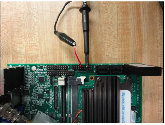
The oscilloscope probe is connected to the data pin of the LPT port as shown in Figure 2.7. The ground is still connected to the pin 6 of the serial COM port while the probe is connected to any pin of the LPT port.

(34)

Figure 2.7: Probe at the LPT Port

To write to the data bits of the LPT port, a general procedure is implemented in C. First, the base port address is defined as below:

#define BASEPORT 0x378 /*lp1*/

Next, we have to set the permission to access the port:

if (ioperm(BASEPORT, 3, 1)) {perror("ioperm"); exit(1);}

Inside the main function, whenever a trigger is needed, we just have to write a sequence of 1 to the chosen port:

outb(255, BASEPORT);

(35)

outb(0, BASEPORT);

Finally, for our own safety, we have to take away the permission to access the LPT port at the end of main function in case other codes use the port for diﬀerent purposes.

if (ioperm(BASEPORT, 3, 0)) {perror("ioperm"); exit(1);}

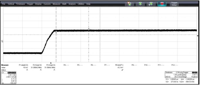
The trigger produced at this LPT port is shown in Figure 2.8. The oscilloscope is still set with 1µs per division, and as seen, the slope now is much steeper. The latency is only about 0.05µs, which is acceptable to use as the trigger when collecting the AES traces.

Figure 2.8: Trigger Produced at LPT port

2.4 Capturing the Traces

In order to successfully capture the interested electromagnetic trace, the scope setup has to be strictly followed. First step is to set up the trigger signal, which can be in any channel. In this case, we chose channel 3, with a positive edge trigger. Detail options are shown in Figure 2.9.

(36)

Figure 2.9: Trigger Channel Setup

Next step is to set up the trace signal, which in this case is chosen to be channel 1. The channel is coupling with AC1MW, and the bandwidth is set to 200 MHz, which is enough to cover the RSA and AES operations.

Figure 2.10: Trace Channel Setup

The final step is to set up the appropriate sampling rate in order to capture the whole operation in a single trace. For example, for the RSA 1024-bit key, the sampling rate needs to be 200MS/sec, as shown in Figure 2.11. For shorter or longer key length, the sampling rate would be modified accordingly.

(37)

Figure 2.11: RSA sampling setup

Sine the AES operations are really fast, the sampling rate can be set to the maximum of 20GS/sec, as shown in Figure 2.12.

(38)

Chapter 3

Attacking the RSA

3.1 General Procedure of Analyzing RSA Electromagnetic Traces

This section explains the standard procedure of collecting, filtering, and processing traces to clear unwanted noises and other operations of the system.

3.1.1 Collecting the Traces

As stated, we first set a trigger at the serial port, perform a sleep command, run one RSA operation, and then another sleep command. As the Atom Board executes this procedure over and over again in a loop, the oscilloscope records the traces based on the intended trigger. For each trace, general information of the key, the crypto algorithm, the library, and the scope setting are also recorded. An example trace is shown in Figure 3.1.

(39)

Figure 3.1: Original RSA Trace with 80 bit exponent (sim80_2.5G_2.trc)

• Trace name: sim80_2.5G_2.trc

• RSA Key: 80 bits (FFFF0000FFFF0000FFFF)

• RSA algorithm: Simple multiply-and-square, GMP library

• Sampling frequency: 2.5 GS/sec

Despite the noises, we can see the RSA operation in the middle of the trace, represented by the region with higher amplitude. The two regions with lower amplitude are when the board is performing the sleep commands. However, we cannot see any pattern of multiply and square operations in this raw trace; thus, filtering techniques are required in order to clear out unexpected factors from this trace.

3.1.2 Filtering Technique

Our SEMA attack on RSA utilizes two filters, and now we will describe the concept behind these filters in details. Since there are a lot of noises as well as other system operations running during the cryptography

(40)

execution, an appropriate band-pass is employed to amplify only the signal inside the range of the interested operations, i.e. RSA or AES. This would be the first filter applied to the collected traces.

The electromagnetic radiation of the target device could be given asp(t) =Pconst+pdyn(t)where Pconst

is the constant part and pdyn(t) is the dynamic part caused by internal operations. Usually, the dynamic portion is much weaker than the constant part. Thus, the possibility of exploiting leakage heavily depends on the quality of the isolation of pdyn(t).

Since the amplitude of the signal is modulated ass(t) = p(t) cos(!rt)where wris the carrier frequency, the extraction of p(t) or the weak dynamic portion pdyn(t) could be done using amplitude demodulation. In this project, a very common incoherent technique is employed, which based on rectification, or often called envelope detection. Here is a quick explanation of the method. Let first denote the frequency domain representation of the original signal asA(j!) =F{p(t)_}. Now the spectrum of the rectified signal could be computed [11].

F_{|s(t)_|}=F_{p(t)_|cos (!rt)|}=F

( p(t)2

⇡

1

X

⌫= 1

( 1)⌫

1 4⌫2e

j2⌫!rt )

F{|s(t)|}= 2

⇡

1

X

⌫= 1

( 1)⌫

1 4⌫2F p(t)e

j2⌫!rt ₌ 2

⇡

1

X

⌫= 1

( 1)⌫

1 4⌫2A(j! j2⌫!r)

Thus, the rectified signal is essentially similar to the spectrum of p(t), which however is scaled and repeated at all even multiples of the carrier frequency. Finally, an appropriate band-pass filter at low frequency is employed to isolate the desire signal p(t).

3.1.3 Filtering the Traces in MATLAB

The first step is to plot the spectrogram of the electromagnetic trace, as shown in Figure 3.2, in order to find which frequency range the RSA operations execute at. Thespectrogramfunction is available in the MATLAB Signal Processing Toolbox, and the detail script of plotting the spectrogram can be found in the Appendix. Since we add two sleep commands at the beginning and at the end, the RSA operation is expected to stand out clearly.

(41)

Figure 3.2: Spectrogram of the original trace (sim80_2.5G_2.trc)

As seen, the x-axis is the time in second, the y-axis is the frequency in Hz, and the color at each point represents the amplitude of the specific frequency at the specific time. Based on the spectrogram, we can observe several basic operations of the system, which can be seen as continuous red stripes from the beginning until the end. In other hand, since our RSA operation is set between two sleep commands, it would stand out as a single red stripe but be truncated at the two ends. Applying this concept to the current spectrogram, the RSA operation is the red stripe ranging from 50 MHz to 80 MHz. Moreover, noise can be seen as red spots appearing randomly in the spectrogram. Therefore, the first bandpass filter is chosen to be from 50 MHz to 80 MHz. This filter will attenuate the undesired noise as well as other operations performed by the Atom board during the experiment. The trace after the first filter is shown in Figure 3.3.

(42)

Figure 3.3: Trace after the 1st filter (sim80_2.5G_2.trc)

As expected, the first filter successfully reduces the noise and other operations of the system. The trace amplitude during RSA operation is much higher than the amplitude during sleep time. Also, the overall amplitude is more uniform. However, as mentioned in 3.1.2, the weak dynamic portion pdyn(t) has to be extracted using amplitude demodulation in order to exploit the information leakage. Therefore, the next step is the envelope detection based on rectification, which removes the carrier frequency from the current trace. After that, the multiply and square operations can be seen and diﬀerentiated much more easily. Unfortunately, since the carrier frequency is unknown, we first have to take the absolute value of the trace, which shifts the spectrum center to DC, and then plot the new spectrum in order to obtain some insights about the carrier frequency. The new spectrum is shown in Figure 3.4.

(43)

Figure 3.4: Spectrum of the rectified trace (sim80_2.5G_2.trc)

The spectrum of the rectified trace consists of a huge spike at DC and several smaller spikes around; one of them would be the carrier frequency we are looking for. By trial-and-error, we find out the closest spikes to DC, near 40 kHz, is the interested one. Thus, a second bandpass filter is set from 20 kHz to 40 kHz in order to remove the carrier frequency, and the new trace is shown in Figure 3.5.

(44)

Figure 3.5: Trace after the 2nd filter (sim80_2.5G_2.trc)

3.1.4 Finding the Key

After the envelope detection process, each operation can be visually identified clearly. In this case, the upper peaks are diﬀerent for the multiply and square operations, and will become the distinguisher. A longer peak represents a multiply operation while a shorter one represents a square operation. It is convenient to do the diﬀerentiation procedure automatically in MATLAB. First, we have to cut out the RSA part, perform the peak detection, and then use clustering method to separate between multiply and square operations. For visualization purpose, we draw letter M in red representing a multiply, and letter S in green representing a square near each peak. The processed trace with M and S displayed is shown in Figure 3.6.

(45)

Figure 3.6: Automatically distinguish between MUL and SQ

Finally, the sequence multiply and square can be converted to the RSA key of interest. Since this trace employs the multiply-and-square method, a square followed by of multiply corresponds to a single bit 1, while a single square corresponds to a single bit 0. Again, a MATLAB script is deployed to automatically convert the multiply-and-square sequence to a binary key. The script returns the keyFFFF0000FFFF0000FFFF in hexadecimal. Knowing the original key, we can then evaluate the performance of our method based on the bit error rate, which is computed by XOR-ing the received key with the original one. In this case, the bit error rate is zero; we successfully retrieve the secret key from the collected electromagnetic trace.

3.2 Simple Multiply-and-Square RSA

In this part, we employ the C code that implements a simple multiply-and-square RSA algorithm using the GMP library. Basically, the board scans the bits of the exponent from the left (MSB) to the right (LSB). In every iteration, it squares the current result. If and only if the current bit is 1, it multiplies the current

(46)

result by the base. The complete C code can be found under the Appendix. Below is a code snippet of the simple multiply-and-square RSA.

for( i = b i t s 1; i >= 0 ; i ) { mpz_mul(d , d , d ) ; % SQUARE mpz_mod(d , d , c ) ;

i f( mpz_tstbit (b , i ) == 1) {

mpz_mul(d , d , a ) ; % MULTIPLY mpz_mod(d , d , c ) ;

} }

In this part, we use a 1024 bit key, a standard key length for RSA. Using the trigger from the serial port, we can collect the electromagnetic traces and then start the analysis. Below is the general information of the trace, and the trace itself is shown in the top part of Figure 3.7.

• Trace name: sim1024_250M_2.trc

• RSA Key: 1024 bits {FA0BFC0DFE09F807F60543210(x10)F(x6)}

• RSA algorithm: Simple multiply-and-square, GMP library

• Sampling frequency: 250 MS/sec

Following the general filtering procedure, we first plot the spectrogram of the received electromagnetic trace to determine the frequency range of RSA algorithm. As usual, the RSA operation stands out clearly compared to the sleep time, ranging from 50 MHz to 80 MHz. Thus, we use these parameters as the first bandpass filter for the received trace. The result trace is shown in the middle part of Figure 3.7.

As seen, the trace is now much clearer and more uniform; the amplitude during RSA operation is much higher than the amplitude during sleep time. Next step is envelope detection, which removes the carrier frequency from the electromagnetic trace. We have to rectify the trace and then plot the spectrum to find the frequency of interest. Similarly, the spikes near 40 kHz is the one we are looking for. Thus, the second bandpass filter is chosen from 20 kHz to 40 kHz, the result trace after this filter is shown in the bottom part of Figure 3.7.

(47)

Figure 3.7: Simple RSA 1024 bit traces: Top - Raw trace. Middle - After the 1st _{filter. Bottom - After the} 2nd _{filter (sim1024_250M_2.trc)}

(48)

The multiply and square operations are now much clearer. In this case, the lower peaks are diﬀerent for the multiply and square operations, and will become the distinguisher. A deeper peak represents a multiply operation while a shorter one represents a square operation. It is convenient to do the diﬀerentiation procedure automatically in MATLAB. First, we have to cut out the RSA part, perform the peak detection, and then use clustering method to separate between multiply and square operation. The detail MATLAB script can be found in the Appendix. The peak heights are shown in the scatter plot, Figure 3.8. With clustering method, the script automatically separates the multiply operations in red and the square operations in blue.

Figure 3.8: Distinguish between MUL (red) and SQ (blue)

Next, the sequence of multiply and square operations can be converted to the RSA key of interest. Since this trace employs the multiply-and-square method, a square followed by of multiply corresponds to a single bit 1, while a single square corresponds to a single bit 0. Again, a MATLAB script is deployed to automatically convert the multiply-and-square sequence to a binary key. Then, the reconstructed key is plotted with red

(49)

stars together with the original key, which is plotted in blue lines, as shown in Figure 3.9.

Figure 3.9: Reconstructed key vs. Original key(sim256_250M_2.trc)

As seen, the reconstructed key matches with the original one really well. However, we have to make several small oﬀset adjustments due to the sliding between 0 and 1 since bit 0 corresponds to a single operation while bit 1 corresponds to two consecutive operations. The bit error rate is pretty small, only about 4%, which mostly came from the noise and the unexpected behaviors of the board. Performing the attack several times and calculating the key based on the majority rule can help us to improve the bit error rate.

3.3 Modular Exponentiation (RSA) - GMP Library

In this part, we perform an attack on the RSA algorithm of the GMP library, in particular, the modular exponentiation function. Instead of the simple multiply-and-square method, this library employs the sliding

(50)

window algorithm. Generally, sliding window exponentiation computes the power by looking at a number of exponent bits at a time, called the window size. Diﬀerent from the simple method, the sliding window method requires pre-computation of several values.

First step is to computex2 _{from the plain text x. Next, the system consecutively computes} _x3_, _x5_{, up} until x2k 1 _{where k is the window size. These values will be used for the multiplications in the next part.} Similar to the simple multiply-and-square method, the exponent bits are scanned from left to right. If the bit is 0, the current value is squared. Otherwise, if the bit is 1, the system finds the longest bit-string whose length is less than or equal to the window size, and the ending-bit is also 1. This bit-string will equal to one of the pre-computed values from the previous part; and the current value is multiplied directly with this bit-string. After scanning all the exponent bits, the final exponentiation is returned.

Despite the extra time at the beginning due to the pre-computations, the sliding window exponentiation is much faster the simple one. Multiplying with a stored bit-string instead of a base only saves a lot of computation time. The goal of our attack is still to distinguish between multiply and square operations; however, we might have to make an additional eﬀort to separate between multiplying of diﬀerent bit-string values. Otherwise, there would be several unknown bits inside the reconstructed key. For each multiplication, only the first bit and the last bit in the window is ensured to equal 1, while the middle bits could either be 0 or 1.

3.3.1 Di

ﬀ

erent Key Sizes

As expected, the GMP library employs diﬀerent window sizes for diﬀerent RSA key lengths. In this section, we explore the window size as well as the number of pre-computations as a function of the key length. For the convenience, the key is chosen to be consisting of justFFFFF and00000 in order to quickly identify the window size on the filtered traces. A sequence of consecutive 1’s makes sure the system to always use the maximum of its window size; and a sequence of consecutive 0’s helps to distinguish the multiply and square operations. The same two-stage filtering process is applied for all the collected traces in order to remove the unwanted factors such as noise, other operations, and carrier frequency. After that, we have to look into the source code to verify our window size result.

(51)

3.3.1.1 80-bit key

We start with a 80-bit key RSA, and the general information of the trace is shown below. Similarly, the two-stage filter is applied and the result trace is shown in Figure 3.10. Since this is a short key, a small window size and a few number of pre-computations are expected.

• Trace name: gmp80_2.5G_1.trc

• RSA Key: 80 bits {FFFF0000FFFF0000FFFF}

• RSA algorithm: Sliding window, GMP library

• Sampling frequency: 2.5 GS/sec

Figure 3.10: 80-bit key RSA filtered trace - GMP library

Based on the sequence of 0’s, we conclude that the lower peaks are the distinguisher between diﬀerent operations. A deeper spike represents a square operation while a shorter one represents a multiply operation. During the sequence of 1’s, we can see three square operations followed by a multiply operation; thus, the

(52)

window size is 3. In the beginning of the traces, there are 3 multiply operations, which is unusual since they never stand next to each other due to the algorithm. However, these are the 3 pre-computations, calculating x3_,_x5_{, up until}_x7_.

3.3.1.2 200-bit key

This part deals with a 200-bit key RSA, with the general trace information shown below. Similarly, the two-stage filter is employed, and the result trace is shown in Figure 3.11. Since this is a longer key than before, we expect a larger window size and a more number of pre-computations at the beginning.

• Trace name: gmp200_1G_1.trc

• RSA Key: 200 bits {FFFFF00000FFFFF00000...}

• Sampling frequency: 1 GS/sec

(53)

Based on the trace structure, we know that the lower peaks are still the distinguisher between diﬀerent operations. A deeper spike represents a square operation while a shorter one represents a multiply operation. However, the diﬀerences are not as clear as in the case of 80-bit key. During the sequence of 1’s, we can see four square operations followed by a multiply operation; thus, the window size is 4. In the beginning of the traces, there are 7 multiply operations, and these are the 7 pre-computations, calculating x3_, _x5_{, up until} x15_.

3.3.1.3 400-bit key

This part explores a 400-bit key RSA, with the general trace information shown below. Again, the two-stage filter is used to remove unwanted factors, and the result trace is shown in Figure 3.12. Since this is an even longer key than before, a larger window size and a more number of pre-computations at the beginning are a reasonable assumption.

• Trace name: gmp400_1G_1.trc

• RSA Key: 400 bits {FFFFF00000FFFFF00000...}

(54)

Exploring the trace structure, we conclude that the lower peaks are still the distinguisher between different operations. However, a deeper spike now represents a multiply operation while a shorter one represents a square operation. The difference might be resulted from the parameter of the two filters, or from the different sampling rate of the oscilloscope. Moreover, the differences are as clear as in the case of 80-bit key. During the sequence of 1’s, we can see five square operations followed by a multiply operation; thus, the window size is 5. In the beginning of the traces, there are 15 pre-computations, calculatingx3_, _x5_{, up until}_x31_.

3.3.1.4 1024-bit key

Finally, we look at a 1024-bit key RSA, which is a very common key length, and the general trace information is shown below. Again, the two-stage filter is used to remove unwanted factors, and the result trace is shown in Figure 3.13. Since this is a really long key, a large window size and a big number of pre-computations at the beginning will be our assumption.

(55)

• Trace name: gmp1024_250M_1.trc

• RSA Key: 1024 bits {FFFFF00000FFFFF00000. . . }

Based on the trace structure, we know that the lower peaks are still the distinguisher between diﬀerent operations. Similar to the case of 400-bit key, a deeper spike represents a multiply operation while a shorter one represents a square operation, and the diﬀerences are very clear. During the sequence of 1’s, we can see six square operations followed by a multiply operation; thus, the window size is 6. Moreover, 6 is also the maximum window size of the modular exponentiation in the GMP library. In the beginning of the traces, there are 31 pre-computations, calculatingx3_,_x5_{, up until}_x63_.

(56)

3.3.2 Summary

In conclusion, the window size and the number of pre-calculations vary as a function of the key length. The longer the key, the larger the window size in order to compute the exponentiation eﬃciently. The library fixes the maximum window size of 6; thus, for standard RSA keys, either 1024 bits or 2048 bits, the window size would always be 6. Moreover, for a window size of n, the number of pre-computations required is 2n 1 1. Table 3.1 shows the measurements we made to verify the window size of the sliding window method.

Table 3.1: Window size and Pre-computations - GMP Library Key length Window size # Pre-computations

80 3 3

200 4 7

400 5 15

1024 6 31

Right now, we successfully distinguish the multiply and square operations in the electromagnetic traces. In the cases of 80-bit key and 200-bit, the square operation has higher amplitude than the multiply one, but in the other cases, the multiply operation has higher amplitude than the square one. The difference might be resulted different sampling rate of the oscilloscope. As the key gets longer, the sampling rate is reduced appropriately to fit the whole RSA key on the oscilloscope screen, which results to the change in the parameter of the two filters. These modifications affect the amplitude of the multiply and square operations. However, the sliding window method has different types of multiplications, which results in several un-known bits in the middle of the window. As the key gets longer, the number of different types of multipli-cations, which equals the number of pre-calculations, increases. It means that recovering the full key is even more challenging and time-consuming. We are still in the process of finding a method that can distinguish the different multiplications in order to uncover all the unknown bits in the reconstructed key.

3.4 Modular Exponentiation (RSA) – OpenSSL library

In this part, we perform an attack on the modular exponentiation algorithm of the OpenSSL library. For-tunately, the library also employs the sliding window algorithm, similar to the GMP library; thus, we are

(57)

able to diﬀerentiate the multiply and square operations using the same procedure. In addition, the OpenSSL library employs Montgomery reduction to deal with modular arithmetic, which can enhance the execution time significantly. Therefore, we expect to observe the filtered traces with the same strutter as in the GMP library but with shorter execution time due to the additional improved algorithm.

3.4.1 Di

ﬀ

erent Key Sizes

Similar to the GMP library, the OpenSSL library employs diﬀerent window sizes for diﬀerent RSA key lengths. In this section, we explore the window size as well as the number of pre-computations as a function of the key length. For the convenience, the key is chosen to be consisting of just FFFFF and 00000 in order to quickly identify the window size on the filtered traces. A sequence of consecutive 1’s makes sure the system to always use the maximum of its window size; and a sequence of consecutive 0’s helps to distinguish the multiply and square operations. The same two-stage filtering process is applied for all the collected traces in order to remove the unwanted factors such as noise, other operations, and carrier frequency.

3.4.1.1 80-bit key

We start with a 80-bit key RSA, and the general information of the trace is shown below. Similarly, the two-stage filter is applied and the result trace is shown in Figure 3.14. Since this is a short key, a small window size and a few number of pre-computations are expected.

• Trace name: open80_2.5G.trc

• RSA Key: 80 bits {FFFF0000FFFF0000FFFF}

• RSA algorithm: Sliding window, OpenSSL library

(58)

Figure 3.14: 80-bit key RSA filtered trace - OpenSSL library

Based on the sequence of 0’s, we conclude that the upper peaks are the distinguisher between different operations. A higher and wider spike represents a multiply operation while a shorter one represents a square operation. However, the filtered trace is not as uniform as the trace of GMP library; thus, it is more difficult to identify each operation. During the sequence of 1’s, we can see four square operations followed by a multiply operation; thus, the window size is 4. In the beginning of the traces, there are 7 high spikes, which are the 7 pre-computations when calculatingx3_,_x5_{, up until}_x15_{. Nevertheless, these pre-computation spikes} are very different than the multiply operations, which might resulted from the employment of Montgomery reduction algorithm.

3.4.1.2 320-bit key

This part deals with a 320-bit key RSA, with the general trace information shown below. Similarly, the two-stage filter is employed, and the result trace is shown in Figure 3.15. Since this is a longer key than before, we expect a larger window size and a more number of pre-computations at the beginning.

(59)

• Trace name: open320_2.5G_1.trc

Based on the trace structure, we know that the upper peaks are still the distinguisher between diﬀerent operations. A shorter spike represents a square operation while a higher and wider one represents a multiply operation. However, the diﬀerences are clearer than in the case of 80-bit key. During the sequence of 1’s, we can see five square operations followed by a multiply operation; thus, the window size is 5. In the beginning of the traces, there are 15 multiply operations, and these are the 15 pre-computations, calculatingx3_,_x5_{, up} until x31_.

(60)

3.4.1.3 1024-bit key

Finally, we look at a 1024-bit key RSA, which is a very common key length, and the general trace information is shown below. Again, the two-stage filter is used to remove unwanted factors, and the result trace is shown in Figure 3.16. Since this is a really long key, a large window size and a big number of pre-computations at the beginning will be our assumption.

• Trace name: open1024_250M.trc

Based on the trace structure, we know that the upper peaks are still the distinguisher between diﬀerent operations. Similar to the case of 320-bit key, a shorter spike represents a square operation while a higher and wider one represents a multiply operation, and the diﬀerences are very clear. During the sequence of 1’s,

(61)

we can see six square operations followed by a multiply operation; thus, the window size is 6. Moreover, 6 is also the maximum window size of the modular exponentiation in the OpenSSL library. In the beginning of the traces, there are 31 pre-computations, calculatingx3_,_x5_{, up until}_x63_.

3.4.2 Summary

In conclusion, the window size and the number of pre-calculations vary as a function of the key length. The longer the key, the larger the window size in order to compute the exponentiation eﬃciently. The library fixes the maximum window size of 6; thus, for standard RSA keys, either 1024 bits or 2048 bits, the window size would always be 6. Moreover, for a window size of n, the number of pre-computations required is 2n 1 _1. Table 3.2 shows the measurements we made to verify the window size.

Table 3.2: Window size and Pre-computations - OpenSSL Library Key Length Window size # Pre-computations

80 4 7

320 5 15

1024 6 31

Right now, we successfully distinguish the multiply and square operations in the electromagnetic traces. However, we are facing the same problem as in using GMP library. Different types of multiplications result in several unknown bits in the middle of the window, which makes the process of recovering the full key to be difficult and time-consuming. Our goal is to find a method that can distinguish the different multiplications in order to uncover all the unknown bits in the reconstructed key.

3.5 Comparing RSA Methods

We have introduced and performed attacks on three diﬀerent implementations of RSA algorithm, from really simple to more complex. First method is the simple multiply-and-square algorithm using the GMP library. It scans the exponent bit from left to right and carries out the multiply and square operations accordingly. This method is faster than the brute-force exponentiation but still really slow. The second method, sliding window algorithm of the GMP library, is more eﬃcient. It still scans the exponent bit from left to right,

(62)

and squares the value if the current bit is 0. However, when the current bit is 1, the system multiplies the value with a pre-computed values. The second method is quite an improvement, about one and a half time faster than the first method. The OpenSSL library also employs the sliding window algorithm but with an additional Montgomery reduction to handle modular arithmetic. Thus, the third method is much more eﬃcient than the other two, approximately doubling the speed of the second method. Table 3.3 summarizes the average execution time of three RSA methods performing on the same 1024-bit RSA key.

Table 3.3: Comparing RSA execution time for 1024-bit key RSA method Average execution time Simple multiply-and-square 32 ms

Modular Exponentiation (GMP) 22 ms Modular Exponentiation(OpenSSL) 12 ms

(63)

Chapter 4

Attacking the AES

4.1 Collecting the AES traces

The complete C code to generate AES operations can be found in the Appendix. As stated in 2.3.2, we have to use LPT port as a trigger source in collecting AES electromagnetic traces due to the fast operation of AES encryption. We first set the LPTs port to high, which indicates the start of the trigger.

outb(255, BASEPORT);

Then, two AES encryptions are performed with the same plaintext. With this method, it would be easier to recognize the AES structure inside the collected traces.

AES_encrypt(out, temp, &ke); AES_encrypt(out, out, &ke);

After these encryptions, we signal the end of the trigger by setting LPT port to low, ready for the next trigger.

outb(0, BASEPORT);

The system is then start a counter, which is necessary to allow enough delay for the oscilloscope between two successive triggers.

(64)

for (j=0; j<1048576; j++);

Next, we employ a while loop to automatically generate a thousand AES traces on the scope. The previous ciphertext will become plaintext for the next AES operation. Besides, we incorporate print functions to record the plaintext and ciphertext pair of each trace that we collect in a separate text file, which will be useful for the Diﬀerential Electromagnetic Analysis later. The electromagnetic traces are saved in the binary file format, with the general information recorded. Figure 4.1 shows a sample AES trace file captured.

• Trace names: from aes_000.trc to aes_999.trc

• AES Key: 128 bits (010000...000001)

• AES algorithm: OpenSSL library

ELECTROMAGNETIC SIDE-CHANNEL ANALYSIS ON INTEL ATOM PROCESSOR