PROLOGUE
In the year 1997, October 10 was the day on which citizens of Alaska received their annual oil dividend of approximately $1,500 per person. Perhaps it was to celebrate this event that four young hoodlums decided to hit the streets of Fairbanks for a Clockwork-Orange-style evening of vicious attacks on random individuals. When the night was over, a teenage boy identified as “L.H.” lay dead, and an older man, Franklin Dayton,
was seriously injured as a result of the gang’s maraud-ing.
Fairbanks Alaska is not a town that takes violent events in stride: The public responded in outrage, and police reaction was swift. Within days, four suspects were arrested and locked up. Eventually, they were tried for the crimes.
At trial, the prosecutor introduced various kinds of evidence bearing on the defendants’ guilt. However, the prosecutor had no smoking gun, literal or metaphorical, and the centerpiece of his case was an eyewitness ac-count provided by one Arlo Olson. Mr. Olson testified that while standing in the doorway of Eagles Hall in downtown Fairbanks, he watched in horror as a group of men, whom he later identified as the defendants, accosted and savagely beat Mr. Dayton in a parking lot a couple of blocks away.
Of some note is that “a couple of blocks away”—the distance from Olson’s vantage point to the parking
Why is it easier to identify someone
close than far away?
GEOFFREY R. LOFTUS
University of Washingtonand
ERIN M. HARLEY
University of California, Los AngelesIt is a matter of common sense that a person is easier to recognize when close than when far away. A possible explanation for why this happens begins with two observations. First, the human visual sys-tem, like many image-processing devices, can be viewed as a spatial filter which passes higher spatial frequencies, expressed in terms of cycles/degree, progressively more poorly. Second, as a face is moved further from the observer, the face’s image spatial frequency spectrum expressed in terms of cycles/face scales downward in a manner inversely proportional to distance. An implication of these two observations is that as a face moves away, progressively lower spatial frequencies, expressed in cycles/face—and therefore progressively coarser facial details—are lost to the observer at a rate that is likewise inversely proportional to distance. We propose what we call the distance-as-filtering hypothe-sis, which is that these two observations are sufficient to explain the effect of distance on face proc-essing. If the distance-as-filtering hypothesis is correct then one should be able to simulate the effect of seeing a face at some distance, D, by filtering the face so as to mimic its spatial-frequency composi-tion, expressed in terms of cycles/face, at that distance. In four experiments we measured face percep-tion at varying distances that were simulated either by filtering the face as just described, or by shrinking the face so that it subtended the visual angle corresponding to the desired distance. The dis-tance-as-filtering hypothesis was confirmed perfectly in two face-perception tasks: assessing the in-formational content of the face and identifying celebrities. Data from the two tasks could be accounted for by assuming that they are mediated by different low-pass spatial filters within the human visual system that have the same general mathematical description, but that differ in scale by a factor of ap-proximately 0.75. We discuss our results in terms of (1) how they can be used to explain the effect of distance on visual processing, (2) what they tell us about face processing, (3) how they are related to “flexible spatial scale usage” as discussed by P. Schyns and colleagues, and (4) how they may be used in practical, e.g., legal settings to demonstrate the loss of face information that occurs when a person is seen at a particular distance.
This research was supported by NIMH Grant MH41637 to G. Loftus. We thank Keri Carlsen and Jacquie Pickrell for assistance in data collection. We thank Davida Teller for detailed and very useful comments on two earlier drafts. For additional insights and comments, we also thank Larry Ma-loney, Cathleen Moore, John Palmer, Denis Pelli, and Gillian Rhodes. Correspondence concerning this article should be addressed to Geoffrey R. Loftus, Box 351525, University of Washington, Seattle, WA 98195-1525 (e-mail: [email protected]).
lot—was determined to be approximately 450 feet. In response to this and related issues, the defense flew in an expert witness from Seattle—a psychologist whose job was to educate the jury about various pitfalls of human perception and memory. Part of the expert’s task was to provide information about a witness’s ability to perceive and acquire, from a distance of 450 feet, suffi-cient information about an assailant's appearance that would allow him to accurately identify the assailant later on.
The eyewitness, Mr. Olson, testified that he had a strong memory of the defendants. Furthermore, he was quite certain that his strong memory came about be-cause he had had a good view of the defendants as he watched the mayhem unfold in the parking lot. The expert did not dispute Mr. Olson’s strong memory, and entertained several hypotheses about how Mr. Olson may have acquired it. But contrary to Mr. Olson’s claim, none of these hypotheses involved the proposi-tion that his memory had been formed during the actual event. The main reason for the expert’s skepticism was that 450 feet is simply too far away for a witness to be able to accurately perceive the features that constitute a person’s facial appearance. In his trial testimony, the expert tried to convey this difficulty to the jury by pointing out that seeing someone from 450 feet away is what you’re doing when you’re sitting hgh in the cen-ter-field bleachers of Yankee Stadium, looking across the ballpark at another individual sitting in the stands behind home plate.
On his way back to Seattle, the expert pondered how he might better convey the effect of distance on visual information acquisition. He felt that the Yankee Sta-dium example may have sufficed for the somewhat extreme circumstances of this particular case. But in other instances, a witness may have viewed a criminal from a distance of 200 ft or 100 ft or 50 ft. How, the expert wondered, could a jury or anyone else be pro-vided a clear intuition for the information loss that re-sults from seeing someone at successively greater dis-tances, beyond the bland and relatively uninformative assertion that, “because of acuity limitations, one’s ability to perceive something gets worse as distance increases”? Perhaps, he thought, some kind of visual representation of such information loss could be de-vised.
And thus were sown the seeds of the research to be described in this article. The general idea we propose is that the effect of distance on face perception can be construed as the visual system’s inability to perceive and encode progressively coarser-grained facial details as the face moves further away. The research reported in the remainder of this paper has two purposes. The first is to develop and test formal theory incorporating this idea and to determine empirically whether it makes sense. The second is to begin to develop quantitative tools for demonstrating the loss of facial detail that cor-responds to any specified distance.
DISTANCE, VISUAL ANGLE,
AND SPATIAL FREQUENCIES
The proposition that “the visual system is less able to perceive and encode progressively coarser-grained fa-cial details as the face moves further away” is vague. It needs to be expressed more precisely before it can be used to explain the effect of distance on perception. In this section, such precision is developed. We begin by noting the relation between distance and visual angle and progress from there to the relation between distance and spatial frequency. The section ends with a specific, quantitative hypothesis called the distance-as-filtering hypothesis that is suitable for experimental test.Distance and Visual Angles
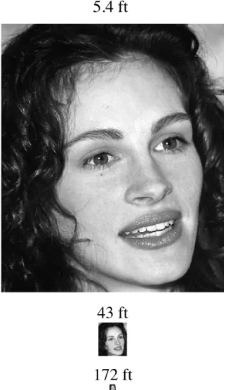
If you ask someone why a face is harder to recognize when it is further away, most people will answer, “be-cause it gets smaller.” This is obviously true in the sense that as a face is moved further from an observer, it shrinks from the observer’s perspective; i.e., its visual angle and retinal size decrease in a manner that is in-versely proportional to distance. So if one wanted to demonstrate the effect of distance on perception, one could do so by appropriately shrinking a picture. This is done in Figure 1, which shows the size that Julia Rob-erts’s face would appear to be, as seen from distances of 5.4, 43, and 172 feet.
The Figure-1 demonstration of the effect of distance on perception is unsatisfying for several reasons. From a practical perspective, it is unsatisfying because (1) its quantitative validity depends on the viewer’s being a specific distance from the display medium (in this in-stance, 22” from the paper on which Figure 1 is printed) and (2) the graininess of the display medium can differ-entially degrade the different-sized images—for in-stance, if one is viewing an image on a computer monitor, an image reduction from, say, 500 x 400 pixels representing a 5-ft distance to 10 x 8 pixels representing a 250-ft distance creates an additional loss of informa-tion, due to pixel reducinforma-tion, above and beyond that re-sulting from simply scaling down the image’s size (and this is true with any real-life display medium: Looking at the bottom image of Figure 1 through a magnifying glass, for instance, will never improve its quality to the point where it looks like the top image). From a scien-tific perspective, the Figure-1 demonstration is unsatis-fying because reducing an image’s size is simply ge-ometry. That is, apart from the basic notion of a retinal image, it does not use any known information about the visual system, nor does it provide any new insight about how the visual system works.
Spatial Frequencies
An alternative to using variation in an image’s size to represent distance is to use variation in the image’s
spatial-frequency composition. It is well known that any image can be represented equivalently in image space and frequency space. The image-space represen-tation is the familiar one: It is simply a matrix of pixels differing in color or, as in the example shown in Figure 1, gray-scale values. The less familiar, frequency-space representation is based on the well known theorem that any two-dimensional function, such as the values of a matrix, can be represented as a weighted sum of sine-wave gratings of different spatial frequencies and ori-entations at different phases (Bracewell, 1986). One can move back and forth between image space and fre-quency space via Fourier transformations and inverse Fourier transformations.
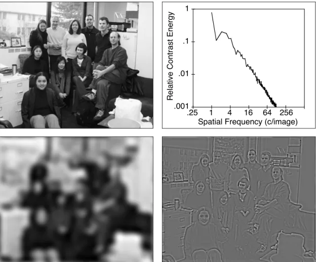
Different spatial frequencies carry different kinds of information about an image. To illustrate, the bottom panels of Figure 2 show the top-left image dichoto-mously partitioned into its low spatial-frequency ponents (bottom left) and high spatial-frequency
com-ponents (bottom right). It is evident that the bottom left picture carries a global representation of the scene, while the bottom-right picture conveys information about edges and details, such as the facial expressions and the objects on the desk. Figure 2 provides an exam-ple of the general princiexam-ple that higher spatial frequen-cies are better equipped to carry information about fine details. In general, progressively lower spatial frequen-cies carry information about progressively coarser fea-tures of the image.
Of interest in the present work is the image’s contrast energy spectrum, which is the function relating contrast energy—informally, the amount of “presence” of some spatial-frequency component in the image—to spatial frequency. For natural images this function declines, and is often modeled as a power function, E = kf
-
r, where E is contrast energy, f is spatial frequency, and k and r are positive constants; thus there is less energy in the higher image frequencies. Figure 2, upper right panel shows this function, averaged over all orienta-tions, for the upper-left image (note that, characteristi-cally, it is roughly linear on a log-log scale). Below, we will describe contrast energy spectra in more detail, in conjunction with our proposed hypothesis about the relation between distance and face processing.Absolute Spatial Frequencies and Image Spatial Frequencies. At this point, we explicate a distinction between two kinds of spatial frequencies that will be critical in our subsequent logic. Absolute spatial fre-quency is defined as spatial frefre-quency measured in cy-cles per degree of visual angle (cycy-cles/deg). Image spa-tial frequency is defined as spaspa-tial frequency measured in cycles per image (cycles/image). Notationally, we will use F to denote absolute spatial frequency (F in cycles/deg), and f to denote image spatial frequency (f in cycles/image).
Note that the ratio of these two spatial frequency measures, F/f in image/deg, is proportional to observer-stimulus distance. Imagine, for instance, a observer-stimulus consisting of a piece of paper, 1 meter high, depicting 10 cycles of a horizontally-aligned sine-wave grating. The image frequency would thus be f = 10 cy-cles/image. If this stimulus were placed at a distance of 57.29 meters from an observer, its vertical visual angle can be calculated to be 1 deg, and the absolute spatial frequency of the grating would therefore be F = 10 cles/1 deg = 10 cycles/deg, i.e., F/f = (10 cy-cles/deg)/(10 cycles/image) = 1 image/deg. If the ob-server-stimulus distance were increased, say by a factor of 5, the visual angle would be reduced to 1/5 = 0.2 deg, the absolute spatial frequency would be increased to F = 10 cycles/0.2 deg = 50 cycles/deg, and F/f = 50/10 = 5 image/deg. If, on the other hand, the distance were decreased, say by a factor of 8, the visual angle would be increased to 1 x 8 = 8 deg, the absolute spatial frequency would be F = 10 cycles/8 deg = 1.25 cy-cles/deg, and F/f = 1/8 image/deg. And so on.
5.4 ft
43 ft
172 ft
Figure 1. Representation of distance by reduction of visual angle. The visual angles implied by the three viewing distances are correct if this page is viewed from a distance of 22”.
Filters, Modulation-Transfer Functions, and Con-trast-Sensitivity Functions. Central to our ideas is the concept of a spatial filter, which is a visual processing device that differentially passes different spatial fre-quencies. A filter’s behavior is characterized by a modulation-transfer function (MTF) which assigns an amplitude scale factor to each spatial frequency. The amplitude scale factor ranges from 1.0 for spatial fre-quencies that are completely passed by the filter to 0.0 for spatial frequencies that are completely blocked by it.
The human visual system can be construed as con-sisting of a collection of components—e.g., the optics of the eye, the receptive fields of retinal ganglion cells, and so on—each component acting as a spatial filter. This collection of filters results in an overall MTF in humans whose measured form depends on the particu-lar physical situation and the particuparticu-lar task in which the human is engaged.
What do we know about the human MTF? In certain
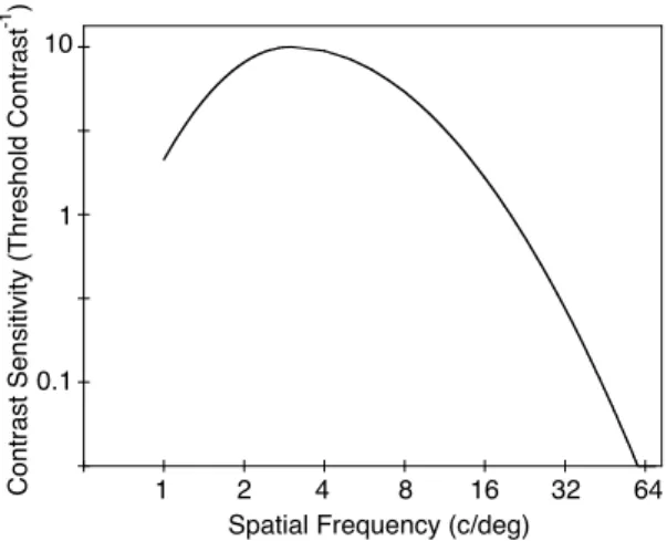
situations, the MTF can be described by a contrast-sensitivity function (CSF) which is the reciprocal of threshold contrast (i.e., contrast sensitivity) as a func-tion of absolute spatial frequency. A “generic” CSF, shown in Figure 3 reasonably resembles those obtained empirically under static situations (e.g., Campbell & Robson, 1968; van Nes & Bouman, 1967). As can be seen, it is band-pass; that is, it best represents spatial frequencies around 3 cycles/deg, while both lower and higher spatial frequencies are represented more poorly. It is the case however, that under a variety of conditions the CSF is low-pass rather than band pass. These con-ditions include low luminance (e.g., van Nes & Bou-man, 1967), high contrast (Georgson & Sullivan, 1975), and temporally varying, rather than static stimuli (e.g., Robson, 1966).
Thus, the form of the CSF under a variety of circum-stances is known. However, measurements of the CSF have been carried out using very simple stimuli, typi-cally sine-wave gratings, under threshold conditions, and its application to suprathreshold complex stimuli
R
elative C
ontrast Energy
.001 .01 .1 1
Spatial Frequency (c/image) 1 4 16 64 256 .25
Figure 2. Decomposition of a naturalistic scene (top left) into low spatial-frequency components (bottom left) and high spatial-frequency components (bottom right). The top right panel shows the contrast energy spectrum of the top-left picture.
such as faces is dubious. One of the goals of the present research is to estimate at least the general form of the relevant MTF for the face-processing tasks with which we are concerned.
Acuity. While measurement of the CSF has been a topic of intense scrutiny among vision scientists, prac-titioners in spatial vision, e.g., optometrists, rely mainly on measurement of acuity. As is known by anyone who has ever visited an eye doctor, acuity measurement en-tails determining the smallest stimulus of some sort—“smallest” defined in terms of the visual angle subtended by the stimulus—that one can correctly identify. Although the test stimuli are typically letters, acuity measurements have been carried out over the past century using numerous stimulus classes including line separation (e.g., Shlaer, 1937), and Landolt C gap size (e.g., Shlaer, 1937). As is frequently pointed out (e.g., Olzak & Thomas, 1989, p. 7-45), measurement of acuity essentially entails measurement of a single point on the human MTF, namely the high-frequency cutoff, under suprathreshold (high luminance and high con-trast) conditions.
The issues that we raised in our Prologue and the re-search that we will describe are intimately concerned with the question of how close a person must be—that is, how large a visual angle the person must sub-tend—to become recognizable. In other words, we are concerned with acuity. However, we are interested in more than acuity for two reasons. First our goals extend beyond simply identifying the average distance at which a person can be recognized. We would like in-stead to be able to specify what, from the visual sys-tem’s perspective, is the spatial-frequency composition of a face at any given distance. Achievement of such goals would constitute both scientific knowledge neces-sary for building a theory of how visual processing de-pends on distance and practical knowledge useful for conveying an intuitive feel for distance effects to inter-ested parties such as juries. Second, it is known that
face processing in particular depends on low and me-dium spatial frequencies, not just on high spatial fre-quencies (e.g., Harmon & Julesz, 1973).
Distance and Spatial Frequencies. Returning to the issue of face perception at a distance, suppose that there were no drop in the MTF at lower spatial frequen-cies—below I will argue that, for purposes of the pre-sent applications, this supposition is plausible. This would make the corresponding MTF low-pass rather than band-pass.
Let us, for the sake of illustration, assume a low-pass MTF that approaches zero around F = 30 cycles/deg (a value estimated from two of the experiments described below); that is, absolute spatial frequencies above 30 cycles/deg can be thought of as essentially invisible to the visual system. Focusing on this 30 cycles/deg upper limit, we consider the following example. Suppose that a face is viewed from 43 feet away, at which distance it subtends a visual angle of approximately 1 deg1. This means that at this particular distance, image frequency f = absolute frequency F, and therefore spatial frequen-cies greater than about f = 30 cycles per face will be invisible to the visual system; i.e., facial details smaller than about 1/30 of the face’s extent will be lost. Now suppose the distance is increased, say by a factor of 4 to 172 feet. At this distance, the face will subtend ap-proximately 1/4 deg of visual angle, and the spatial-frequency limit of F = 30 cycles/deg translates into f = 30 cycles/deg x 1/4 deg/face = 7.5 cycles/face. Thus, at a distance of 172 feet, details smaller than about (1/30)x4 = 2/15 of the face’s extent will be lost. If the distance is increased by a factor of 10 to 430 feet, de-tails smaller than about (1/30)x10 = 1/3 of the face’s extent will be lost And so on. In general, progressively coarser facial details are lost to the visual system in a manner that is inversely proportional to distance.
These informal observations can be developed into a more complete mathematical form. Let the filter corre-sponding to the visual system’s MTF be expressed as,
A = c(F) (1)
where A is the amplitude scale factor, F is frequency in cycles/deg, and c is the function that relates the two. Now consider A as a function not of F, absolute spatial frequency, but of image spatial frequency, f. Because 43 ft is the approximate distance at which a face sub-tends 1 deg, it is clear that f=F*(43/D) where D is the face’s distance from the observer. Therefore, the MTF defined in terms of cycles/face is,
1 In this article, we define face size as face height because our stimuli were less variable in this dimension than in face width. Other studies have defined face size as face width. A face’s height is greater than its width by a factor of approximately 4/3. When we report results for other studies, we transform relevant numbers, where necessary, to reflect face size defined as height.
Contrast S
ensitivity (Threshold Contrast
-1 )
Spatial Frequency (c/deg)
1 2 4 8 16 32 64
0.1 1 10
Figure 3. Band-pass approximation to a human contrast-sensitivity function for a low-contrast, high-luminance, static scene.
†
A
=
c(f )
=
c
43F
D
Ê
Ë
Á
ˆ
¯
˜
(2)Simple though it is, Equation 2 provides, as we shall see, the mathematical centerpiece of much of what fol-lows.
Distance Represented by Filtering. This logic implies an alternative to shrinking a face (Figure 1) as a means of representing the effect of distance. Assume that one knows the visual system’s MTF for a particular set of circumstances, i.e., that one knows the “c” in Equations 1-2. Then to represent the face as seen by an observer at any given distance D, one could remove high image frequencies by constructing a filter as defined by Equa-tion 2 and applying the filter to the face.
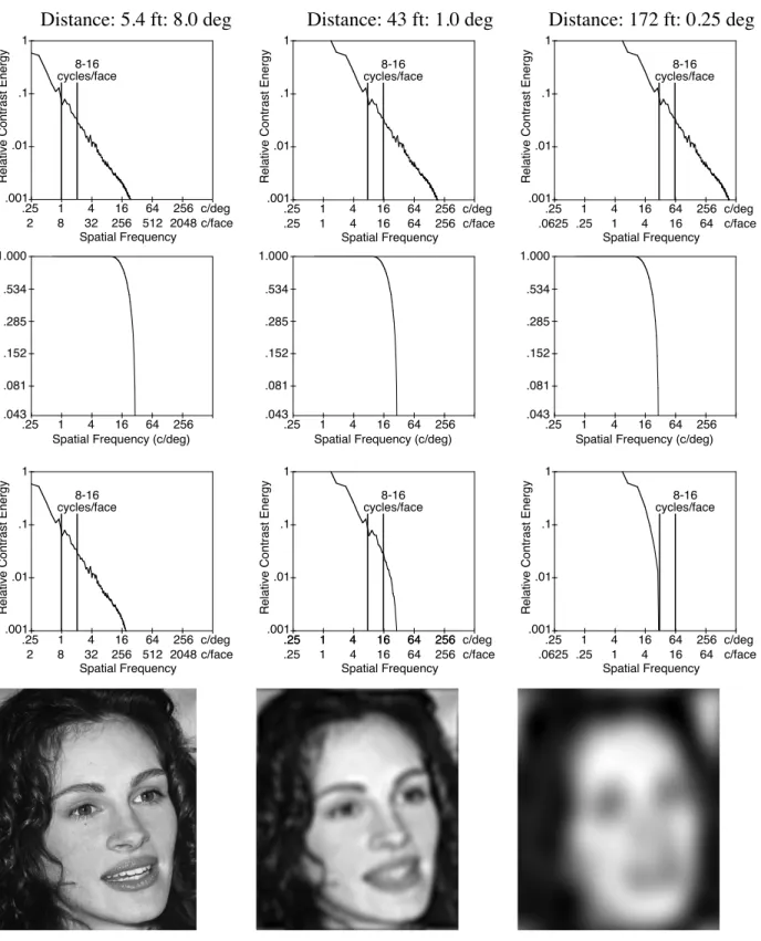
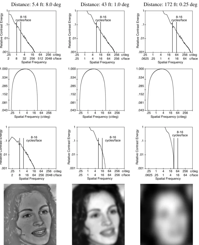
Figure 4 demonstrates how this is done. Consider first the center panels in which Julia Roberts is assumed to be viewed from a distance of D=43 feet away (at which point, recall, F = f). We began by computing the Fourier transform of the original picture of her face. The resulting contrast energy spectrum, averaged over all orientations, is shown in the top center panel (again roughly linear on a log-log scale). Note that the top-row (and third-row) panels of Figure 5 have two abscissa scales: absolute frequency in cycles/deg, and image frequency in cycles/face. To provide a reference point, we have indicated the region that contains between 8 and 16 cycles/face, an approximation of which has been suggested as being important for face recognition (e.g., Morrison & Schyns, 2001). Because at D=43 feet the face subtends, as indicated earlier, 1 deg of visual an-gle, 8-16 cycles/face corresponds to 8-16 cycles/deg. The second row shows a low-pass filter: a candidate human MTF. We describe this filter in more detail be-low, but essentially, it passes absolute spatial frequen-cies perfectly up to 10 cycles/deg and then falls parabolically, reaching zero at 30 cycles/deg. The third row shows the result of filtering which, in frequency space, entails simply multiplying the top-row contrast-energy spectrum by the second-row MTF on a point-by-point basis. Finally, the bottom row shows the result of inverse-Fourier transforming the filtered spectrum (i.e., the third-row spectrum) back to image space. The re-sult—the bottom middle image—is slightly blurred compared to the original (Figure 1) because of the loss of high spatial frequencies expressed in terms of cy-cles/face (compare the top-row, original spectrum to the third-row, filtered spectrum).
Now consider the left panels of Figure 4. Here, Ms. Roberts is presumed to be seen from a distance of 5.4 feet; that is, she has moved closer by a factor of 8 and thus subtends a visual angle of 8 deg. This means that the Fourier spectrum of her face has likewise scaled down by a factor of 8; thus, for instance, the 8-16 cy-cles/face region now corresponds to 1-2 cycles/deg. At this distance, the MTF has had virtually no effect on the
frequency spectrum; that is, the top-row, unfiltered spectrum and the third-row, filtered, spectrum are virtu-ally identical and as a result, the image is unaffected. Finally, in the right panel, Ms. Roberts has retreated to 172 feet away, where she subtends a visual angle of 0.25 deg. Now her frequency spectrum has shifted up so that the 8-16 cycles/face corresponds to 32-64 cy-cles/deg. Because the MTF begins to descend at 10 cycles/deg, and obliterates spatial frequencies greater than 30 cycles/deg, much of the high spatial-frequency information has vanished. The 8-16 cycles/face infor-mation in particular has been removed. As a result, the filtered image is very blurred, arguably to the point that one can no longer recognize whom it depicts.
Rationale for a Low-Pass MTF. To carry out the kind of procedure just described, it was necessary to choose a particular MTF, i.e., to specify the function c in Equations 1-2. Earlier, we asserted that, for present purposes, it is reasonable to ignore the MTF falloff at lower spatial frequencies. As we describe in more detail below, the assumed MTFs used in the calculations to follow are low-pass. There are three reasons for this choice.
Suprathreshold Contrast Measurements. Although there are numerous measurements of the visual sys-tem’s threshold CSF, there has been relatively little research whose aim is to measure the suprathreshold CSF. One study that did report such work was reported by Georgeson and Sullivan (1975). They used a matching paradigm in which observers adjusted the perceived contrast of a comparison sine-wave grating shown at one of a number of spatial frequencies to the perceived contrast of a 5 cycles/deg test grating. They found that at low contrasts, the resulting functions re-lating perceived contrast to spatial frequency were bandpass. At higher contrast levels (beginning at a contrast of approximately 0.2) the functions were ap-proximately flat between 0.25 and 25 cycles/deg which were the limits of the spatial-frequency values that the authors reported.
Absolute versus Image Frequency: Band-Passed Faces at Different Viewing Distances. Several experiments have been reported in which absolute and image spatial frequency have been disentangled using a design in which image spatial frequency and observer-stimulus distance—which influences absolute spatial fre-quency—have been factorially varied (Parish & Sper-ling, 1991; Hayes, Morrone, and Burr 1986). Generally these experiments indicate that image frequency is im-portant and robust in determining various kinds of task performance, while absolute frequency makes a differ-ence only with high image frequencies.
To illustrate the implication of such a result for the shape of the MTF, consider the work of Hayes et al. who reported a face-identification task: Target faces,
Distance: 5.4 ft: 8.0 deg
Distance: 43 ft: 1.0 deg
Distance: 172 ft: 0.25 deg
Relative Contrast Energy
.001 .01 .1 1
Spatial Frequency
1 4 16 64 256
.25 c/deg
8-16 cycles/face
8 32 256 512 2048
2 c/face
8-16 cycles/face
Relative Contrast Energy
.001 .01 .1 1
Spatial Frequency
1 4 16 64 256
.25 c/deg
1 4 16 64 256
.25 c/face
8-16 cycles/face
Relative Contrast Energy
.001 .01 .1 1
Spatial Frequency 1 4 16 64 256
.25 c/deg
.25 1 4 16 64
.0625 c/face
.043 .081 .152 .285 .534 1.000
Spatial Frequency (c/deg) 1 4 16 64 256
.25 .043
.081 .152 .285 .534 1.000
Spatial Frequency (c/deg) 1 4 16 64 256
.25 .043
.081 .152 .285 .534 1.000
Spatial Frequency (c/deg) 1 4 16 64 256 .25
8-16 cycles/face
Relative Contrast Energy
.001 .01 .1 1
Spatial Frequency
1 4 16 64 256
.25 c/deg
8 32 256 512 2048
2 c/face
1 4 16 64 256
.25
8-16 cycles/face
Relative Contrast Energy
.001 .01 .1 1
Spatial Frequency
1 4 16 64 256
.25 c/deg
1 4 16 64 256
.25 c/face
8-16 cycles/face
Relative Contrast Energy
.001 .01 .1 1
Spatial Frequency 1 4 16 64 256
.25 c/deg
.25 1 4 16 64
.0625 c/face
Figure 4. Demonstration of low-pass filtering and its relation to distance. The columns represent 3 distances rang-ing from 5.4 to 172 ft. Top row: contrast energy spectrum at the 3 distances (averaged across orientations). Second row: Assumed low-pass MTF corresponding to the human visual system. Third row: Result of multiplying the filter by the spectrum: With longer distances, progressively lower image frequencies are eliminated. Bottom row: Filtered images—the phenomenological appearances at the various distances—that result.
band-passed at various image frequencies were pre-sented to observers who attempted to identify them. The band-pass filters were 1.5 octaves wide and were centered at one of 5 image-frequency values ranging from 4.4 to 67 cycles/face. The faces appeared at one of two viewing distances, differing by a factor of 4—which, of course, means that the corresponding ab-solute spatial frequencies also differed by a factor of 4. Hayes at al. found that recognition performance de-pended strongly on image frequency, but dede-pended on viewing distance only with the highest image-frequency filter, i.e., the one centered at 67 cycles/face. This filter passed absolute spatial frequencies from approximately 1.7 to 5.0 cycles/deg for the short viewing distance and from approximately 7 to 20 cycles/deg for the long viewing distance. Performance was better at the short viewing distance corresponding to the lower absolute spatial-frequency range, than at the longer distance, corresponding to the higher absolute spatial-frequency range. The next highest filter, which produced very little viewing-distance effect passed absolute spatial frequencies from approximately 0.9 to 2.5 cycles/deg for the short long viewing distance and from approxi-mately 3.5 to 10 cycles/deg for the long viewing dis-tance.
These data can be explained by the assumptions that (1) performance is determined by the visual system’s representation of spatial frequency in terms of cy-cles/face and (2) the human MTF in this situation is low-pass—it passes absolute spatial frequencies per-fectly up to some spatial frequency between 10 and 20 cycles/deg before beginning to drop. Thus, with the second-highest filter the perceptible frequency range would not be affected by the human MTF at either viewing distance. With the highest filter, however the perceptible frequency range would be affected by the MTF at the long, but not at the short viewing distance.
Phenomenological Considerations. Suppose that the suprathreshold MTF were band-pass as in Figure 3. In that case, we could simulate what a face would look like at varying distances, just as we described doing earlier using a low-pass filter. In Figure 5, which is organized like Figure 4, we have filtered Julia Roberts’ face with a band-pass filter, centered at 3 cycles/deg. It is constructed such that falls to zero at 30 cycles/deg just as does the Figure-4 low-pass filter, but also falls to zero at 0.2 cycles/deg. For the 43- and 172-ft distances, the results seem reasonable—the filtered images are blurred in much the same way as are the Figure-4, low-passed images. However, the simulation of the face as seen from 5.4 ft is very different: It appears band-passed. This is, of course, because it is band passed, and at a distance as close as 5.4 ft, the band-pass nature of the filter begins to manifest itself. At even closer dis-tances, the face would begin to appear high-passed, i.e., like the Figure-2 bottom-right picture. The point is that simulating distance using a band-pass filter yields rea-sonable phenomenological results for long simulated
distances, but at short simulated distances, yields im-ages that look very different than actual objects seen close up. A low-pass filter, in contrast, yields images that appear phenomenologically reasonable at all virtual distances.
The Distance-As-Filtering Hypothesis
We will refer to the general idea that we have been describing as the distance-as-filtering hypothesis. Spe-cifically, the distance-as-filtering hypothesis is the conjunction of the following two assumptions.
1. The difficulty in perceiving faces at increasing dis-tances comes about because the visual system’s limita-tions in representing progressively lower image fre-quencies, expressed in terms of cycles/face, causes loss of increasingly coarser facial details.
2. If an appropriate MTF, c (see Equations 1-2 above) can be determined, then the representation of a face viewed from a particular distance, D, is equivalent to the representation acquired from the version of the face that is filtered in accord with Equation 2.
The Notion of “Equivalence”. Before proceeding, we would like to clarify what we mean by “equivalent.” There are examples within psychology wherein physi-cally different stimuli give rise to representations that are genuinely equivalent at any arbitrary level of the sensory-perceptual-cognitive system, because the in-formation that distinguishes the stimuli is lost at the first stage of the system. A prototypical example is that of color metamers—stimuli that, while physically dif-ferent wavelength mixtures, engender identical quan-tum-catch distributions in the photoreceptors. Because color metamers are equivalent at the photoreceptor stage, they must therefore be equivalent at any subse-quent stage.
When we characterize distant and low-pass filtered faces as “equivalent” we do not, of course mean that they are equivalent in this strong sense. They are not phenomenologically equivalent: One looks small and clear; the other looks large and blurred; and they are obviously distinguishable. One could, however, propose a weaker definition of “equivalence.” In past work, we have suggested the term “informational metamers” in reference to two stimuli that, while physically and phe-nomenologically different, lead to presumed equivalent representations with respect to some task at hand (see Loftus & Ruthruff, 1994; Harley, Dillon, & Loftus, in press). For instance Loftus, Johnson, & Shimamura (1985) found that a d-ms unmasked stimulus (that is a stimulus plus an icon) is equivalent to a (d+100)-ms masked stimulus (a stimulus without an icon) with respect to subsequent memory performance across a wide range of circumstances. Thus it can be argued that the representations of these two kinds of physically and phenomenologically different stimuli eventually con-verge into equivalent representations at some point prior to whatever representation underlies task performance.
Similarly, by the distance-as-filtering hypothesis we propose that reducing the visual angle of the face on the one hand, and appropriately filtering the face on the
other hand lead to representations that are equivalent in robust ways with respect to performance on various tasks. In the experiments that we report below, we
con-Distance: 5.4 ft: 8.0 deg
Distance: 43 ft: 1.0 deg
Distance: 172 ft: 0.25 deg
Relative Contrast Energy
.001 .01 .1 1
Spatial Frequency
1 4 16 64 256
.25 c/deg
8-16 cycles/face
8 32 256 512 2048
2 c/face
8-16 cycles/face
Relative Contrast Energy
.001 .01 .1 1
Spatial Frequency 1 4 16 64 256
.25 c/deg
1 4 16 64 256
.25 c/face
8-16 cycles/face
Relative Contrast Energy
.001 .01 .1 1
Spatial Frequency 1 4 16 64 256
.25 c/deg
.25 1 4 16 64
.0625 c/face
Spatial Frequency (c/deg)
1 4 16 64 256
.25 .043 .081 .152 .285 .534 1.000
Spatial Frequency (c/deg)
1 4 16 64 256
.25 .043 .081 .152 .285 .534 1.000
Spatial Frequency (c/deg) 1 4 16 64 256 .25
.043 .081 .152 .285 .534 1.000
8-16 cycles/face
Relative Contrast Energy
.001 .01 .1 1
Spatial Frequency
1 4 16 64 256
.25 c/deg
c/face
8 16 64 256 2048
2
Relative Contrast Energy
.001 .01 .1 1
Spatial Frequency 1 4 16 64 256
.25 c/deg
c/face 8-16 cycles/face
1 4 16 64 256 .25
8-16 cycles/face
Relative Contrast Energy
.001 .01 .1 1
Spatial Frequency
1 4 16 64 256
.25 c/deg
c/face
.25 1 4 16 64
.0625
Figure 5. Demonstration of band-pass filtering and its relation to distance. This figure is organized like Figure 4 ex-cept that the visual system’s MTF assumed is, as depicted in the second-row panels, band-pass rather than low-pass.
firm such equivalence with two tasks.
Different Absolute Spatial-Frequency Channels?
A key implication of the distance-as-filtering hypothe-sis is that the visual system’s representation of a face’s image frequency spectrum is necessary and sufficient to account for distance effects on face perception: That is, two situations—a distant (i.e., small retinal image) un-filtered face and a closer (i.e., large retinal image) suitably filtered face will produce functionally equiva-lent representations and therefore equal performance.
Note, however that for these two presumably equivalent stimuli, the same image frequencies corre-spond to different absolute frequencies: They are higher for the small unfiltered face than for the larger filtered face. For instance, a test face sized to simulate a dis-tance of 108 ft would subtend a visual angle of ap-proximately 0.40 deg. A particular image spatial fre-quency—say 8 cycles/face—would therefore corre-spond to an absolute spatial frequency of approximately 20 cycles/deg. A corresponding large filtered face, however, subtends, in our experiments, a visual angle of approximately 20 deg, so the same 8 cycles/face would correspond to approximately 0.4 cycles/deg.
There is evidence from several different paradigms that the visual system decomposes visual scenes into separate spatial frequency channels (Blakemore & Campbell, 1969; Campbell & Robeson, 1968 Graham, 1989; Olzak & Thomas, 1986; De Valois & De Valois, 1980; 1988). If this proposition is correct it would mean that two presumably equivalent stimulus representa-tions—a small unfiltered stimulus on the one hand and a large filtered stimulus on the other—would issue from different spatial frequency channels. One might expect that the representations would thereby not be equivalent in any sense, i.e., that the distance-as-filtering hypothe-sis would fail under experimental scrutiny. As we shall see, however, contrary to such expectation, the hy-pothesis holds up quite well.
General Prediction. With this foundation, a general prediction of the distance-as-filtering hypothesis can be formulated: It is that in any task requiring visual face processing, performance for a face whose distance is simulated by appropriately sizing it will equal perform-ance for a face whose distperform-ance is simulated by appro-priately filtering it.
EXPERIMENTS
We report four experiments designed to test this gen-eral prediction. In Experiment 1, observers matched the informational content of a low-pass-filtered comparison stimulus to that of a variable-sized test stimulus. In Ex-periments 2-4, observers attempted to recognize pic-tures of celebrities that were degraded by either low-pass filtering or by size reduction.
Experiment 1: Matching Blur to Size
Experiment 1 was designed to accomplish two goals. The first was to provide a basic test of the distance-as-filtering hypothesis. The second goal, given reasonable accomplishment of the first, was to begin to determine the appropriate MTF for representing distance by spa-tial filtering. In quest of these goals a matching para-digm was devised. Observers viewed an image of a test face presented at one of six different sizes. Each size corresponded geometrically to a particular observer-face distance, D, that ranged from 20 to 300 ft. For each test size, observers selected which of 41 progressively more blurred comparison faces best matched the per-ceived informational content of the test face.
The set of 41 comparison faces was constructed as follows. Each comparison face was generated by low-pass filtering the original face using a version of Equa-tion 2 to be described in detail below. Across the 41 comparison faces the filters removed successively more high spatial frequencies and became, accordingly, more and more blurred. From the observer’s perspective, these faces ranged in appearance from completely clear (when the filter’s spatial-frequency cutoff was high and it thereby removed relatively few high spatial frequen-cies) to extremely blurry (when the filter’s spatial-frequency cutoff was low and it thereby removed most of the high spatial frequencies). For each test-face size, the observer, who was permitted complete, untimed access to all 41 comparison faces, selected the particu-lar comparison face that he or she felt best matched the perceived informational content of the test face. Thus, in general, a large (simulating a close) test face was matched by a relatively clear comparison face, while a smaller (simulating a more distant) test face was matched by a blurrier comparison face.
Constructing the Comparison Faces. In this section, we provide the quantitative details of how the 41 filters were constructed in order to generate the corresponding 41 comparison faces.
We have already argued that a low-pass filter is ap-propriate as a representation of the human MTF in this situation and thus as a basis for the comparison pictures to be used in this task. A low-pass filter can take many forms. Somewhat arbitrarily, we chose a filter that is constant at 1.0 (which means it passes spatial frequen-cies perfectly) up to some rolloff spatial frequency, termed F0 cycles/deg, then declines as a parabolic func-tion of log spatial frequency, reaching zero at some cutoff spatial frequency, termed F1 cycles/deg, and re-maining at zero for all spatial frequencies greater than F1. We introduce a constant, r > 1, such that F0=F1/r. Note that r can be construed as the relative slope of the filter function: lower r values correspond to steeper slopes.
Given this description, for absolute spatial frequen-cies defined in terms of F, cycles/deg, the filter is com-pletely specified and is derived to be,
c(F) =
†
1.0 for F < F0
1- log(F/F0)
log(r)
È Î
Í ˘
˚ ˙ 2
for F0 £F
0.0 for F > F1 Ï
Ì Ô Ô
Ó Ô Ô
£ F1 (3)
Above, we noted that image spatial frequency ex-pressed in terms of f, frequency in cycles/face, is f=(43/D)*F where D is the observer’s distance from the face. Letting k=(43/D), the Equation-3 filter expressed in terms of f is,
c(f, d) =
†
1.0 for f < kF0 1- log(f/kF0)
log(r) È Î Í
˘ ˚ ˙
2
for kF0 £f£ kF1 0.0 for f > kF1
Ï Ì Ô Ô
Ó Ô Ô
(4)
In Equation 4, kF0 and kF1 correspond to what we term f0 and f1 which are, respectively, the rolloff and cutoff frequencies, defined in terms of cycles/face.
Because this was an exploratory venture, we did not know what value of r would be most appropriate. For that reason, we chose two somewhat arbitrary values of r: 3 and 10. The 41 comparison filters constructed for each value of r were selected to produce corresponding images having, from the observer’s perspective, a large range from very clear to very blurry. Expressed in terms of cutoff frequency in cycles/face (f1), the ranges were from 550 to 4.3 cycles/face for the r=10 comparison filters, and from 550 to 5.2 cycles/face for the r=3 com-parison filters. Each comcom-parison image produced by a comparison filter was the same size as the original im-age (1,100 x 900 pixels).
To summarize, each comparison face was defined by a value of f1. On each experimental trial, we recorded the comparison face, i.e., that value of f1 that was se-lected by the observer as matching the test face dis-played on that trial. Thus, the distance corresponding to the size of the test face was the independent variable in the experiment, and the selected value of f1 was the dependent variable.
Prediction. Given our filter-construction process, a candidate MTF is completely specified by values of r and F1. As indicated, we selected two values of r, 3 and 10. We allowed the cutoff frequency, F1, to be a free parameter estimated in a manner to be described below.
Suppose that the distance-as-filtering hypothesis is correct—that seeing a face from a distance is indeed equivalent to seeing a face whose high image frequen-cies have been appropriately filtered out. In that case, a test face sized to subtend a visual angle corresponding to some distance, D, should be matched by a
compari-son face filtered to represent the same distance. As specified by Equation 2 above, f1 = (43F1)/D, or
†
D=43F1
f1
(5)
which means that,
†
1
f
1=
1
43F
1Ê
Ë
Á
Á
ˆ
¯
˜
˜
D
(6)Equation 6 represents our empirical prediction: The measured value of 1/f1 is predicted to be proportional to the manipulated value of D with a constant of propor-tionality equal to 1/(43F1). Given that Equation 6 is confirmed, F1—and thus, in conjunction with r, the MTF as a whole—can be estimated by measuring the slope of the function relating 1/f1 to D, equating the slope to 1/(43F1), solving for F1, and plugging the re-sulting F1 value into Equation 3.
Method
Observers. Observers were 24 paid University of Wash-ington students with normal or corrected-to-normal vision.
Apparatus. The experiment was executed in MATLAB using the Psychophysics Toolbox (Brainard, 1997; Pelli, 1997). The computer was a Macintosh G4 driving two Apple 17” Studio Display monitors. One of the monitors (the near monitor), along with the keyboard, was placed at a normal viewing distance, i.e., approximately, 1.5 ft from the observer. It was used to display the filtered pictures. The other monitor (the far monitor) was placed 8 ft away and was used to dis-play the pictures that varied in size. The resolution of both monitors was set to 1600 x 1200 pixels. The far monitor’s distance from the observer was set so as to address the reso-lution problem that we raised earlier, i.e., to allow shrinkage of a picture without concomitantly lowering the effective resolution of the display medium: From the observer’s per-spective, the far monitor screen had a pixel density of ap-proximately 224 pixels per deg of visual angle thereby ren-dering it unlikely that the pixel reduction associated with shrinking would be perceptible to the observer.
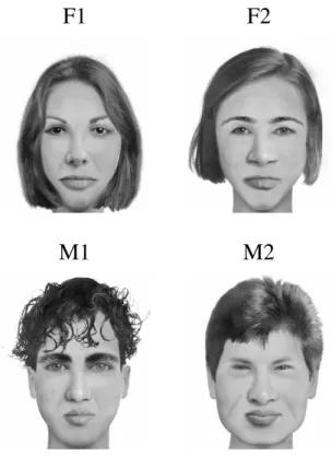
Materials. Four faces, 2 males and 2 females, created us-ing the FACES “Identikit” program were used as stimuli. They are shown in Figure 6. Each face was rendered as a 1,100 x 900 pixel grayscale image, luminance-scaled so that the grayscale values ranged from 0 to 255 across pixels. For each of the 4 faces, six test images were created. They were sized such that, when presented on the far monitor, their vis-ual angles would, to the observer seated at the near monitor, equal the visual angles subtended by real faces seen from 6 test distances: 21, 36, 63, 108, 185, and 318 ft.
Design and Procedure. Each observer participated in 8 consecutive sessions, each session involving one combination of the 4 faces x 2 filter classes (r=3 and r=10). The 8 faces x filter class combinations occurred in random order, but were counterbalanced such that over the 24 observers each combi-nation occurred exactly 3 times in each of the 8 sessions. Each
session consisted of 10 replications. A replication consisted of 6 trials, each trial involving one of the 6 test distances. Within each replication, the order of the 6 test distances was randomized.
On each trial, the following sequence of events occurred. First the test picture was presented on the far screen where it remained unchanged throughout the trial. Simultaneously, a randomly selected one of the 41 comparison faces appeared on the near screen. The observer was then permitted to move freely back and forth through the sequence of comparison faces, all on the near screen. This was done using the left and right arrow keys: Pressing the left arrow key caused the ex-isting comparison image to be replaced by the next blurrier image, whereas pressing the right arrow key produced the next clearer image. All of the 41 comparison faces were held in the computer’s RAM and could be moved very quickly in and out of video RAM, which meant that moving back and forth through the comparison faces could be done very quickly. If either arrow key was pressed and held, the com-parison image appeared to blur or deblur continuously, and to transit through the entire sequence of 41 comparison faces from blurriest to clearest or vice-versa took approximately a second. Thus, the observer could carry out the comparison process easily, rapidly, and efficiently.
As noted earlier, the observer’s task was to select the com-parison stimulus that best matched the perceived informa-tional content of the test stimulus. In particular, the following instructions were provided: “On each trial, you will see what we call a distant face on the far monitor (indicate). On the near monitor, you will have available a set of versions of that face that are all the same size (large) but which range in clar-ity. We call these comparison faces. We would like you to select the one comparison face that you think best matches how well you are able see the distant face.” The observer was
provided unlimited time to do this on each trial, could roam freely among the comparison faces, and eventually indicated his or her selection of a matching comparison face by pressing the up arrow. The response recorded on each trial was the cutoff frequency, f1 in cycles/face, of the filter used to gener-ated the matching comparison face.
Results. Recall that the prediction of the distance-as-filtering hypothesis is that 1/f1 is proportional to size-defined distance, D (see Equation 6). Our first goal was to test this prediction for each of our filter classes, r=3 and r=10. To do so, we calculated the mean value, of 1/f1, across the 24 observers and 4 faces for each value of D. Figure 7 shows mean 1/f1 as a function of D for both r values, along with best-fitting linear functions. It is clear that the curves for both r values are approxi-mated well by zero-intercept linear functions, i.e., by proportional relations. Thus the prediction of the dis-tance-as-filtering hypothesis is confirmed.
Given confirmation of the proportionality prediction, our next step is to estimate the human MTF for each value of r. To estimate the MTF, it is sufficient to esti-mate the cutoff value, F1. which is accomplished by computing the best-fitting zero-intercept slope2 of each of the two Figure-7 functions, equating each of the slope values to 1/(43F1), the predicted proportionality constant, and solving for F1 (again see Equation 6). These values are 52 and 42 cycles/deg for measure-ments taken from stimuli generated by the r=10 and r=3 filters respectively. Note that the corresponding esti-mates of the rolloff frequency F0—the spatial frequency at which the MTF begins to descend from 1.0 enroute to reaching zero at F1—are approximately 5 and 14
2
It can easily be shown that the best-fitting zero-intercept slope of Y against X in an X-Y plot is estimated as SXY/SX2. In this instance, the estimated zero-intercept slopes were almost identical to the un-constrained slopes.
F1
F2
M1
M2
Figure 6. Faces used in Experiment 1.
0.000 0.033 0.067 0.100 0.133 0.167 0.200
0 100 200 300
r=10 r=3
1
/f 1
(fa
ce
/cycle
)
D = Distance Defined by Shrinking (ft) 15.0
7.5 5.0
f1
(cycle
s/fa
ce
)
∞
6.0
10.0
30.0
Figure 7. Experiment-1 results: Reciprocal of measured f1 values (left-hand ordinate) plotted
against distance, D. Right-hand ordinate shows f1
val-ues. Solid lines are best linear fits. Each data point is based on 960 observations. Error bars are standard errors.
cycles/deg for the r=10 and r=3 filters.
Is there any basis for distinguishing which of the two filters is better as a representation of the human MTF? As suggested by Figure 7, we observed the r=3 filter to provide a slightly higher r2 value than the r=10 filter (0.998 versus 0.995). Table 1 provides additional F1 statistics for the two filter classes. Table 1, Column 2 shows the mean estimated F1 for each of the 4 individ-ual faces, obtained from data averaged across the 24 observers. Columns 3-6 show data based on estimating F1 for each individual observer-face-filter combination and calculating statistics across the 24 observers. The Table-1 data indicate, in two ways, that the r=3 filter is more stable than the r=10 filter. First, the rows marked “SD” in Columns 2-4 indicate that there is less vari-ability across faces for the r=3 filter than for the r=10 filter. This is true for F1 based on mean data (Column 2) and for the median and mean of the F1 values across the individual faces (Columns 3-4). Second, Columns 5-6 show that there is similarly less variability across the 24 observers for the r=3 than for the r=10 filter. Finally the difference between the median and mean was smaller for the r=3 than for the r=10 filter, indicating a more symmetrical distribution for the former.
Given that stability across observers and materials, along with distributional symmetry indicates superior-ity, these data indicate that the r=3 filter is the better candidate for representing the MTF in this situation. Our best estimate of the human MTF for our Experi-ment-1 matching task is therefore, F0 = 14, and F1 = 42. We note that these are not the values used to create
Figure 4; the filter used for the Figure-4 demonstrations were derived from Experiments 2-4 which used face recognition.
Discussion. The goal of Experiment 1 was to determine the viability of the distance-as-filtering hypothesis. By this hypothesis, the deleterious effect of distance on face perception is entirely mediated by the loss of pro-gressively lower image frequencies, measured in cy-cles/face, as the distance between the face and the ob-server increases. The prediction of this hypothesis is that, given the correct filter corresponding to the human MTF in a face-perception situation, a face shrunk to correspond to a particular distance D is spatially fil-tered, from the visual system’s perspective in a way that is entirely predictable. This means that if a large-image face is filtered in exactly the same manner, it should be matched by an observer to the shrunken face; i.e., the observer should conclude that the shrunken face and the appropriately filtered large face look alike in the sense of containing the same spatial information.
Because there are not sufficient data in the existing literature, the correct MTF is not known, and this strong prediction could not be tested. What we did instead was to postulate two candidate MTFs and then estimate their parameters from the data. The general prediction is that the function relating the reciprocal of measured filter cutoff frequency, 1/f1 should be proportional to D, dis-tance defined by size. This prediction was confirmed for both candidate MTFs as indicated by the two func-tions shown in Figure 7. Although the gross fits to the data were roughly the same for the two candidate
Table 1
Filter cutoff frequencies (F1 ) statistics for two filter classes(r=10 and r=3) and the four faces
(2 males, M1 and M2, and 2 females, F1 and F2).
Computed across observers
r = 10
Filter Face Mean based onaveraged data Median Mean SD Range
M1 51.0 50.5 60.0 27.1 119
M2 54.7 61.9 60.7 19.5 74
F1 53.1 53.3 57.2 17.6 70
F2 48.0 51.8 54.6 18.1 79
Means 51.7 54.4 58.1 20.6 85.5
SD’s 2.5 4.5 2.4
r = 3
Filter Face
Mean based on
averaged data Median Mean SD Range
M1 44.3 44.9 46.8 14.0 53
M2 45.7 46.1 46.0 11.0 46
F1 41.3 43.1 42.7 10.6 43
F2 40.5 40.1 42.3 9.8 34
Means 42.9 43.6 44.5 11.3 44.0
SD’s 2.1 2.3 2.0
Note—In the rows labeled “Means” and “SD’s”, each cell contains the mean or standard deviations of the 4 numbers imme-diately above it; i.e., they refer to statistics over the 4 faces for each filter class. The columns labeled “Mean”, “Standard De-viation” and “Range” refer to statistics computed over the 24 observers
MTFs—they were both excellent—a criterion of con-sistency over observers and stimuli weighed in favor of the r=3 filter over the r=10 filter. We reiterate that our estimated r=3 filter, in combination with a F1 value of 42 cycles/deg, implies a MTF that passes spatial fre-quencies perfectly up to 14 cycles/deg and then falls, reaching zero at 42 cycles/deg.
How does this estimate comport with past data? The Georgeson & Sullivan data discussed earlier indicated a fairly flat human suprathreshold MTF up to at least 25 cycles/deg which is certainly higher than the 14 cy-cles/deg rolloff frequency that we estimate here. Georgeson and Sullivan used a different task from the present one: Their observers adjusted contrast of sine-wave gratings of specific spatial frequencies to match a 5 cycles/deg standard, while the present observers matched spatial-frequency composition of constant-contrast faces to match different-size test stimuli. Be-cause their highest comparison grating was 25 cy-cles/deg, we do not know if and how the function would have behaved at higher spatial frequencies. Similarly, the present measurements of MTF shape are limited because we used only r values of 3 and 10. It is possible that if, for instance, we had used an r=2 filter, we would have estimated a larger rolloff frequency.
Our estimated MTF shape does accord well with data described earlier reported by Hayes et al. (1986). They reported an experiment in which faces were (1) filtered with band-pass filters centered at difference image fre-quencies (expressed in terms of cycles/face), and (2) presented at different viewing distances which, for a given image-frequency distribution, affected the distri-bution of absolute spatial frequencies (expressed in cycles/deg). As we articulated earlier, Hayes et al.’s data can be nicely accommodated with the assumptions that (1) the human MTF is low-pass for their experi-ment, and (2) it passed spatial frequencies perfectly up to somewhere between 10 and 20 cycles/deg.
In Experiments 2-4 we explore whether the MTF fil-ter estimated from the matching task used in Experi-ment 1 is also appropriate for face identification. To anticipate, the filter that we estimate in Experiments 2-4 has smaller values of F0 and F1; i.e., it is scaled toward lower spatial frequencies. In our General Discussion, we consider why that may happen. For the moment we note that one common observer strategy in Experiment 1 was to focus on small details (e.g., a lock of hair), judge how visible that detail was in the distant face, and then adjust the comparison face so that it was equally visible. This focusing on small details may mean that the observers in Experiment 1 may have viewed their task as more like looking at an eye chart than a face, and that whatever processes are “special” to face proc-essing were minimized in Experiment 1. In Experi-ments 2-4 we dealt with the same general issues as in Experiment 1, but using a task that is unique to face processing—recognition of known celebrities.
Experiment 2: Celebrity Recognition at a
Dis-tance—Priming
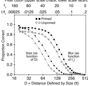
Experiments 2-4 used the same logic as Experiment 1, relating distance defined by low-pass spatial filtering to distance defined by size. However, the stimuli, task, and dependent variables were all very different. On each of a series of trials in Experiments 2-4, observers identified a picture of a celebrity. The picture began either very small or very blurry—so small or blurry as to be entirely unrecognizable—and then gradually clari-fied by either increasing in size or deblurring. The ob-server’s mission was to identify the celebrity as early as possible in this clarification process, and the clarity point at which the celebrity was correctly identified was recorded on each trial. This clarity point was charac-terized as the distance implied by size, D, in the case of increasing size, and as filter cutoff frequency in cy-cles/face, f1, in the case of deblurring. As in Experiment 1, the central prediction of the distance-as-filtering hy-pothesis is that 1/f1 is proportional to D with a propor-tionality constant of 1/(43F1). Again as in Experiment 1, given confirmation of this prediction, F1 can be esti-mated by equating the observed constant of proportion-ality to 1/(43F1) and solving for F1.
Given confirmation of the prediction, it becomes of interest to determine how robust is the estimate of the human MTF. We evaluated such robustness in two ways. The first was to compare the MTF estimates based on recognition (Experiments 2-4) with the esti-mate based on matching (Experiment 1). The second was to compare MTF estimates within each of Experi-ments 2-4 under different circumstances. In particular, in each of Experiments 2-4, we implemented a di-chotomous independent variable that, it was assumed based on past data, would affect identification perform-ance. The variable was “cognitive” or “top-down” in that variation in it did not affect any physical aspect of the stimulus; rather it affected only the observer’s ex-pectations or cognitive strategies. The purpose of incor-porating these variables was to test substitutability of the presumed human MTF (Palmer, 1986a; 1986b; see also Bamber, 1979). The general idea of substitutability is that some perceptual representation, once formed, is unaffected by variation in other factors; i.e., substitut-ability implies a kind of independence. The distance-as-filtering hypothesis is that distance-as-filtering a face by some specified amount produces a perceptual representation that is functionally equivalent to the representation that is obtained when the face is viewed from a distance. Addition of the stronger substitutability hypothesis is that this equivalence is unaffected by changes in other, nonperceptual variables. Therefore the prediction of substitutability is that the same MTF—i.e., the same estimated value of F1—should describe the relation between distance defined by size and distance defined by filtering for both levels of the cognitive variable.
Half of the to-be-identified celebrities had been primed in that the observer had seen their names a few minutes prior to the identification part of the experiment. The other half of the to-be-identified celebrities had not been primed. Numerous past studies (e.g., Reinitz & Alexander, 1996; Tulving & Schacter, 1990) have indi-cated that such priming improves eventual recognition of the primed stimuli.
Method
Observers. Observers were 24 paid University of Wash-ington graduates and undergraduates with normal, or cor-rected-to-normal vision. All were raised in the United States, and professed reasonable familiarity with celebrities, broadly defined.
Apparatus. Apparatus was the same as that used in Ex-periment 1.
Materials. Pictures of 64 celebrities were obtained from various sources, principally the internet and glossy maga-zines. The celebrities came from all walks of celebrity life. They included actors, musicians, politicians, business figures, and sports figures, chosen so as to be recognizable by as many potential observers as possible. There were 43 males and 21 females. They were all rendered initially as grayscale images. They were scaled to be 500 pixels high, but varied in width. Each image was luminance-scaled so as to range in grayscale level from 0 to 255 across pixels.
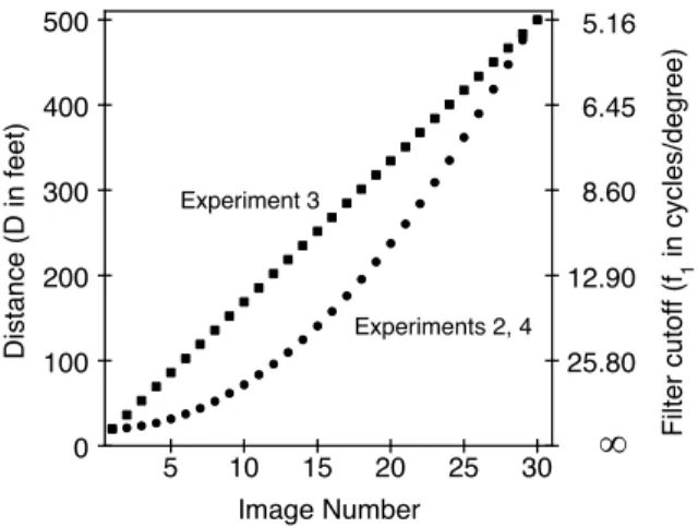
Beginning with a single original photograph of each celeb-rity, two 30-image sets were created. Images in the first set varied in size such that, when shown on the far monitor, they subtended visual angles corresponding to distances ranging from 20 to 500 ft. Images in the second set were filtered using the r=3 filter class described in conjunction with Experiment 1. The cutoff values, f1, ranged from 129 to 5.2 cycles/face. The exact function relating degree of degradation to degrada-tion image number (1-30) was somewhat complex and repre-sented an attempt to make the transition from one degraded image to the next less degraded image as perceptually similar as possible across all 30 degraded images for both the size-increase and the deblurring procedures, The function is shown by the circles in Figure 8. The left ordinate refers to degrada-tion defined in terms of size reducdegrada-tion (distance D) while the right ordinate refers to degradation defined in terms of filter-ing (cutoff frequency1/f1; note the reciprocal scale). Sizes of the filtered images were the same as sizes of the original im-ages (500 pixels high x variable widths).
Design and Counterbalancing.Observers were run indi-vidually. Each observer participated in 4 blocks of 16 tri-als/block. Each trial involved a single celebrity whose image clarified by either increasing in size or by deblurring. All trials within a block involved just one clarification type, in-creasing in size or deblurring. For half the observers the Blur (B) and Size (S) block sequence was BSSB while for the other half, the sequence was SBBS. Within each block, half the celebrities had been primed in a manner to be described shortly, whereas the other half the celebrities had not been primed.
Each observer had a “mirror-image” counterpart whose trial sequence was identical except that primed-unprimed was reversed. Therefore, 4 observers formed a complete counter-balancing module, and the 24 observers comprised 6 such
modules. The order of the 64 celebrities across trials was constant across the 4 observers within each counterbalancing module, but was randomized anew for each new module.
Procedure. The observer was told at the outset of the ex-periment that on each of a number of trials, he or she would see a picture of a celebrity that, while initially degraded so as to be unrecognizable, would gradually clarify to the point that it was entirely clear.
The priming manipulation was implemented as follows. At the start of each block, the observer was told, “In the next block, you will see 8 of the following 16 celebrities,” and then saw 16 celebrity names, one at a time. The observer was in-structed to try to form an image of each celebrity when the celebrity’s name appeared and then to rate on a 3-point scale whether they thought that they would recognize the named celebrity if his or her picture were to appear. The sole purpose of the ratings was to get the observer to visualize the celebri-ties during the priming stage, and the ratings were not subse-quently analyzed. As promised, 8 of the 16 celebrities whose pictures the observer subsequently viewed during the block had been named during the initial priming phase. Observers were assured, truthfully, that the 8 celebrity names seen dur-ing the primdur-ing stage which didn’t correspond to celebrities viewed during that block were of celebrities who would not be viewed at any time during the experiment.
Following instructions at the outset of the experiment, the observer was provided 4 blocks of 2 practice trials per block in the same block order, BSSB or SBBS that he or she would encounter in the experiment proper. Each of the 4 practice blocks was the same as an experiment-proper block except that there were only two trials, preceded by 2 primed names, in each practice block. No celebrity named or shown at prac-tice appeared in any form during the experiment proper.
Increasing-size images were shown on the far screen, while deblurring images were shown on the near screen. On each trial, the images clarified at the rate of 500 ms/image. Observ-ers were told that they were to watch the clarifying celebrity
5 10 15 20 25 30
0 100 200 300 400 500
Image Number
Distance (D in feet) Experiments 2, 4
Experiment 3
Filter cutoff (f
1
in cycles/degree)
25.80 12.90 8.60 6.45 5.16