Performance Evaluation of ZigBee Network for Embedded Electricity Meters

(1)

Performance Evaluation of ZigBee

Network for Embedded Electricity Meters

KUI LIU

Masters’ Degree Project

Stockholm, Sweden Sep 2009

(2)

Abstract

ZigBee is an emerging wireless technology for low-power, low data rate and short range communications between wireless nodes, which is showing a promising future. This research provides an overview of 802.15.4 and ZigBee standard. A test bench was created to evaluate the performance of ZigBee network for electricity meters applications. The results from the test show that ZigBee supports a large network size, a range of 75m within line of sight, a fairly large effective data rate that is enough for metering traffic and very low power consumption devices. These characteristics are very suitable for electricity meters applications where cost and power consumption is the major concern.

(3)

Acknowledgements

My deepest gratitude goes first and foremost to my supervisor Jimmy Kjellsson, for his constant guidance and encouragement and also for the help throughout all phases of this thesis; And Henrik Sandberg, for his patient help and illuminating instruction through all the stages of writing the report.

I also owe my sincere gratitude to Niclas Ericsson for the help of programming and wonderful advices. I would also like to thank Thomas Lindh, Viktoria Fodor from KTH and Tomas Lennvall for being very supportive during the thesis work. Thanks also to Karl Henrik Johansson, Jimmy Kjellsson and Tobias Gentzell for being part of the interview and offering me this great opportunity to work with this wonderful group.

Last my thanks would go to my friends I made in Västerås, for all the good times spent together, and also for your being so nice and supportive all the time.

(4)

List of Figures

Figure 1.1-Electricity meters implemented in Suvarnabhumi International Airport, Bangkok

Figure 1.2-Communication architecture of meters Figure 2.1- ZigBee operational bands

Figure 2.2-Three kind of ZigBee network topologies Figure 2.3-ZC and ZED behavior in Beacon Enabled Mode Figure 2.4-ZC and ZED behavior in Non-Beacon Enabled Mode

Figure 2.5- Superframe structure, each two are separated by a beacon Figure 2.6-ZigBee four-layer structure

Figure 2.7-ZigBee Frame structure

Figure 2.8-Range and Data Rate comparison of ZigBee, Bluetooth and Wi-Fi Figure 2.9-Chipcon SmartRF04EB Evaluation Board with CC2430EM

Figure 2.10-Chipcon CC2430DB Development Board Figure 2.11-CC2430DB joystick

Figure 3.1-A round trip of a packet

Figure 3.2-Packet transmission process from ZC to ZR Figure 3.3-General test scenario

Figure 3.4- Fresnel Zone

Figure 3.5-Scenario 1, a single hop with a distance from 5m to 85m Figure 3.6-Scattergram of RTT with distances from 20m to 85m

Figure 3.7-Zoom in version of scattergram of RTT for 20m in Figure 3. Figure 3.8-Histogram of RTT with a distance of 20m, 50m and 75m Figure 3.9-Accumulative curve of RTT for 50m, 75m and 85m

Figure 3.10-Zoomed in accumulative curve of RTT for 50m, 75m and 85m Figure 3.11- Scenario 2 test with 1 hop, 2 hops and 3 hops

Figure 3.12-Round trip time with 1 hop, 2 hops and 3 hops Figure 3.13-Scenario 3 test with different antennas

Figure 3.14-Embedded PCB antenna Vs Titanis antenna

Figure 3.15-Performance comparison with different obstacles between ZC and ZR Figure 3.16-Test scenario with microwave interference

Figure 3.17-Test scenario with Bluetooth interference Figure 4.1-Power consumption measurement circuit Figure 4.2-Polling without data transmission

Figure 4.3-Zoomed in of part 1 in Figure 4.2 Figure 4.4-Zoomed in of part 2 in Figure 4.2 Figure 4.5-Polling with data transmission Figure 4.6-Zoomed in version of Figure 4.5 Figure 4.7-Power consumption of join process Figure 4.8-Power consumption of rejoin process

(6)

Figure 4.10-Maximum data rate in two-way transmission (both ZC and ZR are transmitting)

Figure 4.11-Network address assignment example Figure 4.12-Address assignment verification by SNA

Figure A.1-Unslotted CSMA/CA algorithm used in non-beacon enabled mode Figure A.2-Slotted CSMA/CA algorithm used in beacon enabled mode

Figure B.1 ZigBee frame structure

Figure D.1-ZigBee application layer structure Figure E.1-Outdoor test scenario and environment

Figure E.2-Plan of floor C in ABB Corporate Research office building Figure E.3-Plan of floor B in ABB Corporate Research office building Figure E.4-Plan of floor A in ABB Corporate Research office building Figure E.5-Floor plan in Apartment Skalden 2

(7)

List of Tables

Table 2.1-Comparison of three ISM frequency bands

Table 2.2-General comparison of ZigBee, Bluetooth and Wi-Fi

Table 3.1-Comparison of transmission condition with a distance from 20m to 85m Table 3.2-Received power with a distance from 10m to 85m

Table 3.3-Round trip time with 1 hop, 2 hops and 3 hops

Table 3.4-Comparison of transmission condition with a distance from 20m to 115m in the corridor of floor C

Table 3.5-Test result comparison in floor A, B and C

Table 3.6-Performance comparison with different obstacles in between Table 3.7-Test the influence of wood doors

Table 3.8-Influence of interference on packet transmission Table 4.1-Description and power consumption of each stage Table 4.2-Cskip algorithm example

Table 4.3-MAC security level

(8)

Abbreviations

ACK ACL AES APS BO CAP CFP CSMA/CA FFD GTS MAC MIC MTU NWK PCB PHY PAN RFD RTT SNA SO TI UART WLAN WPAN WSN ZC ZDK ZED ZR Acknowledgement Access Control List

Advanced Encryption Standard Application Sub Layer

Beacon Order

Contention Access Period Contention Free Period

Carrier Sense Multiple Access with Collision Avoidance Full Function Devices

Guarantee Time Slots Medium Access Control Message Integrity Code Maximum Transport Unit Network

Printed Circuit Board Physical Layer

Personal Area Network Reduced Function Device Round Trip Time

Sensor Network Analyzer Superframe Order

Texas Instrument

Universal Asynchronous Receiver Transmitter Wireless Local Area Network

Wireless Personal Area Network Wireless Sensor Network

ZigBee Coordinator Z-Stack Development Kit ZigBee End Device

(9)

Chapter 1 1. Project Introduction

1.1 Motivation

Sub-metering of electricity is becoming increasingly important when energy efficiency is in focus all over the world. Control of CO2 emissions and increasing

energy prices are the main drivers behind the increased awareness for energy consumption. Measuring the actual energy consumption on individual devices or on separate rooms is a very efficient way of understanding and evaluating the energy efficiency for a particular building. Electricity meters are widely applied in many places including airports, shopping malls, as well as warehouses etc. 1500 electricity meters are installed for cost distribution and energy efficiency in Suvarnabhumi International Airport, Bangkok.

Figure 1.1-Electricity meters implemented in Suvarnabhumi International Airport, Bangkok (A picture from Google Image)

More detailed information about consumption is provided and immediate feedback of usage is given which allows the user to turn off things that are not needed and enables utilities to better regulate supply and to refine their pricing structure based on demand cycles.

It would reduce the cost considerably to provide reading from electricity meters instead of doing it manually. Two-way communication is also necessary if the meter can also receive and act on instructions sent from the utility or consumer. The following figure shows the current communication architectures of meters. Different architecture is used according to the requirements. Wired communication is suitable when data is exchanged frequently, while when cable installation is not possible, wireless communication is required.

(10)

Figure 1.2 Communication architecture of meters

The problem with legacy infrared communication is that, every meter requires one communication module (point-to-point communication) which contributes most to the total cost. It is very meaningful to find a substitute protocol that support point-to-multipoint communication.

There are many wireless technologies available and upcoming nowadays, not only for Wireless Local Area Network (WLAN), including IEEE 802.11 based technologies, but also for Wireless Personal Area Network (WPAN), where ZigBee and Bluetooth are the most popular standards. After a careful evaluation of several existing

technologies of WPAN in [11], some interesting wireless technologies are proposed and one of the most interesting technologies is ZigBee (The reason is explained in [11]). Some other interesting proprietary protocols from several chip

manufacturers were also evaluated, but the drawback is that there is only one provider.

It would be very challenging to come up with a definite recommendation for a wireless technology. On one hand, the requirements for the technology are not completely known at this stage. On the other, the exact performance of the various wireless technologies in the scenarios envisioned for the electricity meters are

unknown. In this case, there is a risk that a recommendation which seems good “on paper” turns out to be bad in real life, see [11].

Before proposing a definite recommendation, the performance of the interesting wireless technologies should be evaluated using a demonstrator or prototype, which is the topic of this thesis.

1.2 Problem Formulation

As is well known, ZigBee is a global standard designed for low-data-rate, low power-consumption and low-cost applications. It uses the free ISM (Industrial, Scientific and Medical) frequency band, which reduces the cost effectively.

Wired (Bus) Wireless (Radio)

Combined (Wired, wireless and legacy)

(11)

Compared with some proprietary protocols, there are many suppliers with both hardware and stack solutions. Besides, it is robust against interference and not difficult to tunnel other protocols through ZigBee. There are some drawbacks of ZigBee standard as well:

• In ZigBee network, collisions are possible due to the use of CSMA/CA algorithm (detailed description in appendix [A]);

• The routing nodes must be awake most of the time, which increase the power consumption dramatically.

• In addition, different devices are implemented with different capabilities which results in high complexity.

The main focus of meters is cost; it would reduce the cost if one communication module supports a large number of meters, or a large network size. The power consumption needs to be low if the devices are battery powered. Security is also necessary to prevent from changing the metering data. Data rate doesn’t have to be high since the meters only report a small amount of data daily or even monthly. The main task of this thesis work is to create a test bench that can be used to evaluate performance of ZigBee for electricity meters applications. A series of performance metrics will be studied, which are:

• Throughput

• Size of the network • Security

• Power consumption • Packet delay and range

Some other factors that would affect the performance like the transmit power,

interference node, antenna type etc, are also very interesting. As the time is limited, it is suggested in the future work.

1.3 Contributions

The contributions of this thesis work include both a full study of ZigBee standard and an evaluation of performance of ZigBee network in real environment.

1.4 Outline

To start with, an introduction to ZigBee standard and Z-Stack Development Kit is given in Chapter 2.

In Chapter 3, which is the main part, packet delay and range are studied. A test bench is implemented and several scenarios are designed to evaluate the

performance of the ZigBee network. Measurements are processed under these scenarios and results will be analyzed and discussed.

Some other performance metrics are also studied in Chapter 4, including power consumption, throughput, network size and security.

Then in Chapter 5, a conclusion is given whether ZigBee network is suitable or not for electricity meter applications.

(12)

Chapter 2 2. Introduction to ZigBee and Z-Stack

2.1 ZigBee Introduction

2.1.1 General introduction

ZigBee is an emerging technology designed for low-data-rate,

low-power-consumption, and low-cost applications. The name “ZigBee” comes from the zigzag waggle dance that honeybees use to share information, like the location, distance and direction of a food source. The main application area is wireless sensor

networks (WSN), where energy is limited (the batteries should hold for years), transmission range can be small, and transmission rate can also be small. ZigBee is also widely used in home automation and industrial control.

ZigBee and IEEE 802.15.4 are standards-based protocols that provide the network infrastructure required for wireless sensor network applications. 802.15.4 defines the physical and MAC layers, and ZigBee defines the network and application layers. ZigBee network has a short transmission range, usually from 10m to 75m, which is highly dependent on the particular environment. Humidity, interference, and also barriers in between can affect the transmission range.

Frequency bands

ZigBee is ideal for wireless sensor networks mainly because of the implementation of a low-power physical layer (PHY). In this design, ZigBee is allowed to operate at three unlicensed ISM bands: 868 MHz (Europe), 915 MHz (North America), and 2.4 GHz (Worldwide). The following table shows a comparison of these three bands:

PHY (MHz) Frequency band(MHz) Channels Number Modulation [C] Bit rate (kb/s) Symbol rate (ksymbols/s) 868 868-868.6 0 BPSK 20 20 915 902-928 1-10 BPSK 40 40 2400 2400-2483.5 11-26 O-QPSK 250 62.5 Table 2.1-Comparison of three ISM frequency bands [7]

Figure 2.1- ZigBee operational bands [16]

868MHz / 915MHz PHY 868.3 MHz Channel 0 Channels 1-10 928 MHz 902 MHz 2 2.4 GHz Channels 11-26 2.4835 GHz 2MHz 2.4 GHz PHY 3MHz

(13)

ZigBee network topology

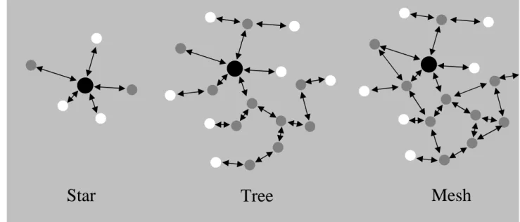
Driven by the need of simple network management and routing and the possibility of energy saving, three kinds of network topologies are widely used:

• Star, applied in home automation, PC peripherals, toys, games etc. It is merely used in small networks and is highly reliable on the center node. • Mesh, used in industrial control, wireless sensor networks and inventory tracking etc, where the network size is usually large. Compared with tree topology, mesh provides more reliability, which is an important reason of its popularity.

• Cluster Tree, in special case of Peer-to-Peer with many full function devices (FFD, described later).

Figure 2.2-Three kind of ZigBee network topologies

Addressing mode

Each node in a ZigBee network has two addresses, one is a 16-bit network address assigned when it joins the network. The other is a 64-bit extended address which is globally unique.

Device class and type

The devices are divided into two classes with different functionalities, so as to allow devices to have a simple design:

• Full function device (FFD) o Any topology

o PAN coordinator capable

o Communicate with any other device o Implements complete protocol set • Reduced function device (RFD)

o Limited to certain topologies o Cannot become a PAN coordinator

o Communicate only with a network coordinator o Very simple implementation

o Reduced protocol set

(14)

The devices are also classified to three types, according to the role they play in the network.

ZigBee Coordinator (ZC, the black ones in the center of figure 2.2, FFD)

Coordinator scans to find an unused channel to start a network. It is the first device in the network. The Coordinator node chooses a channel and a network identifier, also called PAN (personal area network) ID, and then starts the network. [5] Once the network is established, the ZC behaves like a Router node (or may even be removed). The continued operation of the network does not depend on the presence of the ZC due to the distributed nature of the ZigBee network.

ZigBee Router (ZR, the grey ones in figure 2.2, FFD)

Router scans to find an active channel to join, then permits other devices to join. It also assists in communication for its child end devices. In general, routers are expected to be active all the time and thus consume more power compared with end devices.

ZigBee End Device (ZED, the white ones in figure 2.2, FFD or RFD)

As the name implies, End Device is the “end” of the network. It does not support child devices and will always try to join an existing network. An end-device has no specific responsibility for maintaining the network infrastructure, which saves a lot of power and memory. Thus it can be a battery-powered node.

2.1.2 Operational mode

A ZigBee network can work in either beacon-enabled mode or non-beacon-enabled mode.

In beacon-enabled mode, the ZC and ZR transmit beacons periodically to confirm their presence to other network nodes, see [6]. Figure 2.3 shows the behavior of ZC and ZED.

• From ZC to ZED;

o ZC announces in the beacon of data pending

o If the data is destined to it, ZED sends a data request to ZC using slotted CSMA-CA (Carrier Sense Multiple Access with Collision Avoidance, described in appendix [A])

o After receiving the request, ZC sends an acknowledgement (ACK) back and then sends the data to ZED

o ZED acknowledges if it receives the data successfully • From ZED to ZC;

o ZED listens to beacon message and then gets synchronized with superframe structure

o After synchronization, it transmits data using slotted CSMA-CA o ZC acknowledges of data receiving (optional).

(15)

Figure 2.3-ZC and ZED behavior in Beacon Enabled Mode

In figure 2.3 and figure 2.4, ZC can be replaced by ZR. Actually, this behavior is between parent device and child device.

In non-beacon mode, the transmission from ZC to ZED is indirect, shown in figure 2.4.

• From ZC to ZED;

o Data is stored in ZC

o ZED polls ZC for stored data periodically using unslotted CSMA-CA (detail description in appendix [A])

o ZC acknowledges the poll and sends the data to ZED o ZED acknowledges of the data receiving

• From ZED to ZC;

o It simply transmits according to unslotted CSMA-CA

Coordinator to End Device

ZC ZED Data Request Acknowledgement Data Acknowledgement Beacon

End Device to Coordinator

ZC ZED

Acknowledgement Beacon

Data

(optional)

Beacon Enabled Mode

(16)

Figure 2.4-ZC and ZED behavior in Non-Beacon Enabled Mode In beacon mode, the ZC and ZR are also allowed to sleep in inactive period (mentioned later). The parents send beacon periodically to announce their existence, while child devices listen to the beacon and get synchronized. In this case, all the devices know when to communicate with each other. The most important advantage of beacon mode is that it reduces the power consumption of the system.

The drawback is devices cannot simply send out a beacon request to see whether there is a network to join. Instead, they have to listen and wait for a beacon, which obviously increases deployment time. Besides, precise timing is required. Devices that miss the beacon for some reason will lose the synchronization after a while. As a result, there is a broken link that will affect other nodes as well. Beacon mode is more suitable when the ZC is battery-operated, but it is not suitable for large networks, see [15].

Non-beacon mode is typically used for security systems where end devices units, such as intrusion sensors, motion detectors, and glass-break detectors, sleep most of the time. Power consumption is asymmetric in this mode, where ZC and ZR have to stay awake and is typically powered from main source. However, ZED is allowed to sleep for unlimited periods of time, enabling them to save power. This approach is widely used in large networks, see [19].

In the test, the system is operating in non-beacon enabled mode. Because packets are transmitted continuously, if ZC and ZR go to sleep, it would increase the test time.

Coordinator to End Device

ZC ZED

Data Request Acknowledgement

Data

Acknowledgement

End Device to Coordinator

ZC ZED

Acknowledgement Data

(optional)

(17)

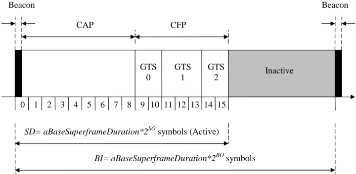
A superframe structure is used in beacon mode:

Figure 2.5- Superframe structure, each two superframes are separated by a beacon Each superframe consists of an active period followed by an inactive period. Two consecutive superframes are separated by a beacon.

Each active period consists of 16 equal-length slots and can further be partitioned into a contention access period (CAP) and a contention free period (CFP). Slotted CSMA/CA is used in CAP, devices have to contend for medium access. If a device requires fixed transmission rate, it can ask for guarantee time slots (GTSs). The maximum number of GTS in CFP is 7 and each GTS may occupy more than one slot. [2]

Two network configuration parameters are essential to determining the duty cycle of any device: the beacon order (BO) and the superframe order (SO). BO

determines how often the beacon is broadcasted (beacon interval); SO determines the active period duration within the superframe structure.

Formulas

• aBaseSlotDuration = 60symbols, which is 0.96ms since the symbol rate is

62.5ksymbols/s.

• aBaseSuperframeDuration = aBaseSlotDuration * 16 slots = 960symbols =

15.36ms

• Superframe Duration (SD) = aBaseSuperframeDuration*2SO symbols

(duration of the active part)

• Beacon Interval (BI) = aBaseSuperframeDuration*2BO symbols (duration of

the whole superframe)

In these formulas, 0<=SO<=BO<=14. BO=15 means it is operating in non-beacon mode and SO=BO means there is no inactive period, see [8].

0 1 2 3 4 5 6 7 8 9 10 11 12 13 14 15 GTS 1 GTS 2 GTS 0 CAP CFP Beacon Beacon

SD= aBaseSuperframeDuration*2SO symbols (Active)

BI= aBaseSuperframeDuration*2BO symbols

(18)

ZigBee standard also supports self-forming and self-healing, which makes the implementation and maintenance much easier. The association and disassociation functions are embedded in its MAC sublayer. When a network starts, ZC selects a channel and identifier (ID) for the PAN and assigns a 16-bit short address (network address) for a device. When a new device joins, it sends an associate request to get a network address. A device is considered orphaned if it misses aMaxLost-Beacons (default value is 4). The orphaning mechanism enables the network to detect link or node failure, thus to be self-healing, see [1].

2.1.3 ZigBee layer structure

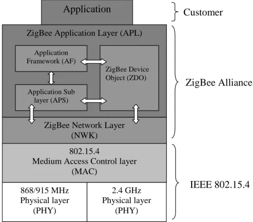
All ZigBee technology devices implement layered stack architecture. The ZigBee stack uses the IEEE 802.15.4 Physical (PHY) and Medium Access Control (MAC) Layers. In addition to the IEEE layers, the ZigBee Alliance has defined a set of standardized layers that sit on top of the IEEE layers and together these layers make up the ZigBee technology stack architecture.

Figure 2.6-ZigBee four-layer structure

The lower layers (including PHY/MAC, Network and Security layers) make up the ZigBee stack. The application layer can be further divided into three layers: ZigBee Device Object layer, Application Framework layer and Application Sub layer.

(Detailed description is given in appendix [D].)

Customers can build up their own applications in application layer. In the tests performed, an application is implemented in the application layer to measure the packet round trip time (RTT).

ZigBee Alliance 868/915 MHz Physical layer (PHY) 2.4 GHz Physical layer (PHY) 802.15.4

Medium Access Control layer (MAC)

ZigBee Network Layer (NWK)

ZigBee Application Layer (APL)

IEEE 802.15.4

Application

_Customer

Application Framework (AF) Application Sub layer (APS) ZigBee Device Object (ZDO)

(19)

2.1.4 ZigBee frame structure

Figure 2.7 shows the structure of a ZigBee frame and also the content of header and footer. When sending a packet, it is first generated in the application layer and then added with network header, MAC header and physical header.

Figure 2.7-ZigBee Frame structure (See the full name of the abbreviations in appendix [B].)

The maximum payload size supported by the application layer is based on the settings of lower layers. The ZigBee standard has declared that the maximum PHY packet size is 127bytes. The actual data rate is dependent on the protocol overhead added. A variety of headers from 9 to 25 bytes can be added to the payload,

depending on addressing field and security header. Ultimately, the user doesn’t have to know all the settings in order to get the maximum payload size, or

maximum transport unit (MTU). A function to query MTU is provided by AF layer, see [5].

2.1.5 Comparison with Wi-Fi and Bluetooth

The term Wi-Fi is often used as a synonym for wireless local area network (WLAN). It is mostly used for data transmission, with a long range and a data throughput of 2-11Mbps.

ZigBee and Bluetooth have much in common. Both are types of IEEE 802.15 "wireless personal-area networks," or WPANs. They both run in the 2.4-GHz unlicensed frequency band, and use small form factors and low power.

However, ZigBee is focused on control and automation, exchanging small packets over large network; while Bluetooth is focused on connectivity between laptops and PDA’s, as well as more general cable replacement. Compared with ZigBee network, large packets are transmitted over small network. A comparison of these three technologies is also shown in figure 2.8 and table 2.2.

PHY Layer MAC Layer Preamble Sequence Start of Frame Delimiter Payload Address Information Data Payload FCS Auxiliary Security Header Data Sequence Number Frame Control Frame Length

PHY Protocol Data Unit (PPDU)

MAC Protocol Data Unit (MPDU)

MHR MSDU MFR PSDU SHR PHR Octets: 2 1 4 to 20 n 2 0,5,6,10 or 14

(20)

Range P e a k D a ta R a te Smaller Larger S lo w e r F a s te r 802.11g 802.11b 802.11a Bluetooth™ ZigBee™ Wi-Fi®

Figure 2.8-Range and Data Rate comparison of ZigBee, Bluetooth and Wi-Fi, see [3] The following table also shows a comparison of these wireless standards:

ZigBee 802.15.4 Bluetooth

802.15.1

Wi-Fi 802.11b

Applications Monitoring and control

Cable replacement Web, video, email

Data capacity 250Kbps 1Mbps 11Mbps

Range (meters) 75 (typically) 10-100 100

Battery life years days hours

Nodes per network up to 65,533 8 30

Software size (Kbytes)

4 - 32 250 >1,000

Table 2.2-General comparison of ZigBee, Bluetooth and Wi-Fi, see [3]

2.2 Introduction to Z-Stack Development Kit

Z-Stack is Texas Instrument’s (TI) implementation of the ZigBee specification. As mentioned earlier, the lower layers (including PHY/MAC, Network and Security

layers) make up the ZigBee stack. A user application can be built upon the Z-Stack. In this thesis work, CC2430 (Chipcon products from Texas Instrument) Z-Stack Development Kit (CC2430ZDK) is used to develop user application. The CC2430ZDK is designed to deliver elements for ZigBee development. It is a very flexible kit that

(21)

can be used to develop everything from simple light switches to advanced nodes with lots of peripherals.

A complete development kit includes: • TI's ZigBee stack, Z-Stack

• 2 SmartRF04EB Evaluation Boards (Figure 2.9) • 2 CC2430EM Evaluation Modules (Figure 2.9) • 5 CC2430DB Demonstration Boards (Figure 2.10) • Antennas and batteries

• IAR EW8051 C-compiler with C-SPY debugger • Sensor Network Analyzer from Daintree

Figure 2.9-Chipcon SmartRF04EB Evaluation Board with CC2430EM. The antenna is Titanis antenna from antenova® _{(a picture from TI)}

(22)

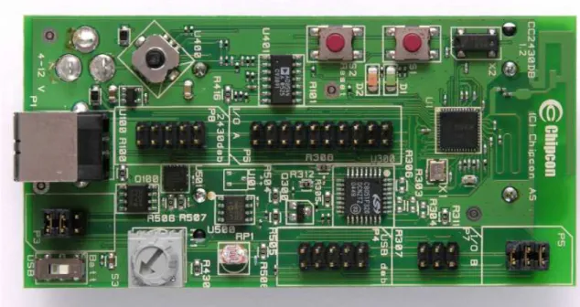
Figure 2.10-Chipcon CC2430DB Development Board (a picture from TI) The hardware included in the kit contains necessary support to evaluate,

demonstrate, prototype and develop software targeting various ZigBee applications. The SmartRF04EB provides the user with functionality such as joystick, buttons, USB port, RS-232 port and an LCD display. This board also includes hardware support for programming CC2430EMs and custom made boards.

The CC2430DB demonstration board will render it possible to implement true low power applications that can last on batteries for years. CC2430EM uses Titanis antenna, providing a better performance than that in CC2430DB, which is embedded in the Printed Circuit Board (PCB). A joystick on C2430DB or on

SmartRF04EB provides five switches as input. The five switches are triggered when joystick is pressed against a position or pressed down.

Press down SW5 Left position SW4 Down position SW3 Right position SW2 U400 position SW1 Joystick Switch Press down SW5 Left position SW4 Down position SW3 Right position SW2 U400 position SW1 Joystick Switch

(23)

Sensor Network Analyzer (SNA) from Daintree is a well known expert tool for ZigBee, which not only allows the user to view the network as a whole, but also to look into the content of an individual packet. The 2400E Sensor Network Adapter acts as an observation and control point enabling the use of SNA in live wireless sensor networks. The adaptor can also be replaced by a sensor board (CC2430DB or smartRF04EB with CC2430EM).

(24)

Chapter 3 3. Packet Delay and Range Study

3.1 Test implementations and preparations

3.1.1 Round trip time (RTT) calculation

An application built on Z-stack is implemented to measure the round trip time (RTT) from coordinator to a specific device in the network.

Figure 3.1-A round trip of a packet

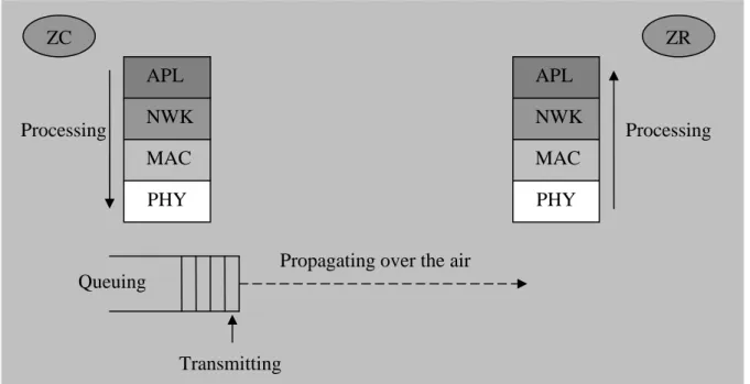
RTT is calculated in the application layer. Here the acknowledgement (ACK) is sent and processed by MAC layer so the application layer won’t be aware of it. In this case, the RTT is calculated from sending the message to receiving the reply. The entire process of packet transmission is shown in the figure below.

Figure 3.2-Packet transmission process from ZC to ZR (one way) Processing APL NWK MAC PHY Queuing Transmitting

Propagating over the air

APL NWK MAC PHY Processing ZC ZR ZC ZR/ZED Send a message ACK

Send the reply RTT

(25)

According to Figure 3.1 and Figure 3.2, RTT is calculated from when a packet is generated in APL and send to lower layers, to the time APL receives the response from the target device. It consists of four parts:

• Processing time, add or remove headers;

• Queuing time, in indirect transmission, packet will be held in the parent before its child polls. It also includes the time for the node to gain medium access;

• Transmission time, at a transmit speed (250kbps); • Propagation time, propagating over the air.

If a packet is lost during the transmission, retransmissions will also contribute to the whole RTT.

Retransmission is dealt by the APS layer, the NWK layer and also the MAC layer. If APS acknowledgement is enabled, APS layer will attempts several times

(configurable, default value 3) before receiving ACK. The NWK layer also performs a number of retries (configurable, default value 2) for the next hop message, once the MAC layer retries are exhausted for that message. MAC-level

acknowledgements and retries are default and automatic regardless of service used, see [23]. MAC layer will retry 3 times (configurable) before returning a failure

status to the network layer. The time interval between each attempt depends on the CSMA/CA algorithm.

Here in the test, APS layer acknowledgement is disabled thus APS layer will not retransmit; NWK layer performs 2 attempts for the next hop message, the interval is unpredictable, depending on the packet length, surroundings and distance

between nodes; MAC layer will retry 3 times for each attempt before announcing failure, and delays a random amount of time (from 3ms to 10ms) before each attempt. In the worse case, the sender will transmit at most 8 times and the

receiver will attempt 8 times to respond as well. According to the packets captured by SNA in the case of retransmissions, the timeout timer is set to 1s for ZR and 3s for ZED (dependent on POLL_RATE, in the test, poll rate for ZED is set to 1000ms).

3.1.2 Implementation

Input keys designed: (switch settings shown in figure 2.11)

• Press SW3 (only valid in ZC): start a new measurement by generating a prompt.

• Press SW4: generate a group broadcast (multicast) message.

In the application, the measurement starts by generating a group broadcast

(multicast) message from the ZC. When ZR or ZED receives the message from ZC, it replies with its unique 64-bit extended address; the devices are then numbered as index according to the order of receiving their responses. ZC records the index, network address and extended address of the devices in a table.

New devices can also join the network by sending a group broadcast message. When ZC receives the multicast message from a device, it checks if the device is already in the network. If yes, it prints out the index and the role of the device (ZR or ZED). Otherwise it adds the new joined device into the network.

A prompt window is used to set a series of parameters by the user: • Target device for the test (sweep all is also supported)

(26)

• Payload length

• Interval between packets • Number of packets to transmit • Number of rounds to repeat the test • Interval between rounds

The application uses UART (Universal Asynchronous Receiver Transmitter, used for serial communications over a computer or peripheral device serial port) to

communicate with the computer. It reads the settings from the computer and starts the test. Packets are generated based on the settings and transmitted with a

window size of one, which means that the sender will not send a second packet until it receives the ACK from the receiver. A timeout timer is set for every packet. If the sender receives the ACK before timeout timer is fired, the total round trip time is calculated according to system clock (accuracy 1ms) and printed in the

computer through UART. If not, a packet is considered lost and “timeout” is printed. The result is then processed by Matlab to check the transmission condition,

including packet loss rate and average RTT. Some figures are also plotted for analysis.

Only one set of code is implemented and different functions are implemented according to the role of the device, whether it is ZC, ZR or ZED. There are also some other features that can be added. Security can be enabled to ensure message integrity; power saving can be enabled to allow device to sleep and save energy.

After the settings, the measurement starts and Sensor Network Analyzer (SNA) also begins to capture the traffic in the network to monitor the entire process of the test. The received power of the packet is also recorded by SNA.

Figure 3.3-General test scenario

Actually the received power recorded is not the received power of the device performing the test (ZC). Only one program can be running on CC2430EM, either the test application or SNA that captures the traffic. When performing the tests, two smartRF04EB evaluation boards with CC2430EM are placed next to each other. One of them is running the test application and the other one is running SNA. Since

ZC Target Device

Device running SNA

(27)

the two boards are exactly the same, it can be assumed that the received signal strength at the two boards is quite close. As the one used for capturing packet only listens to the network, they don’t interfere with each other.

The test bench can be used as a simulation tool to evaluate the transmission condition when installing the meters.

3.1.3 Radio transmission range factors

Radio waves propagate in a straight line in several directions at once. In a vacuum, radio waves propagate at 3*108_{m/s. The signal gets weaker due to}

• Reflection • Refraction • Diffraction • Absorption

In the air, the signal strength attenuates as it travels through the medium because of these reasons; the received signal strength decreases when the distance

increases. However, it is not decreasing linearly since the environment diversifies and is frequently changing.

There are many factors that would affect radio transmission:

Transmit power

The transmission power is the key determinant of transmission range. The output power of CC2430 radio is programmable, from 0.6dBm to -25.2dBm.

Receiver sensitivity

Higher receiver sensitivity leads to a larger range. In order to be received correctly, the signal strength of a received packet has to be larger than receiver sensitivity. With packet error rate (PER) smaller that 1%, the receiver sensitivity is -85dBm at 2.5GHz band and -92dBm at 868/915 MHz band.

Antenna design

The type of antenna and the height of antenna also affect transmission range. In order to exclude the undesired influence of this factor, the antenna is fixed to a height of 1.5m in all the tests performed.

(28)

Figure 3.4- Fresnel Zone

This figure shows the line-of-sight condition. Radio is transmitted in a zone, instead of a direct line between the two antennas. The transmission zone is known as a Fresnel Zone, which is a three dimensional ellipsoid with the two antennas at the foci of the ellipse (Huygens–Fresnel principle). The more of the Fresnel Zone that is free from obstructions, the better the transmission will be.

If both antennas can be lifted so that there are no obstructions inside of the Fresnel Zone, the radio transmission will be improved. This consideration is particularly important if one of the antennas is to be mounted close to the ground. That positioning, in effect, eliminates about one half of the Fresnel Zone and reduces range dramatically.

Reflection surface

The reflecting surfaces do not need to be on a direct reflective path. Radio waves do not bounce off of reflective surfaces like pool balls bounce off the rail of the pool table. Each radio wave initiates a new omni-directional spherical wave at each reflective surface that it encounters, according to Huygens-Fresnel principle. A type of chaotic pattern ensues that allows some of the transmitted radio energy to reach its final destination by reflected signals. A flat water surface is also a good radio wave reflector for this type of radio transmission.

Absorption surface

Absorption surfaces have the opposite effect of reflecting surfaces. These surfaces stop the radio energy from its path. Earth and concrete are very effective in

absorbing radio wave energy. Grass and trees absorb to a less extent, but are known to be good absorbers of radio energy.

These absorption surfaces can have a dramatic effect on the radio transmission distance.

Acceptable packet loss rate

The maximum transmission range also depends on the acceptable packet loss rate by the users. As mentioned earlier, signal strength decreases with distance. With weaker received signal, packet loss rate will be higher.

Transmitting Antenna

Receiving Antenna Direct Radio Path

(29)

Humidity

Humidity is also a factor that affects radio transmission. High humidity would decrease the performance of radio transmission dramatically.

In order to avoid the undesirable influence of some factors, some parameters are fixed in all the tests:

• Humidity is recorded in the tests;

• WLAN exists in all the indoor tests (widely used in most buildings); • Transmit power is fixed to -1.5dBm;

• The antennas of both sender and receiver are fixed to a height of 1.5m because in reality the meters are normally mounted on the wall;

• ZC is the source and ZR is picked as the destination, not a ZED, since the RTT of ZED simply adds the sleep time and thus to increase time of test.

3.2 Tests and result analysis

The test scenarios are designed according to the installation cases of electricity meters. The communication of two devices may happen in the open air within line of sight, in a corridor with line of sight, or indoor with some obstacles in between. Note that all the devices are fixed to a height of 1.5m in all tests because the electricity meters are usually mounted against the wall with a certain height. Also note that the results may vary by a small amount when the test is repeated. Because the environment is frequently changing and the number of samples is limited in the test. Not every result is analyzed here in this report but only the typical experimental results. Some other test results are attached in appendix [F]. 3.2.1 Outdoor test

Test conditions:

• Environment: In a typical parking lot; • Temperature: 8-10˚C;

• Humidity: 75.5%;

• Weather: Sunny and cloudy;

• Battery voltage: 3.12V. (Note that CC2430 can work in a wide range of voltage, from 2.0V to 3.6V. It will work properly if the supply voltage is in this range.)

Test settings:

• Target device for the test: Router 0 (point to point communication) • Payload length: 50bytes (MTU supported is 85bytes)

• Interval between packets: 100ms • Number of packets to transmit: 100 • Number of rounds to repeat the test: 20 • Interval between rounds: 1000ms

• Output power: -1.5dBm • Security: Disabled

• APS acknowledgement: Disabled

2000 samples are collected in the test. In the result obtained, most of the RTT falls below 100ms and quite few RTTs are larger than that. In order to show the

distribution more clearly, only the parts falling below 100ms are shown in the scattergrams.

(30)

Scenario 1

In open path (line of sight), perform measurements with a distance from ZC to ZR of 5m, 10m, 20m, 40m, 50m, 75m and 85m until the maximum range is found (with packet loss rate of 1%). The received power and RTT are recorded;

Figure 3.5-Scenario 1, a single hop with a distance from 5m to 85m (a photo of the test scenario is attached in appendix [E])

Result and analysis

Let’s first have a look at the scattergrams of RTT for 20m, 50m, 75m and 85m and compare the packet loss rate.

Figure 3.6-Scattergram of RTT with distances from 20m to 85m (The part in the rectangle is zoomed in and shown in the following figure.)

ZC ZR

(31)

Figure 3.7-Zoom in version of scattergram of RTT for 20m in Figure 3.6 (As the accuracy of system clock is 1ms, the RTT obtained is always an integer value.)

Distance Average RTT Packet loss rate Concentration

20m 18.0ms 0% 100%

50m 17.9ms 0% 99.95%

75m 17.9ms 0.75% 97.95%

85m 18.6ms 1.65% 95.95%

Table 3.1-Comparison of transmission condition with a distance from 20m to 85m (Concentration means percentage of RTT between average ± 5ms)

The received signal strength is also recorded by SNA when performing the tests. The following table shows the average received power of the packets with different distances. It is calculated by the average of 20 samples picked randomly from all the 2000 samples.

Distance 10m 30m 50m 75m 85m

Received power -66dBm -73dBm -78dBm -84dBm -86dBm Table 3.2-Received power with a distance from 10m to 85m

As mentioned earlier, signals attenuate along the way of propagation. With weaker received signal strength, the probability of retransmissions gets higher. In this case, RTT gets higher and packet has a larger chance to be lost in the transmission. We can see from table 3.1 that packet loss rate does increase with longer distance. When packet loss rate is relatively low, and the probability of retransmission is also low, the average RTT doesn’t change much with the increase of distance (from 20m to 75m in table 3.1). The reason is that, for the four parts of RTT (mentioned

(32)

previously), only propagation time changes when distance changes. However, radio waves are propagating at the speed of light, at 3*108 _{m/s. When distance rises}

from 5m to 75m, the propagation time only changes by around 0.2µs. So the influence of distance is small enough to be neglected.

It is also noticeable that there is a small decrease of RTT from 20m to 50m, which results from limited number of samples. It would be more accurate if more samples are collected.

From 75m to 85m, when signal strength gets weak, retransmission happens more often. As a result, the RTTs distribute more diversely, the average RTT raises considerably and packet loss rate increases as well.

With a packet loss rate of 1%, it can be concluded that the maximum range of a single hop is between 75m and 85m.

Let’s look further at the histogram and accumulative curve of RTT with different distances and see how RTT is distributed.

Figure 3.8-Histogram of RTT with a distance of 20m, 50m and 75m (RTT>35ms is rounded to 35ms)

In this figure, the RTT for all the three charts are highly centralized around 18ms. Almost all the RTTs fall between 14ms to 21ms. There’s little difference among the three bar charts, except that the one for 75m has a small portion of RTT that is above 35ms. That part includes both longer RTTs and packet losses (RTT=infinity).

(33)

Figure 3.9-Accumulative curve of RTT for 50m, 75m and 85m

Figure 3.10-Zoomed in accumulative curve of RTT for 50m, 75m and 85m The two accumulative curves clearly show that RTT is more diversely distributed with a longer distance. The dash lines present that 95%, 97.5% and 99% of the RTT fall below 20ms with a distance of 85m, 75m and 50m.

Scenario 2

Two tests are performed with 2 hops and 3 hops between ZC and ZR, each one with a distance of 50m.

(34)

Figure 3.11- Scenario 2 test with 1 hop, 2 hops and 3 hops

Result and analysis

A router in between is acting like a repeater. It reconstructs the packet and forwards it to the destination, thus regenerates the radio signal.

However in the mean time, routers have to process the received packets before forwarding them. This will add more processing time thus lead to a larger RTT. It is also learned from table 3.3 and the figure 3.12, RTT rises considerably with the increasing of number of hops. Distance is not a factor that would contribute much to the whole RTT, as mentioned before.

Table 3.3 shows the change of RTT when hop number varies.

Hop Number 1 hop 2 hops 3 hops

Average RTT 17.9ms 32.9ms 48.2ms

Table 3.3-Round trip time with 1 hop, 2 hops and 3 hops

ZC ZR ZR ZR

50m 50m 50m

(35)

Figure 3.12-Round trip time with 1 hop, 2 hops and 3 hops

Scenario 3

In scenario 2, it was found that the maximum range of the second hop is a little smaller than the first hop. The difference between them is that ZC has a better antenna than that of ZR (CC2430EM has a better antenna than CC2430DB). That might be the reason of the longer range. Another set of test is performed to see the influence of a better antenna.

Two tests are performed with a distance of 85m, one with CC2430EM on both sides and one with CC2430EM on only one side.

Figure 3.13-Scenario 3 test with different antennas

ZC ZR (CC2430DB) 85m ZC ZR (CC2430EM) 85m Test 1 Test 2

(36)

Result and analysis

The antenna does influence the test results. It is obviously shown in figure 3.14 that the transmission condition becomes better with a Titanis antenna. Average RTT becomes lower, packet loss rate is very low and it is highly concentrated as well. Due to the limited number of samples and frequently changing environment, the result for 85m in this scenario is different from that in scenario 1 (table 3.1).

Figure 3.14-Embedded PCB antenna Vs Titanis antenna 3.2.2 Indoor test

Test conditions:

• Environment: ABB Corporate Research office building (206) • Temperature: 21˚C;

• Humidity: 50%;

• Battery voltage: 3.02V. (within supply voltage)

Test settings:

• Target device for the test: Router 0 (point to point communication) • Payload length: 50bytes

Titanis antenna Embedded PCB antenna

(37)

Scenario 1

A series of tests are performed in the corridor within line of sight, with a distance from 10m to the maximum range and compare the result with outdoor test. (Here the test is done on floor C, the third floor. A floor plan is attached in appendix [E].)

Result and analysis

Distance Average RTT Packet loss rate

Concentration Received power

20m 18.0ms 0% 98.7% -68dBm 50m 18.1ms 0% 99.7% -70dBm 70m 18.4ms 0.1% 94.8% -75dBm 90m 18.9ms 0.05% 93.6% -78dBm 105m 18.0ms 0.05% 97.05% -81dBm 115m 18.2ms 0.1% 96.5% -82dBm

Table 3.4-Comparison of transmission condition with a distance from 20m to 115m in the corridor of floor C

Compared with the results from outdoor test,

• The maximum range is much longer, more than 115m (as the total length of the corridor is around 120m, it’s not possible to get the maximum range) • The signal attenuates slowly since the reflection from the wall strengthened

the signal. The tradeoff is that the received power is not as stable as in outdoor line of sight.

• The influence of distance on RTT is also neglectable when the packet loss rate is low.

Scenario 2

As the floor plan is unique, it may be meaningful to repeat the same test in different floors and compare the result. The floor plan of floor A and B is also attached in appendix [E].

Note that from this test, the smartRF04EB with CC2430EM for SNA is replaced by 2400E Sensor Network Adapter due to equipment issues. In this case, the received signal power is not the same as that in ZC. But it can still be used for performance evaluation since only the reference device is changed.

Result and analysis

Similarly, signal strength attenuates very slowly along with distance in general trend. The maximum transmission range is also very close in different floors. As the structure of the corridor is not symmetric and changes frequently along the way, which affects the reflection, the signal strength is not decreasing linearly with longer distance. Concentration is fluctuating as well, shown in table 3.5.

In addition, due to the variation of floor plan and furniture placement, received signal strength also varies in different floors.

(38)

Floor (A is first floor)

Distance Average RTT Packet loss rate Concentration Received power 50m 17.4ms 0% 97.55% -78dBm 70m 17.9ms 0% 96.35% -72dBm 90m 18.3ms 0% 97.75% -82dBm A 100m 17.7ms 0% 97.45% -84dBm 50m 17.7ms 0% 98.45% -65dBm 70m 18.1ms 0% 98.75% -65dBm 90m 17.3ms 0% 99.15% -67dBm B 100m 17.8ms 0% 98.1% -74dBm 50m 17.9ms 0% 95.75% -75dBm 70m 18.4ms 0.05% 94.9% -76dBm 90m 18.0ms 0% 97.35% -78dBm C 100m 17.3ms 0% 98.5% -75dBm

Table 3.5-Test result comparison in floor A, B and C (Note that the test in floor C is done a second time, so the result is different from that shown in table 3.4.)

Scenario 3

Several tests are performed with different doors in between and in different floors and the results are compared to see how the transmission condition is affected by different obstacles.

A-Test with different doors between ZC and ZR (the distance between them is 10m)

ZC ZR

Glass door/ Iron door

(39)

B-Test in different floors (Note that the height of one floor is around 3m, so the distance between the two devices is around 4.5m, which is shorter compared with

the test in A)

Figure 3.15-Performance comparison with different obstacles between ZC and ZR

Result and analysis

Obstacle Distance Average RTT Packet loss rate Concentration Received power In line of sight 10m 18.2ms 0% 99.1% -69dBm 1 glass door (around 0.3cm thick) 10m 18.1ms 0% 99.8% -75dBm 2 glass doors 10m 18.3ms 0% 100% -78dBm 1 iron door (5cm) 10m 18.4ms 0% 100% -79dBm 2 iron doors 10m 23.7ms 3.55% 48.7% -86dBm 1 concrete floor (17cm) 3m 17.5ms 0% 97.75% -60dBm 2 concrete floors 6m 17.1ms 0% 96.95% -85dBm Table 3.6-Performance comparison with different obstacles in between (ZR loses connection with ZC when there are 3 concrete floors in between.)

Iron door has the most influence on signal attenuation, followed by concrete floors and then glass doors. The permittivity of different materials on radio propagation is studied in [24], which also shows that concrete blocks signal the most, and then glass and wood (iron is not given).

Scenario 4

A similar set of tests are performed in a living environment and see the difference from the result in office building. A sketch of floor plan in Skalden 2 apartment is shown in appendix [E].

ZC

Floor C corridor

ZR

(40)

Result and analysis

The following table shows a comparison of performance when the test is done in opposite room, respectively in line of sight, with one wood door in between and two wood doors in the way.

Obstacle Average RTT

Packet loss rate

Concentration Received power In line of sight 18.1ms 0% 98.7% Around -70dBm 1 wood door (6cm) 17.7ms 0.05% 97.8% Around -70dBm 2 wood doors 17.9ms 0.05% 96.85% Around -70dBm Table 3.7-Test the influence of wood doors (“around” means that the value is instable and fluctuating all the time)

As is obviously shown in the table, received signal strength remains the same when wood doors are in the way. The transmission condition also remains fairly good, which means that the blockage of wood doors is almost neglectable.

Office buildings are usually very tall, where security and stability is considered a big issue; concrete walls and floors, iron or glass doors are widely used. These are great reflectors of radio energy at 2.4GHz frequency band. While the residential buildings are considered “less iron”, where comfort is of vital importance; wood

doors and floors, and walls made from brick, stone or even wood are more common. Some other tests are also performed when nodes are placed in different spots. The result is attached in appendix [F].

3.2.3 Interference test

Test conditions:

• Environment: Apartment Skalden 2 • Temperature: 22˚C;

• Humidity: 55%;

• Battery voltage: 2.89V. (within the supply voltage range)

Test settings:

• Target device for the test: Router 0 (point to point communication) • Payload length: 50bytes

Scenario description

Interference is almost “inevitable”; there is no interference-free environment. Tests are performed to see how ZigBee reacts to interference from microwave oven, Bluetooth and WLAN, since they are all using the 2.4GHz frequency band.

(41)

Figure 3.16-Test scenario with microwave interference

Figure 3.17-Test scenario with Bluetooth interference (Two cell phones are transmitting data with Bluetooth)

Result and analysis

Table 3.8 shows that Bluetooth and microwave has a little influence on ZigBee network performance. Microwave oven, Bluetooth and WLAN are using the same frequency band with ZigBee, so the chance of collision gets higher when there is interference from either one of them. Correspondingly, it would increase the time to gain medium access and thus may lead to a longer packet delay (RTT) or even cause transmission timeout and packet discard. However, we can also see that the influence is very small, indicating that ZigBee is robust against interference.

Scenario Average RTT Packet loss rate Concentration Received power Corridor without interference 16.6ms 0% 99.05% -62dBm Corridor with Microwave interference 19.2ms 0.15% 89.95% Around -69dBm Opposite room without

interference 18.1ms 0% 98.7%

Around -70dBm Opposite room with

Bluetooth interference 18.2ms 0.1% 97.4%

Around -67dBm Table 3.8-Influence of interference on packet transmission

ZC ZR

Floor C corridor

Sony Ericsson C902

Sony Ericsson K530i

ZC ZR

Floor C corridor Microwave oven

(42)

Chapter 4 4. Other Performance Metrics

4.1 Power Consumption Measurement

Power management is used by battery powered ZEDs to minimize the power consumption between brief periods, either during scheduled activity or during a long time sleep. System activity is monitored after each task finishes its processing. The system will decide whether to sleep or not according to the monitoring, see [20].

A power consumption test was performed according to [21] A standalone

CC2430EM is used in the measurement to exclude the extra power consumption by the board, thus it would be closer to the theoretical result. The circuit is connected as follows:

Figure 4.1-Power consumption measurement circuit (The Oscilloscope measures the voltage on the resistor and the current can be calculated by dividing the voltage

read from Oscilloscope by 10Ω.)

In the power consumption test, several scenarios that can occur to electricity

meters in reality life are designed and the power consumption of them is measured. The test application is implemented in both ZC and ZED. Also note that security is not enabled in all the tests performed.

4.1.1 Polling without data transmission

ZED sends poll to ZC every 500ms for data pending. The size of the polling packet is 12bytes (verified by SNA).

Oscilloscope Resistor 10Ω Power supply (3V) _─ + SmartRF04EB with CC2430EM (ZC) CC2430EM (ZED) Amplifier

(43)

Result and analysis

Figure 4.2 shows the current consumption when ZED polls ZC every 500ms, but there is no data stored in ZC for ZED. The current is calculated by dividing the voltage by 10Ω.

Figure 4.2-Polling without data transmission (The two parts in the rectangle are zoomed in and shown in figure 4.3 and 4.4. Note that the scale of x-axis is 200ms, and for y-axis it is 50mv, which are marked by the two ellipses in the figure. In this case, the current of one grid is 50mv/10Ω=5mA. The scales of the following figures

are shown in the same place.)

Figure 4.3-Zoomed in of part 1 in Figure 4.2 (It shows a full sequence of ZED from waking up and starting to transmit, to shutting down and going to sleep again. The scale of x-axis is 1ms and for y-axis it is 50mv. It is shown in the same place as in figure 4.2 and so it is with the following figures.)

500ms 1 2 1 2 3 4 5 6 7 8 9

(44)

ZED consumes different amount of power at different stages. The following table shows a detailed description of the events at each stage and the current and

duration as well. The scale of x-axis in this figure is 1ms and that of y-axis is 50mv, correspondingly 5mA per grid. Note that the power consumption is shown in the form of charge so that the battery life can be calculated according to the data transmitted each day.

Stage Description Current (mA)

Duration (ms)

Charge (mA*ms) 1 Start up sequence. MCU in active

mode running on 16 MHz clock

7.5 0.5 3.75

2 MCU running on 32 MHz clock 12 1.6 19.2 3 CSMA/CA algorithm. Radio in RX

mode. 31 1.5 46.5

4 Switch from RX to TX. 17.5 0.2 3.5 5 Packet transmission. Radio in TX

mode.

29.5 0.6 17.7 6 Switch from TX to RX. 18 0.1 1.8 7 Reception of acknowledgement

from ZC. Radio in RX mode.

31 1.1 34.1

8 Packet processing. MCU running on 32 MHz clock.

12 1.1 13.2

9 Shut down sequence. MCU running on 16MHz.

7 0.6 4.2

Table 4.1-Description and power consumption of each stage (according to [21]) The total duration of one active period is 7.3ms and the total charge is

143.95mA*ms, according to figure 4.3 and table 4.1. At stage 5, ZED is

transmitting the polling packet at a certain data rate. The duration of this stage is dependent on the packet length. In this case, the charge of transmitting 1 byte is 17.7/12=1.475mA*ms.

The maximum current in the whole sequence is around 31mA, when the device is in RX mode. After the polling, ZED goes to sleep again, and the current consumption is shown in the zoomed in figure below:

Figure 4.4-Zoomed in of part 2 in Figure 4.2 (It shows the current consumption when the devices enters sleep mode.)

(45)

There are two sleep modes provided by Z-Stack, LITE sleep and DEEP sleep. LITE sleep is used when the device needs to wake up and perform a scheduled activity (such as polling). DEEP sleep is used when there’s no scheduled activity for the device. If the device needs to wake up, an external stimulus is required, such as a button press. Here in the test, LITE sleep mode is used since the ZED is polling periodically. When it enters LITE sleep mode, the average current consumption is less than 20µA. The value is even less in DEEP sleep mode.

4.1.2 Polling with data transmission

In this scenario, ZED is polling ZC every 500ms for the data pending with a packet size of 12bytes as well. ZC sends packets periodically to ZED, one at a time with a size of 50bytes. (It won’t send a second packet until receiving the

acknowledgement from ZED.) When ZED receives a packet from ZC, it sends an acknowledgement back.

Result and analysis

The following two figures show the whole process of transmission of ZED.

Figure 4.5-Polling with data transmission (The part is in the rectangle is also zoomed in and shown in the following figure.)

In part 1 of figure 4.6, ZED starts up, polls the ZC, and receives the data stored for it and then goes to sleep again. A detailed events description is outlined in [21]. In part 2, after receiving the packet from ZC, ZED sends a response message back. There are fewer stages compared to part 1 since ZED simply checks the medium and transmits the message.

(46)

Figure 4.6-Zoomed in version of Figure 4.5 4.1.3 Join and rejoin process

In a running network, it’s not uncommon for a device to lose association with its parent. When this happens, it always tries to rejoin the network by generating beacon request periodically. When a device tries to join a network, it will broadcast beacon request periodically until it finds an available network. This process might as well consume a considerable amount of power. Hence it is also meaningful to study the energy consumption of join process. In this scenario, ZC is first shut down and ZED is restarted to see the joining process of an end device.

Result and analysis

Figure 4.7 shows the power consumption of the join process. The interval between each attempt is random and configurable.

Figure 4.7-Power consumption of join process (In one cycle, the active period duration is 500ms)

1 2

(47)

The following figure shows the rejoin process when ZED losses connection with ZC. When the device loses connection to the ZC, it will try periodically to rejoin the network, with a random interval depending on the configuration.

The rejoin process should go faster as the device already knows which network it wants to rejoin, while in a join process it first has to do the scan for an available network and then start the process. The active period duration of both join and rejoin process can be lowered by reducing the scan duration in the application.

Figure 4.8-Power consumption of rejoin process (In one cycle, the active period duration is 80ms)

4.2 Throughput

As mentioned in chapter 2, ZigBee supports a maximum over-the-air data rate of 250kbps for the 2.4GHz band. However, in reality, the effective data rate is somewhat lower because of the protocol overhead. The theoretical value of effective data rate is calculated in detail in [13] by Jennic Ltd.

In throughput test, a sample application is implemented in one ZC and one ZR to measure the actual data rate. In this test, the sender transmits immediately when it receives AF_DATA_CONFIRM_CMD, which is received as a confirmation of a data packet sent. When the receiver gets a packet from the sender, it checks if the size and the content of the packet are correct or not. If not, the packet is discarded and not calculated in received bytes.

The following two figures show the result measured by SNA, note that

1) “Stream Summary: 0000:0001” means that PAN ID is 0000 and source node’s network address is 0001.

2) “APS Tx Cum” is the maximum transmit rate occurred, while “APS Tx Inst” Means the instant transmit rate.

(48)

Figure 4.9-Maximum data rate in one way transmission (from ZC to ZR, without collision)

Figure 4.10-Maximum data rate in two-way transmission (both ZC and ZR are transmitting, with collision)

According to figure 4.9 and 4.10, the effective data rate is 95kbps if only ZC is transmitting. When the two devices are both transmitting and receiving, the

effective data rate per node decreases to around 47kbps because of the collisions in the network. However the total throughput of the network is almost the same

(around 95kbps), which is about two fifths of the theoretical data rate.

4.3 Network Size and Addressing

The number of nodes in a ZigBee network can go up to 65533. A 16-bit network address, which means a total of 65536 addresses, is assigned to a device when it joins. However, 0xFFFF is a broadcast address for all the devices in the network; 0xFFFD is a broadcast address for the devices that are not sleeping while 0xFFFC is used to send a message to all routers. [5]

(49)

• MAX_DEPTH (Lm) parameter determines the maximum depth of the network. The ZC is in depth 0 and its child is in depth 1 and so on.

• MAX_CHILDREN (Cm) determines the maximum number of child nodes that a router can possess.

• MAX_ROUTERS (Rm) determines the maximum number of router-capable child node that a node can possess.

The network address is assigned according to Cskip algorithm, which is also

dependent on the three parameters, see [14] The Cskip value of device in a certain depth is determined by a formula (There is a slight difference for ZED with Cskip>0, see the detailed information in [14]):

Formula 4.1-Cskip algorithm

The parent will assign the network addresses to its children with an interval of Cskip. For example, in the test application, Lm=5, Cm=20 and Rm=6. According to the formula,

Depth 0 1 2 3 4 5

Cskip 5181 861 141 21 1 0

Table 4.2-Cskip algorithm example (With a Cskip of 0, the node is not capable of possessing children and normally it is ZED)

The following figure shows how the network address is assigned. For example the ZC has four children devices: the first one joins is assigned 0x0001; the second one will get a network address with an interval of Cskip, which is 5181 here. In this case the address assigned is 0x0001(hex) + 5181(decimal) = 0x143e (hex). The address of the third and the fourth children are assigned in the same way.

Figure 4.11-Network address assignment example ZC [Cskip=5181,Addr=0x0000] ZR [Cskip=861,Addr=0x0001] ZR [Cskip=861,Addr=0x143e] ZR [Cskip=141,Addr=0x0002] ZR [Cskip=861,Addr=0x3cb8] ZR [Cskip=861,Addr=0x287b] ZR [Cskip=141,Addr=0x2bd9] ZR [Cskip=141,Addr=0x287c] ZR [Cskip=141,Addr=0x035f]