https://doi.org/10.5194/hess-22-4593-2018 © Author(s) 2018. This work is distributed under the Creative Commons Attribution 4.0 License.
How good are hydrological models for gap-filling streamflow data?
Yongqiang Zhang and David Post
CSIRO Land and Water, GPO Box 1700, Acton 2601, Canberra, Australia
Correspondence:Yongqiang Zhang ([email protected], [email protected]) Received: 6 May 2018 – Discussion started: 15 May 2018
Revised: 7 August 2018 – Accepted: 15 August 2018 – Published: 30 August 2018
Abstract. Gap-filling streamflow data is a critical step for most hydrological studies, such as streamflow trend, flood, and drought analysis and hydrological response variable es-timates and predictions. However, there is a lack of quantita-tive evaluation of the gap-filled data accuracy in most hydro-logical studies. Here we show that when the missing data rate is less than 10 %, the gap-filled streamflow data obtained us-ing calibrated hydrological models perform almost the same as the benchmark data (less than 1 % missing) when esti-mating annual trends for 217 unregulated catchments widely spread across Australia. Furthermore, the relative streamflow trend bias caused by the gap filling is not very large in very dry catchments where the hydrological model calibration is normally poor. Our results clearly demonstrate that the gap filling using hydrological modelling has little impact on the estimation of annual streamflow and its trends.
1 Introduction
Streamflow is channel runoff, i.e. the flow of water in streams and rivers and water accumulated from surface runoff from the land surface and groundwater recharge. It is one of the major water balance components in a catchment, where precipitation is partially stored in surface water, soil, and groundwater stores, and the rest is partitioned into two fluxes: evapotranspiration and streamflow. It is almost impossible to measure evapotranspiration dynamics at a catchment scale. In contrast, streamflow time series can be easily measured at a catchment outlet. Therefore, streamflow data become a fun-damental dataset underpinning hydrological studies. Without such a dataset, it is hard to understand catchment hydrologi-cal processes under climate change and non-stationarity (Dai et al., 2009; Gedney et al., 2006a; Ukkola et al., 2015; Zhang et al., 2016b).
Unfortunately, streamflow data are not always continu-ously available and most gauges suffer from missing stream-flow data issues (Dai et al., 2009). Often, the missing data rate is important when selecting streamflow gauges, espe-cially when the data are used for annual trend analysis. To choose qualified catchments, researchers often set up a threshold for the missing data ratio, for instance 1 % (Petrone et al., 2010), 5 % (Ukkola et al., 2015), 10 % (Déry et al., 2009), 15 % (Liu and Zhang, 2017), and 20 % (Lopes et al., 2016). Only those gauges with a missing data rate less than a particular threshold are selected, and the rest are excluded for further analysis because of high missing data rates.
There are many methods used for gap-filling the missing data, including interpolation from nearby gauges (Hannaford and Buy, 2012; Lavers et al., 2010; Lopes et al., 2016), statis-tical methods (Gedney et al., 2006b), hydrological modelling (Dai et al., 2009; Sanderson et al., 2012), and multiple infill-ing methods (Harvey et al., 2012). Among them, the hydro-logical modelling method is widely used since it fully con-siders the spatial heterogeneity and temporal variability of climate forcing data, and can achieve sufficient simulations when it is calibrated against a small number of observations (Peña-Arancibia et al., 2015; Rojas-Serna et al., 2016; Seib-ert and Beven, 2009; Liu and Zhang, 2017). This is particu-larly important in Australia, where hydrological modelling is a major tool for simulating continuous streamflow at a catch-ment scale. More recently, the Australian Bureau of Mete-orology used a hydrological model – GR4J – to infill miss-ing daily streamflow data for 222 Hydrologic Reference Sta-tions (http://www.bom.gov.au/water/hrs/about.shtml, last ac-cess on 8 August 2018). The gap-filled streamflow data are then used for trend analysis, which provides hydrological in-formation to all users.
there are no studies in the literature to comprehensively eval-uate the reliability and accuracy of the gap-filled data that are influenced by different thresholds and by patterns of missing data. Our study aims to provide a framework to evaluate the annual trends and annual variables obtained from gap-filled streamflow data using two hydrological models (GR4J and SIMHYD), together with a large streamflow dataset avail-able across the Australian continent (Zhang et al., 2013). This can guide researchers to more sensibly define a threshold for catchment selection and hydrological analysis.
2 Data and methods 2.1 Data
We obtained a daily streamflow dataset from 780 unregu-lated catchments widely spread across Australia (Zhang et al., 2013). The dataset has undergone strict quality assurance and quality control, including quality code check and spike (i.e. outlier points) control, and covered the period from 1975 to 2012. This dataset has been used by modellers for var-ious hydrological modelling and studies of extreme events (Li and Zhang, 2017; Liu and Zhang, 2017; Ukkola et al., 2016; Yang et al., 2017). The missing data rates for the pre-1980 and post-2010 periods were high. To meet our study requirements, we selected 217 catchments with a missing data rate of less than 1 % for the period 1981–2010, and the streamflow data for the 217 catchments are regarded as benchmark data (Fig. 1). Out of the 780 catchments there are 146, 91, and 61 with a missing data rate of 1 %–5 %, 5 %–10 %, and 10 %–20 % during 1981–2010, respectively (Fig. 1), and these catchments account for 38 % of total avail-able catchments. Tavail-able 1 summarises major catchment at-tributes for the 217 selected catchments. The data gaps for Australian streamflow gauges mainly include the following issues: (i) non-sensible records; (ii) broken sensors; (iii) no recorded data (instrumentation removed); (iv) no existing data, and (v) no records or records lost.
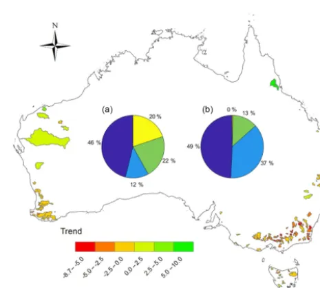
Out of the 217 catchments, about half of the catch-ments showed a significant decreasing trend, 37 % showed a significant decreasing trend, and 13 % showed a non-significant increasing trend (Fig. 2), detected using Mann– Kendall trend analysis (see Sect. 2.3). This is because Aus-tralia experienced the millennium drought over the period 2001–2009, which caused a dramatic streamflow reduction in this period (van Dijk et al., 2013). Trend analysis for the 217 catchments is explained in Sect. 2.3 and trend results are summarised in Sect. 3.
Out of the 217 catchments, about 46 % of catchments have no missing data in 1981–2010, 12 % with a missing data rate of <0.1 %, 22 % with a missing data rate of 0.1 %–0.5 %, and 20 % with a missing data rate of 0.5 %–1 % (Fig. 2).
To drive the two hydrological models, we obtained daily meteorological time series (including minimum
[image:2.612.311.545.67.283.2]tempera-Figure 1.The 780 unregulated catchments grouped by different streamflow data gaps for the period of 1981–2010.
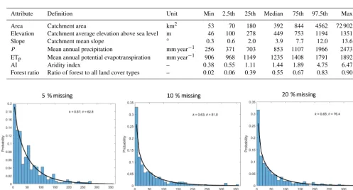
[image:2.612.311.544.335.544.2]Table 1.Major catchment attributes for the 217 catchments.
Attribute Definition Unit Min 2.5th 25th Median 75th 97.5th Max
Area Catchment area km2 53 70 180 392 844 4562 72 902 Elevation Catchment average elevation above sea level m 46 100 278 449 753 1194 1351 Slope Catchment mean slope ◦ 0.3 0.6 2.0 3.9 7.7 12.0 13.6 P Mean annual precipitation mm year−1 256 371 703 853 1107 1966 2473 ETp Mean annual potential evapotranspiration mm year−1 906 968 1149 1235 1408 1791 1892 AI Aridity index – 0.38 0.55 1.11 1.44 1.89 4.75 6.47 Forest ratio Ratio of forest to all land cover types – 0.02 0.06 0.39 0.55 0.67 0.83 0.90
Figure 3.Missing data patterns for three groups of catchments with missing data rates of 4 %–6 %, 8 %–12 %, and 18 %–22 %, which are represented by 5 %, 10 %, and 20 % missing data rates, respectively.
ture, maximum temperature, incoming solar radiation, ac-tual vapour pressure, and precipitation) from 1975 to 2012 at 0.05◦(∼5 km) grid resolution from the SILO Data Drill of the Queensland Department of Natural Resources and Wa-ter (https://silo.longpaddock.qld.gov.au/, last access on 8 Au-gust 2018). The data quality is reasonably good, indicated by the mean absolute error for maximum daily air temper-ature, minimum daily air tempertemper-ature, vapour pressure, and precipitation at 1.0◦C, 1.4◦C, 0.15 kPa, and 0.40 mm day−1 (Jeffrey et al., 2001).
2.2 Gap-filling experiments
For thoroughly investigating the potential impacts of infilled streamflow data on annual trend accuracy, we conducted three groups of experiments to test how the missing data rates at 5 %, 10 %, and 20 % impact streamflow trends. We followed three steps for each missing data rate of the experi-ments.
1. Missing data patterns were obtained using actual streamflow data.
We selected patterns of consecutive missing days from ac-tual data from the 780 catchments. For the 5 % group of miss-ing data rate experiments, we selected 44 catchments with missing rates of 4 %–6 %; for the 10 % group of missing data rate experiments, we selected 39 catchments with missing
data rates of 8 %–12 %; and for the 20 % group of missing data rate experiments, we selected 22 catchments with miss-ing data rates of 18 %–22 %. Figure 3 shows the probability distribution of consecutive missing days from each group of catchments, which is skewed toward the low end. We there-fore used the two-parameter Gamma distribution to simulate probability distribution of consecutive missing days (Fig. 3). The0distribution is expressed as
X∼0 (k, θ )=0(k, θ ), (1)
whereXis the number of consecutive missing days,kis the shape parameter, and θ is the scale parameter. The corre-sponding probability density function in the shape-scale pa-rameterisation is
f (x;k, θ )= 1 0(k)θkx
k−1e−x
θ, (2)
where0(k)is the gamma function.
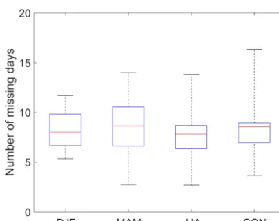
Figure 4.Distribution of number of missing days across different seasons, summarised from 39 catchments with a missing data rate ranging from 8 % to 12 % (i.e. 10 % missing data group).
to include more catchments in streamflow analyses. Thirdly, removing all periods of greater than 365 days allowed us to better fit a gamma distribution to the number of missing days. We also checked the seasonality of missing data to see if one season were more likely to have missing data than an-other. As seen from Fig. 4, the missing data are more or less evenly distributed through different seasons across all the 39 catchments (with a missing data rate of 8 % to 12 %) within the 10 % missing data group. This indicates that the data gaps were not skewed toward a particular season and they occurred randomly through the year.
2. Numbers of random consecutive missing days were gen-erated using a random number generator (sampling without replacement) based on the gamma distribution.
The random number generation was repeated 100 times to ensure the selected samples covered a wide range of stream-flow time series.
3. Streamflow data were gap-filled.
The selected days were treated as missing data and the un-selected data were used for hydrological model calibration. The missing data were then gap-filled using the simulated streamflow from the calibrated GR4J and SIMHYD models. For consistent interpretation hereafter, the benchmark streamflow data are regarded as “observed” and the experi-ment data as “filled”. For each of the three experiexperi-ments, there are 100×217 (21 700) missing data time series, with 100 rep-resenting sample times using the random number generator and 217 representing the number of catchments.
2.3 Trend analysis
We used the Mann–Kendall Tau-b non-parametric test in-cluding Sen’s slope method (Burn and Elnur, 2002) for an-nual streamflow trend analysis and significance testing for all three groups of experiments and benchmark data.
We used the following equation to quantify the trend bias:
Bt=Tfilled−Tobs, (3)
where Bt is the bias in the annual streamflow trend
(mm year−1year−1),Tfilled is the annual trend for gap-filled
streamflow (mm year−1year−1), andTobsis the annual trend
in observed streamflow (mm year−1year−1). It measures the trend error between the infilled and observed runoff trends withBt≈0, which indicates that the trend in observed
an-nual runoff is almost the same as that in the infilled anan-nual runoff.
We also defined relative trend bias (PBt) as
PBt=
Tfilled−Tobs Tobs
×100. (4)
2.4 Hydrological models
Two widely used hydrological models, SIMHYD and GR4J (Chiew et al., 2002, 2010; Li et al., 2014; Oudin et al., 2008; Perrin et al., 2003; Zhang and Chiew, 2009; Zhang et al., 2016a), were used to infill daily missing streamflow data. Both models require daily precipitation and daily potential evaporation (Priestley and Taylor, 1972) as model inputs, and model outputs are daily streamflow at each gauge. The daily inputs of the maximum and minimum temperatures, incom-ing solar radiation, and vapour pressure data were used to calculate the Priestley–Taylor daily potential evaporation.
The two models were calibrated using a global optimiser, consisting of a genetic algorithm (The MathWorks, 2006), at each catchment, with the first 6 years (i.e. 1975–1980) for spin-up and the remainder (1981–2010) for modelling exper-iments. Since this study mainly evaluates the trends obtained using the gap-filled streamflow from hydrological modelling, it is crucial to predict high flow and mean flow as accu-rately as possible. To this end, the model calibration was to minimise the following objective function (F) (Viney et al., 2009; Zhang et al., 2016b):
F =(1−NSE)+5|ln(1+B)|2.5, (5)
B=
N P
i=1
Qsim,i− N P
i=1 Qobs,i
N P
i=1 Qobs,i
, (6)
where NSE is the Nash–Sutcliffe efficiency of daily stream-flow,B is the model bias,Qsim andQobsare the simulated
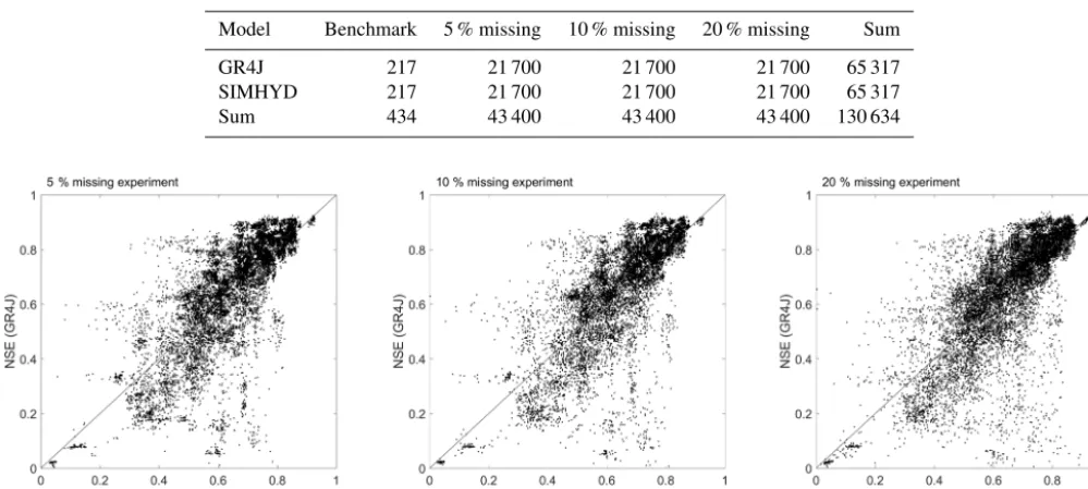
Table 2.Summary of model calibration number carried out for benchmark data and missing data experiments.
Model Benchmark 5 % missing 10 % missing 20 % missing Sum
GR4J 217 21 700 21 700 21 700 65 317
SIMHYD 217 21 700 21 700 21 700 65 317
Sum 434 43 400 43 400 43 400 130 634
Figure 5.Comparisons between calibrated GR4J and calibrated SIMHYD for 44 catchments of the 5 % missing data experiment, 39 catch-ments of the 10 % missing data experiment, and 22 catchcatch-ments of the 20 % missing data experiment. In each catchment, there were 100 replicates carried out.
modelled daily streamflow, withB=0 indicating that the av-erage of modelled daily streamflow is the same as the avav-erage of observed daily streamflow.
For each catchment, GR4J and SIMHYD were calibrated using benchmark data and 100 time series of streamflow data with missing data (see Sect. 2.2), respectively. For bench-mark data without any missing data (46 % catchments), no gap filling is required; for the benchmark data with missing data rates less than 1 %, the calibrated continuous stream-flow data were used to fill the gaps. For the missing data experiments, the calibrated continuous streamflow data for each missing replicate were used to infill the artificially made missing data. Table 2 summarises the model calibrations car-ried out for the benchmark and for each experiment. Finally, 130 634 model calibrations and 130 200 times of gap fill-ing were carried out. Finally, the trends estimated from the benchmark were used to evaluate those obtained from the missing data experiments.
3 Results
The gap-filled data from the two hydrological models were evaluated against the benchmark data. Overall, the two mod-els perform well and neither significantly outperforms the other (Fig. 5). For the three groups of gap-filling experi-ments, these two models perform similarly (i.e. the difference of NSE of daily runoff between the two is less than 0.02) in 18 %–19 % catchments; the SIMHYD model outperforms
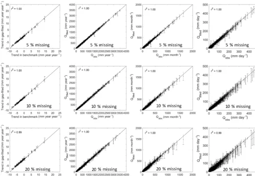
the GR4J model (NSE difference between the two is larger than 0.02) in 30 %–31 % catchments; and the GR4J model outperforms the SIMHYD model in 50 %–51 % catchments. Figures 6 and 7 summarise the performance of the gap-filled data for estimating annual trends, annual streamflow, monthly streamflow, and daily streamflow, respectively. The three missing data rate experiments (5 %, 10 %, and 20 %) perform almost the same as the benchmark (Figs. 6 and 7). The coefficient of determination (r2) between the gap-filled trends and observed trends is more than 0.98 for the three experiments and two hydrological models.
Since errors in gap-filled trends are likely to be different and time steps are different when daily infilled streamflow data are used, we further investigate how gap-filled errors are propagated from daily to monthly and to annual scales in the three gap-filling cases (5 %, 10 %, and 20 %) (Figs. 6 and 7). It is expected that daily gap-filled streamflow has a larger standard deviation from the benchmark than monthly and annual streamflow since the streamflow was gap-filled at a daily scale. This indicates that the temporal aggregation smooths the gap-filled error strongly, and it generates very reasonable monthly and annual streamflow estimates with less standard deviation. It is interesting to note that both mod-els tend to underestimate very high flows, though they are calibrated against the NSE of daily streamflow, which gives larger weight to the correct representation of higher flows.
pos-Figure 6.Comparisons between the observed streamflow (xaxis) and gap-filled ones (yaxis) for streamflow trend (mm year−1year−1, left panels), annual streamflow (mm year−1, second left panels), monthly streamflow (mm month−1, second right panels), and daily streamflow (mm day−1, right panels). The gaps were filled using GR4J. The error bar represents standard deviation of the 100 replicates for each group of missing data experiments.
itive to negative). For the experiments with 5 % and 10 % missing data rates and for GR4J, fewer than 8 out of the 217 catchments show a trend mismatch, and almost all of them show non-significant trends (p >0.05). For the experiments with a 20 % missing data rate for GR4J, fewer than 10 out of the 217 catchments show a trend mismatch, and all of them show non-significant trends. SIMHYD results are al-most the same as GR4J results. All these indicate that there is very marginal influence on annual streamflow trend direc-tions when the missing data rate is less than 20 %.
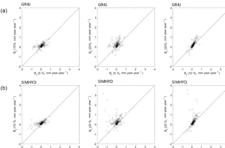
Though the three groups of experiments show small trend direction changes (Fig. 8), it is not clear how the trend bias (Eq. 3) looks. To this end, Fig. 9 further compares the trend bias between the experiments. It is clear that the trend biases between 5 % and 10 % missing data experi-ments are similar. For GR4J, both have a trend bias vary-ing from−1 to 1 mm year−1year−1. For SIMHYD, the trend bias between the two is similar when it varies from−0.5 to 1 mm year−1year−1, and the trend bias of the 5 % missing
data experiment is even larger than that of the 10 % missing data experiment. The trend bias of the 20 % missing data ex-periment is noticeably larger than that of the 10 % and 5 % missing data experiments for both models, and the underper-formance is more noticeable in the SIMHYD gap-filled data than in the GR4J gap-filled data. This result suggests that the trend bias is reasonable when the missing data rate is less than 10 %, and can be large for a small number of catchments when the missing data rate is up to 20 %.
4 Discussion and conclusions
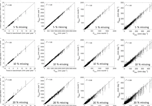
[image:6.612.50.548.66.410.2]Figure 7.Same as Fig. 6 but using SIMHYD.
many more catchments in modelling and data analysis stud-ies. For example, of the 780 unregulated Australian catch-ments available for modelling studies (Zhang et al., 2013), there are 237 catchments with a missing data rate of 1 %– 10 % during 1981–2010, accounting for 38 % of total avail-able catchments (Fig. 1). Of these 237, 67 (∼28 %) also have gaps lasting more than 1 year (which we did not consider in this analysis), and therefore these may not be suitable for use. With an increased number of catchments, more reliable large-scale hydrological modelling studies can be carried out (Beck et al., 2016; Parajka et al., 2013; Zhang et al., 2016a). The missing rate experiments designed in this study are based on the actual missing data patterns obtained from the 780 catchments. In most cases, the number of consecutive missing days is less than 10, as indicated by Fig. 3, indicating brief periods of gauge malfunctions. It is, however, interest-ing to note that there are streamflow gaps lastinterest-ing much longer than this in many catchments, with gaps of many months in some cases, noting that we excluded gaps lasting 1 year or more. It is highly likely that filling a gap of 1 year or more will result in biases larger than those presented here.
Furthermore, we also tested the quality of random gap-filled daily streamflow. In that case, the missing data patterns were randomly selected using a random number generator. The results obtained from the random gap filling (not shown) are similar to the results presented here. Thus, it is likely that the length of the gaps (as long as it is less than 1 year) is unlikely to impact the results of the gap-filling experiment. We conclude from this that the use of hydrologic modelling for filling the substantially gapped data (up to a 10 % missing data rate) described here for Australia will not impact annual trends of streamflow. Impacts on other streamflow character-istics also need to be examined, as well as seeing if the results obtained in Australia are comparable with those in other parts of the world, where the length of observational gaps may be quite different to those shown in Fig. 3.
Figure 8.Trend mismatch analysis between the gap-filled and benchmark data. “Total” refers to all the mismatch catchments, “N” denotes non-significant trends (p >0.05), and “S” denotes significant trends (p≤0.05). The bottom, middle, and top of each box show the 25th, 50th, and 75th percentiles, and the bottom and top whiskers are the 5th and 95th percentiles.
flow (>95th percentile) or low flow (<50th percentile) data. The results obtained from the low flow gap filling indicates that there is only a negligible influence on annual streamflow trend estimates when the missing data rate is less than 50 %. In contrast, the high flow gap-filled data show a noticeable change in annual streamflow trend when the missing data rate is 5 %. This is understandable since high flow is usually sev-eral orders of magnitude higher than low flow, and errors in filling high flow could have large impacts on annual flow and its trends (Slater and Villarini, 2017).
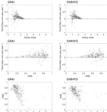
To understand if the quality of gap-filled streamflow is related to catchment attributes and calibration accuracy, we conducted further analysis among the trend bias, model cal-ibration efficiency (i.e. NSE), and catchment aridity index (mean annual potential evaporation divided by mean annual precipitation) (Fig. 10). The model calibration results in dry catchments are normally poorer than those in wet catch-ments. However, the trend bias (mm year−1year−1) obtained from dry catchments is usually smaller. The large biases are observed from the catchments with an aridity index less than 2 and with the calibrated NSE being larger than 0.60. In part, this is to be expected since the streamflow is also lower in more arid catchments, meaning that the trend bias is also likely to be lower.
Figure 11 shows the relationship between the relative trend bias (%, Eq. 4) and aridity index. It shows that not only is the actual trend bias lower in drier catchments, but so too is the relative (%) trend. This result suggests that the large bias in annual trends as a result of gap filling is observed in rela-tively wet catchments, where model calibrations are reason-ably good. This result seems counter-intuitive and requires further exploration, which is beyond the scope of the current paper.
Figure 9.Trend biases comparison between the three groups of gap-filling experiments (5 %, 10 % and 20 %).(a)is for GR4J and(b)is for SIMHYD.
the direct low flow metrics. Another possible method is to combine hydrological modelling with other methods of gap filling, such as using nearby gauges (Lopes et al., 2016) and statistical methods (Gedney et al., 2006b).
It is noted that the infilled data purely refer to the miss-ing data. All streamflow gauges only measure to a certain flow. Once the flow exceeds that level during flooding, the results are interpolated using stage–discharge relationships (Peña-Arancibia et al., 2015). These interpolations could be a major source of observation error. However, investigating high flow interpolation and data quality is beyond the scope of this study.
The modelling experiments and findings from this study could have important implications for other parts of the world as well as Australia. First, to develop appropriate gap-filling modelling experiments, it is necessary to evaluate the tribution of consecutive missing data. The probability dis-tribution of consecutive missing data is skewed toward the low end, which can be nicely simulated using the gamma distribution (Eq. 1). This distribution should be very use-ful for similar missing data patterns in other regions. Sec-ond, hydrological modelling is a very good tool for filling gaps since it can fully take advantage of climate forcing and non-gap streamflow data and obtain the best possible daily simulations. Third, the threshold of 10 % identified in this
study should be applicable to regions/catchments with simi-lar missing data patterns. However, if the data gaps continue for seasons or years, the threshold may not hold.
It would also be interesting to compare hydrological mod-elling to other approaches for filling streamflow data gaps. Hydrological modelling is a most useful method used in Aus-tralia for predicting daily streamflow in ungauged catchments (Chiew et al., 2009; Li and Zhang, 2017; Zhang and Chiew, 2009; Viney et al., 2009). It has been used operationally by the Australian Bureau of Meteorology for filling daily streamflow data gaps for many years. In the future, this oper-ational method could further be comprehensively evaluated against other approaches, such as interpolation or correlation with nearby gauging sites.
catch-Figure 10.Relationships among trend bias (mm year−1year−1), model calibration Nash–Sutcliffe efficiency and aridity index for each catchment and for the experiment of the 10 % missing data rate.
[image:10.612.124.471.500.679.2]ments appears to be more successful than gap-filling wetter catchments.
Data availability. Streamflow data used in this study are
available at https://doi.org/10.4225/08/58b5baad4fcc2. The modelling experiment data are freely available upon request from the corresponding author (Yongqiang Zhang, email: [email protected]).
Author contributions. YQZ conceived this study and conducted
modelling experiments and data analysis. YQZ finished the first draft and DP modified it. YQZ and DP addressed comments from reviewers.
Competing interests. The authors declare that they have no conflict
of interest.
Acknowledgements. This study was supported by the CSIRO
strategic project “Next generation methods and capability for multi-scale cumulative impact assessment”. The authors thank constructive suggestions from the editor, Louse Slater, and two reviewers, Maxine Zaidman and Juraj Parajka.
Edited by: Louise Slater
Reviewed by: Maxine Zaidman and Juraj Parajka
References
Beck, H. E., van Dijk, A. I. J. M., de Roo, A., Mi-ralles, D. G., McVicar, T. R., Schellekens, J., and Brui-jnzeel, L. A.: Global-scale regionalization of hydrologic model parameters, Water Resour. Res., 52, 3599–3622, https://doi.org/10.1002/2015wr018247, 2016.
Burn, D. H. and Elnur, M. A. H.: Detection of hydrologic trends and variability, J. Hydrol., 255, 107–122, 2002.
Chiew, F. H. S., Peel, M. C., and Western, A. W.: Application and testing of the simple rainfall-runoff model SIMHYD, in: Math-ematical Models of Small Watershed Hydrology and Applica-tions, edited by: Singh, V. P. and Frevert, D. K., Water resources Publication, Littleton, Colorado, USA, 335–367, 2002. Chiew, F. H. S., Teng, J., Vaze, J., Post, D. A., Perraud, J. M.,
Kirono, D. G. C., and Viney N. R.: Estimating climate change impact on runoff across southeast Australia: Method, results, and implications of the modeling method, Water Resour. Res.. 45, W10414, https://doi.org/10.1029/2008WR007338, 2009. Chiew, F. H. S., Kirono, D. G. C., Kent, D. M., Frost, A. J., Charles,
S. P., Timbal, B., Nguyen, K. C., and Fu, G.: Comparison of runoff modelled using rainfall from different downscaling meth-ods for historical and future climates, J. Hydrol., 387, 10–23, https://doi.org/10.1016/j.jhydrol.2010.03.025, 2010.
Dai, A., Qian, T., Trenberth, K. E., and Milliman, J. D.: Changes in Continental Freshwater Discharge from 1948 to 2004, J. Climate, 22, 2773–2792, https://doi.org/10.1175/2008jcli2592.1, 2009.
Déry, S. J., Hernández-Henríquez, M. A., Burford, J. E., and Wood, E. F.: Observational evidence of an intensifying hydro-logical cycle in northern Canada, Geophys. Res. Lett., 36, 1–5, https://doi.org/10.1029/2009gl038852, 2009.
Gedney, N., Cox, P. M., Betts, R. A., Boucher, O., Huntingford, C., and Stott, P. A.: Detection of a direct carbon dioxide ef-fect in continental river runoff records, Nature, 439, 835–838, https://doi.org/10.1038/nature04504, 2006a.
Gedney, N., Cox, P. M., Betts, R. A., Boucher, O., Hunting-ford, C., and Stott, P. A.: Continental runoff – A quality-controlled global runoff data set – Reply, Nature, 444, E14–E15, https://doi.org/10.1038/nature05481, 2006b.
Hannaford, J. and Buys, G.: Trends in seasonal river flow regimes in the UK, J. Hydrol., 475, 158–174, https://doi.org/10.1016/j.jhydrol.2012.09.044, 2012.
Harvey, C. L., Dixon, H., and Hannaford, J.: An appraisal of the performance of data-infilling methods for application to daily mean river flow records in the UK, Hydrol. Res., 43, 618–636, https://doi.org/10.2166/nh.2012.110, 2012.
Jeffrey, S. J., Carter, J. O., Moodie, K. B., and Beswick, A. R.: Us-ing spatial interpolation to construct a comprehensive archive of Australian climate data, Environ. Model. Softw., 16, 309–330, 2001.
Lavers, D., Prudhomme, C., and Hannah, D. M.: Large-scale cli-mate, precipitation and British river flows Identifying hydrocli-matological connections and dynamics, J. Hydrol., 395, 242– 255, https://doi.org/10.1016/j.jhydrol.2010.10.036, 2010. Li, F., Zhang, Y., Xu, Z., Liu, C., Zhou, Y., and Liu,
W.: Runoff predictions in ungauged catchments in southeast Tibetan Plateau, J. Hydrol., 511, 28–38, https://doi.org/10.1016/j.jhydro1.2014.01.014, 2014.
Li, H. and Zhang, Y.: Regionalising rainfall-runoff mod-elling for predicting daily runoff: Comparing gridded spa-tial proximity and gridded integrated similarity approaches against their lumped counterparts, J. Hydrol., 550, 279–293, https://doi.org/10.1016/j.jhydrol.2017.05.015, 2017.
Liu, J. and Zhang, Y.: Multi-temporal clustering of continental floods and associated atmospheric circulations, J. Hydrol., 555, 744–759, https://doi.org/10.1016/j.jhydrol.2017.10.072, 2017. Lopes, A. V., Chiang, J. C. H., Thompson, S. A., and Dracup, J.
A.: Trend and uncertainty in spatial-temporal patterns of hydro-logical droughts in the Amazon basin, Geophys. Res. Lett., 43, 3307–3316, https://doi.org/10.1002/2016gl067738, 2016. Mackay, S. J., Arthington, A. H., and James, C. S.:
Classifica-tion and comparison of natural and altered flow regimes to support an Australian trial of the Ecological Limits of Hy-drologic Alteration framework, Ecohydrology, 7, 1485–1507, https://doi.org/10.1002/eco.1473, 2014.
Oudin, L., Andreassian, V., Perrin, C., Michel, C., and Le Moine, N.: Spatial proximity, physical similarity, regression and ungaged catchments: A comparison of regionalization approaches based on 913 French catchments, Water Resour. Res., 44, W03413, https://doi.org/10.1029/2007WR006240, 2008.
Peña-Arancibia, J. L., Zhang, Y., Pagendam, D. E., Viney, N. R., Lerat, J., van Dijk, A. I. J. M., Vaze, J., and Frost, A. J.: Stream-flow rating uncertainty: Characterisation and impacts on model calibration and performance, Environ. Model. Softw., 63, 32–44, https://doi.org/10.1016/j.envsoft.2014.09.011, 2015.
Perrin, C., Michel, C., and Andreassian, V.: Improvement of a parsi-monious model for streamflow simulation, J. Hydrol., 279, 275– 289, https://doi.org/10.1016/s0022-1694(03)00225-7, 2003. Petrone, K. C., Hughes, J. D., Van Niel, T. G., and Silberstein, R. P.:
Streamflow decline in southwestern Australia, 1950–2008, Geo-phys. Res. Lett., 37, 1–7, https://doi.org/10.1029/2010gl043102, 2010.
Priestley, C. H. B. and Taylor, R. J.: On the assessment of surface heat flux and evaporation using large-scale parameters, Mon. Weather Rev., 100, 81–92, 1972.
Pushpalatha, R., Perrin, C., Le Moine, N., and Andreas-sian, V.: A review of efficiency criteria suitable for eval-uating low-flow simulations, J. Hydrol., 420, 171–182, https://doi.org/10.1016/j.jhydrol.2011.11.055, 2012.
Rojas-Serna, C., Lebecherel, L., Perrin, C., Andreassian, V., and Oudin, L: How should a rainfall-runoff model beparam-eterized in an almost ungaugedcatchment? A methodology tested on 609 catchments, Water Resour. Res., 52, 4765–4784, https://doi.org/10.1002/2015WR018549, 2016.
Sanderson, M. G., Wiltshire, A. J., and Betts, R. A.: Projected changes in water availability in the United Kingdom, Water Re-sour. Res., 48, W08512, https://doi.org/10.1029/2012wr011881, 2012.
Seibert, J. and Beven, K. J.: Gauging the ungauged basin: how many discharge measurements are needed?, Hydrol. Earth Syst. Sci., 13, 883–892, https://doi.org/10.5194/hess-13-883-2009, 2009. Slater, L. and Villarini, G.: On the impact of gaps on trend detection
in extreme streamflow time series, Int. J. Climatol., 37, 3976– 3983, https://doi.org/10.1002/joc.4954, 2017.
Smakhtin, V. U.: Low flow hydrology: a review, J. Hydrol., 240, 147–186, https://doi.org/10.1016/s0022-1694(00)00340-1, 2001.
Staudinger, M., Stahl, K., Seibert, J., Clark, M. P., and Tallaksen, L. M.: Comparison of hydrological model structures based on recession and low flow simulations, Hydrol. Earth Syst. Sci., 15, 3447–3459, https://doi.org/10.5194/hess-15-3447-2011, 2011. The MathWorks, Inc.: Genetic algorithm and direct search toolbox
2 user’s guide, Natick, Mass, 5.2–5.13, 2006.
Ukkola, A. M., Prentice, I. C., Keenan, T. F., van Dijk, A. I. J. M., Viney, N. R., Myneni, R. B., and Bi, J.: Re-duced streamflow in water-stressed climates consistent with CO2 effects on vegetation, Nat. Clim. Change, 6, 75–78, https://doi.org/10.1038/nclimate2831, 2015.
Ukkola, A. M., Keenan, T. F., Kelley, D. I., and Pren-tice, I. C.: Vegetation plays an important role in mediat-ing future water resources, Environ. Res. Lett., 11, 094022, https://doi.org/10.1088/1748-9326/11/9/094022, 2016.
van Dijk, A. I. J. M., Beck, H. E., Crosbie, R. S., de Jeu, R. A. M., Liu, Y. Y., Podger, G. M., Timbal, B., and Viney, N. R.: The Mil-lennium Drought in southeast Australia (2001–2009): Natural and human causes and implications for water resources, ecosys-tems, economy, and society, Water Resour. Res., 49, 1040–1057, https://doi.org/10.1002/wrcr.20123, 2013.
Viney, N. R., Perraud, J., Vaze, J., Chiew, F. H. S., Post, D. A., and Yang, A.: The usefulness of bias constraints in model cali-bration for regionalisation to ungauged catchments, 18th World IMACS Congress and Modsim09 International Congress on Modelling and Simulation: Interfacing Modelling and Simula-tion with Mathematical and ComputaSimula-tional Sciences, Cairns, Australia, 13–17 July 2009, 3421–3427, 2009.
Yang, Y., McVicar, T. R., Donohue, R. J., Zhang, Y., Roderick, M. L., Chiew, F. H. S., Zhang, L., and Zhang, J.: Lags in hydrologic recovery following an extreme drought: Assessing the roles of climate and catchment characteristics, Water Resour. Res., 53, 4821–4837, https://doi.org/10.1002/2017wr020683, 2017. Zhang, Y. and Chiew, F. H. S.: Relative merits of different methods
for runoff predictions in ungauged catchments, Water Resour. Res., 45, W07412, https://doi.org/10.1029/2008WR007504, 2009.
Zhang, Y., Vaze J., Chiew, F. H. S., Teng, J., and Li, M.: Predict-ing hydrological signatures in ungauged catchments usPredict-ing spa-tial interpolation, index model, and rainfall–runoff modelling, J. Hydrol., 517, 936–948, 2014.
Zhang, Y., Pena-Arancibia, J. L., McVicar, T. R., Chiew, F. H., Vaze, J., Liu, C., Lu, X., Zheng, H., Wang, Y., Liu, Y. Y., Mi-ralles, D. G., and Pan, M.: Multi-decadal trends in global terres-trial evapotranspiration and its components, Sci. Rep., 6, 19124, https://doi.org/10.1038/srep19124, 2016a.
Zhang, Y., Zheng, H., Chiew, F. H. S., Pena-Arancibia, J., and Zhou, X.: Evaluating Regional and Global Hydrological Models against Streamflow and Evapotranspiration Measurements, J. Hydrome-teorol., 17, 995–1010, https://doi.org/10.1175/jhm-d-15-0107.1, 2016b.