Benjamin Hofner, Torsten Hothorn and Thomas Kneib
Variable Selection and Model Choice in
Structured Survival Models
Technical Report Number 043, 2008 Department of Statistics
University of Munich
Variable Selection and Model Choice in Structured Survival Models
Benjamin Hofner∗ Torsten Hothorn† Thomas Kneib†Abstract
In many situations, medical applications ask for flexible survival models that allow to extend the classical Cox-model via the inclusion of time-varying and nonparametric effects. These structured survival models are very flexible but additional difficulties arise when model choice and variable selection is desired. In particular, it has to be decided which covariates should be assigned time-varying effects or whether parametric modeling is sufficient for a given covariate. Component-wise boosting provides a means of likelihood-based model fitting that enables simultaneous variable selection and model choice. We introduce a component-wise likelihood-based boosting algorithm for survival data that permits the inclusion of both parametric and nonparametric time-varying effects as well as nonparametric effects of continuous covariates utilizing penalized splines as the main modeling technique. Its properties and performance are investigated in simulation studies. The new modeling approach is used to build a flexible survival model for intensive care patients suffering from severe sepsis. A software implementation is available to the interested reader.
Key words: likelihood-based boosting, hazard regression, model choice, P-splines, smooth effects, time-varying effects
1 Introduction
Classical survival models had a break-through with the well-known, omnipresent Cox model [1], where the hazard rate is described in terms of a baseline hazard and multiplicative covariate effects. Mod-eling more complex survival regression relationships requires a more flexible model structure and in particular calls for smooth, nonlinear and time-varying effects. Here, we focus on building a model for the survival time of intensive care patients suffering from severe sepsis. Previously published findings, based on survival models estimated for 462 patients which were enrolled in a study initiated at the university hospital “Klinikum Großhadern” of the Ludwig-Maximilians-Universit¨at M¨unchen, suggest that out of potentially 20 covariates, 14 covariates have an impact on the survival time or were set as mandatory covariates [2]. The model was derived based on the recently developed two-stage stepwise
procedure of Hofner et al. [3]. To illustrate the type of models we will consider in the following, we
chose three exemplary covariates of the 14 covariates that were identified to have an impact on survival
times: “age” (x1) was selected as linear term, “Apache II score” (x2, a measure for the severity of
disease determined within the first 24 hours of admission) had a smooth effect and “fungal infection”
(x3) was modeled with time-varying effect. In other words, the following structured, flexible survival
model for the hazard rate has to be fitted
λ(t|x) =λ0(t) expflinear(x1) +fsmooth(x2) +fsmooth(t)·x3 , (1)
where x = (x1, x2, x3)> is the vector of covariates, λ0(t) represents the baseline hazard, flinear(x1)
is a linear function of “age” (x1), fsmooth(x2) is a smooth function of “Apache II score” (x2), and
∗Institut f¨ur Medizininformatik, Biometrie und Epidemiologie, Friedrich-Alexander-Universit¨at Erlangen-N¨urnberg,
Waldstraße 6, 91054 Erlangen, Germany; Email: [email protected]
fsmooth(t) is again a function of time t, which represents the time-varying effect of “fungal infection”
(x3). Once one is sure about the principle structure of such a complex model, various approaches to
model fitting can be applied. Basics of Cox-type additive models can be found, e.g., in Zucker and
Karr [4] or Fahrmeir et al.[5]. Hastie and Tibshirani [6] introduced models with varying-coefficients
and also considered time-varying effects in Cox models as a specific example. Time-varying effects can
be expressed as the product of a P-spline and the covariate (e.g., [7]). This can be seen infsmooth(t)·x3,
where fsmooth(t) is modeled using P-splines. The smooth function fsmooth(x2) can also be modeled
using P-splines.
However, the crucial point is not simply fitting a model similar to (1) but to derive a model structure describing the response in terms of only influential covariates at an appropriate complexity.
In model (1), one might ask why a smooth term for x2 is required whereas a simple linear term seems
to be sufficient to capture the impact of x1. In principle, we have to decide what the appropriate
complexity (linear effect, smooth effect or time-varying effect) for each variable is. This decision has to be based on data and thus we are faced with a model choice problem. Even more crucial is the necessity to distinguish between influential and non-influential covariates. A covariate is influential if it is related to the response in any of the given modeling possibilities and non-influential if it is independent of the response. Thus, in addition to the model choice problem, we are faced with a variable selection problem and need not only to select variables but also to determine the appropriate structure for the covariate at the same time.
In classical structured Cox-type additive models it is hard to deal with both the model choice and variable selection problem. It is often not clear if a covariate should enter the model as linear term, smooth term or as time-varying effect, or even not enter the model at all. One approach to address this problem are multivariable fractional polynomials [8]. The basic idea is to start with the simplest model and to apply an iterative variable inclusion procedure based on a series of tests for inclusion of variables and for determining the complexity of the functional form. A two-stage stepwise variable selection and model choice algorithm for structured Cox-type additive models based on information
criteria (as e.g., AIC or BIC) is suggested by Hofner et al. [3] and was applied to model the severe
sepsis data. Other approaches that are based on hypothesis tests may be applied as well [9]. These and similar multi-step procedures perform a series of locally optimal fit and selection procedures, however, the quality of the global model fit can only be investigated empirically.
To overcome these conceptual and associated practical problems, we propose a one-step model fitting approach with intrinsic variable selection and model choice within the framework of empirical risk minimization. Our suggestion is to fit structured survival models with potentially many covariates by minimizing the respective negative (log)-likelihood based on boosting techniques. More specifically, a component-wise boosting approach is applied which allows for estimation of structured models and has been shown to lead to final models containing influential variables at appropriate complexity, for example in [10]. Over the last twelve years, an extensive amount of literature has been devoted to boosting techniques and we therefore refer the reader to B¨uhlmann and Hothorn [11] for an overview.
In a context not unlike the one dealt with in this paper, Kneibet al.[12] studied boosting techniques for
estimation, variable selection and model choice for spatially structured exponential family regression models.
The rest of the paper is organized as follows: Structured survival models and penalized likelihood estimation schemes that will be utilized as building blocks in the boosting algorithm are introduced in Section 2. Section 3 a component-wise, likelihood-based boosting method that allows for simultaneous model choice and estimation. A simulation study to investigate the characteristics of the algorithm is given in Section 4. The application of the algorithm to the severe sepsis data, as briefly introduced above, is also presented in this section, along with an empirical comparison with the two-stage stepwise
selection procedure by Hofner et al. [3]. Section 5 contains a discussion of the proposed method and
2 Structured Survival Models
To overcome the restrictions of Cox models, as discussed above, we allow the inclusion of both, time-varying and smooth effects. For methodological considerations take a generic, structured survival model
λ(t|xi) = exp(ηi(xi)), i= 1, . . . , n, (2)
with an additive predictor of the form
ηi(xi) =β0+
J X j=1
fj(xi), (3)
where the functionsfj(xi) are a generic representation of different types of covariate effects. To make
the model formulation (3) more concrete, consider the following examples of functions fj(x): The
functions can represent linear effects fj(x) = flinear(˜x) = ˜xβ, where ˜x is a univariate element of x,
smooth effects fj(x) =fsmooth(˜x), where ˜xis a univariate, continuous covariate from xandfsmooth is
a smooth function, andtime-varying effectsfj(x) =fsmooth(t)·x˜, where the vector (˜x, t) is included in
x. The covariate ˜xcan be either continuous or categorical,trepresents the observed survival time and
fsmooth is again a smooth function. The log-baseline hazard can be specified in the additive predictor
(3) as a special form of the generic functions, i.e., fj = fsmooth(t) = log(λ0(t)). Thus, there is no
need to additionally specify the classical baseline hazardλ0(t) in the model (2). Furthermore, the full
likelihood is available and thus can be used for inference.
The smooth functionsfsmooth, of ˜x as well as of timet, can be modeled, for example, by applying
fractional polynomials [13, 14]. Perperoglouet al. [15] propose the reduced-rank regression model to
model time-varying effects based on B-splines. Both, flexible and time-varying effects can be modeled by classical smoothers as regression splines, smoothing splines [7] or P-splines. The latter where introduced by Eilers and Marx [16] based on B-splines [17], where smooth functions are modeled using a parametric analogon fsmooth(˜x) = M X m=1 βmBm(˜x). (4)
The B-spline basis functions Bm(˜x) are defined over an equidistant grid ofM knots. The coefficients
βm become part of the vector of unknown parameters we want to estimate. An additional penalty for
higher order differences of coefficientsβm for adjacent knots is used to achieve smooth estimates. For
the j-th function fj(x˜) = fsmooth(x˜), we get the parameter vector βpen,j = (β1,j, . . . , βM,j)> and the
design matrix Xpen,j = (B1,j(x˜), . . . , BM,j(x˜)), where x˜ is the covariate vector corresponding to the
j-th generic function. Numerically, P-splines are very stable and the computational effort is reduced
compared to, e.g., smoothing splines. In the survival context, P-splines are frequently used to model smooth functions [18]. Schmid and Hothorn [19] showed that P-splines can also be successfully used in the boosting context. They reason that the computational effort is heavily decreased and the predictive performance is only marginally effected when using P-splines instead of smoothing splines. Following this argumentation we use P-splines as base-learners for flexible model terms in the remainder of this paper.
To estimate the structured, flexible survival model, we need to derive the penalized components for likelihood estimation in this context. The likelihood will then be maximized by applying a
component-wise boosting approach. Letti denote the observed survival time of thei-th observation (i= 1, . . . , n)
log-likelihood can be expressed as lpen(β) = n X i=1 δiηi− Z ti 0 λi(˜t)d ˜ t − J X j=1 κj 2 βpen> ,jKjβpen,j =hδ>η−1>Λi−12β>Kβ (5) =l(β)−12β>Kβ, where β> = (β>
pen,1, . . . ,βpen> ,J,γ>) is the parameter vector,Λ = (Λ1(t1), . . . ,Λn(tn))> is the vector
of the cumulative hazard rates Λi(ti) = R0tiλi(˜t)d˜t, l(β) denotes the unpenalized log-likelihood and
K = diag(κ1K1, . . . , κJKJ,0) is a block diagonal matrix representing the penalization. Kj is a
differ-ence matrix (classically of order two) for the j-th component and κj is the corresponding smoothing
parameter. The latter determines the smoothness of the resulting function estimate, where bigger
values ofκj correspond to smoother functions andκj = 0 corresponds to an unpenalized estimation of
the j-th term. Note that the smoothing parameters κj, j = 1, . . . , J are part ofK and linear effects
remain unpenalized in the model, only coefficients corresponding to smooth terms are penalized.
The score vector is given by the first derivative of the (penalized) log-likelihoodlpen(β)
spen(β) = ∂∂βlpen(β) = " δ>X−Xn i=1 Z ti 0 xi(˜t)λi(˜t)d ˜ t # −Kβ (6) =s(β)−Kβ,
where the unpenalized score function is denoted by s(β). The notation xi(˜t) depicts that xi may
contain time-depending covariates. This can, for example, be the case when time-varying effects are used, as these are expressed as artificial time-dependent covariates. The penalized, observed Fisher matrix is then calculated as the negative second derivative of the penalized log-likelihood:
Fpen(β) =− ∂ 2 ∂β∂β>lpen(β) = " n X i=1 Z ti 0 xi(˜t)x > i (˜t)λi(˜t)d˜t # +K (7) =F(β) +K.
The Fisher matrix that results from unpenalized estimation is given asF(β). With these formulations
at hand one can estimate the parameters using Fisher scoring or any other numerical optimization method.
In most cases it is better to define the smoothness of a function using the effective degrees of freedom
df than to set the smoothing parameters κj, j = 1, . . . , J itself. This makes functions comparable
w.r.t. their flexibility (i.e. smoothness) and is more intuitive. Gray [7] derived the degrees of freedom in flexible survival models with penalized splines as
df := traceF ·Fpen−1. (8)
Note that the degrees of freedom depend on the smoothing parametersκj, j= 1, . . . , J, the parameters
3 Boosting in Survival Models with Time-Varying Effects
In this section, we device an estimation procedure for Cox-type models with additive structure and possibly time-varying effects. Variable selection and model choice play another major role in this setting. To combine all tasks, component-wise boosting methods are applied in the following.
3.1 Basic Considerations
Estimation of models can be done with respect to many different criteria. In the boosting context, minimization of a loss function based on the negative gradient (functional gradient descent [FGD] boosting) or direct maximization of a likelihood-based criterion (likelihood-based boosting) is usually
applied. We restrict to the latter case and base the estimation on thefull log-likelihood (in contrast to
the usually applied partial log-likelihood). Likelihood-based boosting directly aims to maximize the log-likelihood and thus is to be understood as a special algorithm for the maximization of the likelihood. Boosting is based on base-learners, i.e., functions that lead to (typically) small improvements of the estimation in each boosting iteration. Thus, we are slowly approaching a solution. For more details on base-learners in general and on how to choose them we refer to B¨uhlmann and Hothorn [11]. In the following, we will consider linear and P-spline base-learners. For the latter base-learners, the optimization criterion is altered from the unpenalized to the penalized log-likelihood as given in (5).
Variable Selection To incorporate variable selection, component-wise boosting [10] is employed. For each covariate a separate base-learner is specified and only the best fitting base-learner (w.r.t. some criterion) is updated in each iteration. Hence, classically we do not incorporate each base-learner in the model before we reach the “optimal” boosting iteration, which means that variable selection is performed.
Model Choice To incorporate model choice in the (component-wise) boosting framework we add separate base-learners for each modeling possibility. A variable can then be added in any of the modeling possibilities, which corresponds to model choice. Furthermore, a variable is considered to be
selected if any of the modeling possibilities is chosen. Thus, we have a variable selection and model
choice approach based on component-wise boosting.
From the generic, flexible survival model (2, 3) we see that a covariate ˜xican enter the model in up
to three different ways. The effect can be either linear, smooth (in the case of a continuous covariate ˜
xi) or time-varying. Hence, the question arises, how each variable should enter the model. One
solution is, to specify a separate base-learner for each suitable modeling possibility. Component-wise boosting then chooses between covariates and modeling possibilities at the same time, if the boosting algorithm is stopped after an appropriate number of iterations. Linear effects enter the model as linear base-learners, smooth effects can be added using P-spline base-learners and time-varying effects are
derived as a base-learner for the interaction between a P-spline of time and the covariate ˜xi.
To make the different base-learners comparable in terms of complexity, one could try to define
equal degrees of freedom for each term. Increasing the smoothing parameter κ leads to decreasing
degrees of freedom. However, Eilers and Marx [16] showed that a polynomial of order d−1 remains
unpenalized by a d-th order difference penalty if the degree of the B-spline basis is larger or equal
thand−1. Thus, we cannot make the degrees of freedom arbitrary small. As classically we are using
B-splines of degree 3 or higher, the degrees of freedom for difference penalties of order 2 or higher remain always greater than one. Hence, making such smooth base-learners comparable with a single linear base-learner seems impossible.
Kneibet al.[12] propose a modified parameterization of the P-splines. Therefore, with a continuous
polynomial of orderd−1 and the nonparametric deviation from this polynomialfcentered(x):
fsmooth(x) =|β0+β1x+. . .{z+βd−1xd−1}
unpenalized, parametric part
+ f|centered{z (x})
nonparametric deviation from polynomial
(9) For the parametric part, separate linear base-learners are added for each term. The deviation from
the polynomial fcentered can be included as smooth effect with exactly one degree of freedom. Thus,
we have the possibility to check, if xhas any influence at all (i.e., none of the base-learners depending
on x are selected). If x is influential, we have the additional possibility to check whether we need a
nonparametric part to describe the influence.
Varying coefficient terms [6], as time-varying effects can be reparameterized in the same manner, i.e.,
fsmooth(t)·x=β|0·x+β1t·x+{z. . .+βd−1td−1·x}
unpenalized, parametric part
+ f|centered{z(t)·x}
nonparametric deviation from polynomial
, (10)
where tis the time and xis an arbitrary covariate.
Technically, this model decomposition is achieved by decomposing the vector of regression
coeffi-cientsβinto (βeunpen,βepen)0, i.e., into an unpenalized and a penalized part. This can be achieved based
on a spectral decomposition of the penalty matrix. Details in the context of geoadditive regression
models can be found in Fahrmeir et al. [5].
Looking at the example (1), and having the decompositions in mind, we can see that for “age” and “Apache II score” four different modeling possibilities exist. We can specify linear base-learners, one base-learner for the smooth deviation from linearity, a linear time-varying effect and a smooth deviation from linearity for this time-varying effect. The categorical covariate “fungal infection” has one possibility less. Nonlinear effects are not applicable for this kind of variables but linear effects, linear time-varying effects and nonlinear, time-varying effects can obviously be constructed and interpreted.
One should add that the clear separation and straightforward interpretation of the resulting
se-lections and effects get lost if one adds the decomposition of fsmooth(x) and at the same time the
decomposition of fsmooth(t)·x to the model. Thus, we could get linear terms, polynomial terms, and
smooth terms for x as well as interactions of x with a linearly, polynomially, and smoothly added
t. With this many possible base-learners, interpretation is at least tricky. However, component-wise
boosting has been shown to lead to sparse models and thus is especially useful in high-dimensional
settings. Variable selection and model choice is even possible in data sets with np. Moreover, as
in each iteration only one base-learner is fitted, boosting is capable to include more base-learners than observations in the data set.
3.2 Likelihood-Based Boosting for Survival Data (CoxFlexBoost)
The boosting algorithm, which we will present in the following section, is essentially based on the likelihood-based boosting approach as proposed by Tutz and Binder [20]. As we specially focus on the inclusion of flexible and time-varying terms in Cox-type additive models, we call the new algorithm CoxFlexBoost.
In the following, we denote thej-th base-learner bygj(x(t);βj), j= 1, . . . , J, whereJ is the
num-ber of base-learners (possibly after decomposing nonlinear effects into several separate base-learners as described in the previous section). The base-learner can be seen as a generic representation for
different types of functions. The covariatesx(t) include classical covariates and possible time-varying
effects expressed as artificial time-dependent covariates or the time titself. The notationx(t) for the
covariates stresses the possible dependence on time. Thus, gj(x(t);βj) can correspond to a linear
or, more flexible, a smooth function of ˜x or t. Moreover, time-varying effects, expressed as varying
coefficients, can be represented by the generic base-learner gj(x(t);βj), where the effect of time t is
either a linear or a flexible function. With this notation at hand, we can derive the CoxFlexBoost algorithm:
3.2.1 CoxFlexBoost Algorithm
(i) Initialization: Set the iteration index m:= 0. a) Initialize the function estimates
ˆ
fj[0](·)≡0.
b) Initialize the additive predictor ˆη[0]with the maximizer of the log-likelihood of the intercept
model, as offset value, i.e., with the maximum likelihood estimate for a constant log-hazard: ˆ η[0](·)≡log Pn i=1δi Pn i=1ti
(ii) Estimation: Increasem by 1. Fit all (linear and/or P-spline) base-learners ˆ
gj(·) =gj(·; ˆβj), ∀j∈ {1, . . . , J},
determined by penalized maximum likelihood estimation ˆ
βj = argmax
βj l
[m] pen,j(βj),
with the penalized log-likelihood (cf. Eq. (5))
l[penm],j(βj) = n X i=1 δi· ηˆi[m−1](xi(ti)) +gj(xi(ti);βj) − Z ti 0 exp n ˆ η[im−1](xi(˜t)) +gj(xi(˜t);βj) o d˜t −penj(βj), (11)
where penj(βj) =κj/2·βj>Kjβj is the difference penalty for thej-th base-learner, or penj(βj) =
0 if the corresponding base-learner is unpenalized (i.e., here: a linear base-learner).
(iii) Selection: Choose the base-learner ˆgj∗that maximizes theunpenalizedlog-likelihood (cf. Eq. (11)
with penj(·)≡0) j∗ = argmax j∈{1,...,J}l [m] j ( ˆβj), where lj[m]( ˆβj) = n X i=1 δi· ηˆi[m−1](xi(ti)) +gj(xi(ti); ˆβj) − Z ti 0 exp n ˆ ηi[m−1](xi(˜t)) +gj(xi(˜t); ˆβj) o d˜t (12) (iv) Update:
a) Compute the update for the function estimate of the selected base-learner ˆ
fj[m∗](·) = ˆfj[m∗−1](·) +ν·ˆgj∗(·)
and set ˆfj[m](·) = ˆfj[m−1](·) otherwise (i.e., forj6=j∗).
b) Compute the update for the additive predictor ˆ
η[m](·) = ˆη[m−1](·) +ν·gˆj∗(·).
We choose the step-length factorν = 0.1 but, in general, it is sufficient to chooseν ∈(0,1] small
enough.
(v) Stopping rule: Continue iterating steps (ii) to (iv) until m=mstop.
Note that the estimated additive predictor from the previous iteration is treated as an offset in the first part of the formulas (11) and (12) and it is possibly time-dependent in the integral. The
term ˆηi[m−1](xi(˜t)) in the integral can be interpreted in such a way that the estimated parameters and
the time-constant covariates of the base-learners are kept fixed and the time ˜t stays variable. Hence,
the integrand in (11) is a function depending on the coefficient βj, which we try to estimate, and
(possibly) on time ˜t. In (12), we use the estimates ˆβj from step (ii). Thus, we only have a function
that (possibly) depends on time ˜t.
A crucial tuning parameter in (component-wise) boosting is the stopping iteration mstop. As the
base-learners are designed to be weak learners (i.e., only produce a slightly better estimate in each iteration) a small number of iterations corresponds to some kind of regularization (see, e.g., [21]). Furthermore, both variable selection and model choice are enforced by early stopping, as at most
mstop different covariates (or model terms) can enter the model. Determining an optimal stopping
iteration can be achieved with an information criterion (e.g., AIC, the corrected AIC [22] or the
gMDL criterion [23]). However, Hastie [24] argues in favor of k-fold cross-validation (CV) to obtain
the stopping iteration. As CV does not involve estimation of the degrees of freedom (which tend to underestimate the true degrees of freedom [24]) this is a more sensible solution. The only drawback one needs to mention here is the increased computational burden as the model needs to be estimated
k times.
In this paper, as we mainly focus on simulation studies, we use a validation data set to compute the (unpenalized) log-likelihood criterion (i.e., (5) without penalty). An appropriate stopping iteration is
determined as the number of boosting iterations mbstop,opt that maximizes the log-likelihood on the
validation data.
3.2.2 Remarks on Computational Considerations
We have to integrate over time ˜tfor each base-learner, in each boosting iterationand in each step of the
optimization method (in our implementation the Broyden-Fletcher-Goldfarb-Shanno [BFGS] method,
see, e.g., [25]) used to determine ˆβj. Hence, the estimation step (ii), or more precisely the integrations
therein, are the computational bottleneck of the algorithm. By accelerating the integration method we have been able to increase the speed of CoxFlexBoost dramatically. However, further accelerations are possible.
In the following enumeration, we want to discuss some of the important computational issues and considerations that arose in CoxFlexBoost:
(a) Tutz and Binder [20] use a one-step Fisher scoring estimate in their likelihood-based boosting approach for each base-learner in each boosting iteration. Instead of this estimate, we use a full
literature (e.g.,[11]). This can possibly be computationally more intensive but we get an estimate
that is “weakened” or “shrunken” with the same relative amount ν for all elements of the
co-efficient vector of the base-learner. Different amounts of shrinkage for one-step Fischer scoring may especially occur when competing base-learners with different numbers of parameters are used (e.g., linear base-learners vs. P-spline base-learners). This might result in a biased selection of (competing) model terms.
(b) Tutz and Binder [20] specify the smoothness of the base-learners using the smoothing parameter
κ. They propose to chooseκvery large in order to obtain a weak learner (as desired for boosting).
Only one single smoothing parameter is used for all base-learners and is chosen relatively crude. However, we believe that specifying the degrees of freedom df to determine the amount of smooth-ness of each base-learner (separately) is much more intuitive. Especially when model choice should be integrated in the boosting algorithm, we need to be able to define each base-learner in such a way that its complexity (in terms of df) is comparable to that of other model terms.
To specify the smoothing parameters via the corresponding degrees of freedom we exploit the
relation that the latter depend on κj and thus we can solve
df(κj)−dfej = 0! (13)
forκj with a pre-specified value ofdfej. However, as the degrees of freedom in survival models are
defined as df(κj) = trace h Fj[m](Fj[m]+κjKj)−1 i (14)
(see Eq. (8)) we cannot solve the equation directly: The Fisher matrix of the base-learner j in
the m-th boosting iteration Fj[m] depends on the design matrix and, at the same time, through
the hazard rate λ(·) = exp(ˆη[m−1](·) +gj(·;βj)) on the coefficients βj. Hence, the estimated
degrees of freedom (14) do not only depend on the design matrix, the order of the penalty and
the smoothing parameter κj but also on the coefficients β[jm] of them-th boosting iteration. We
want to compute the smoothing parameters κj, j = 1, . . . , J that correspond to the specified
initial degrees of freedom dfej in advance of the first boosting iteration, when no estimates of
βj are available. Hence, we set β[0]j := 0 in (14) and solve (13) for κj for each base-learner
gj(·;·), j= 1, . . . , J.
(c) Another problem that emerges for likelihood-based boosting is that the specification of a constant
smoothing parameter κj for the base-learner gj(·,βj) does not correspond to a fixed amount of
smoothness for this base-learner. With an increasing number of iterations m, the degrees of
freedom df[jm] forgj(·,βj) change, as we could see in our simulation studies (results not presented
here). However, this effect is not very strong. Over numerous boosting iterations m, only minor
changes of the estimated degrees of freedom df[jm] of the j-th base-learner are observed. Thus we
propose to use the above approximation of degrees of freedom and to ignore the (small) changes with increasing iterations. Thinking of a correction, we could readjust the smoothing parameter
κj in each (or eachk-th) iteration such that we get again the desired degrees of freedom. However,
this would lead to an increased computational burden. As we could observe only minor deviations
and as the degrees of freedom (8) are just an approximation themselves, readjusting κj does not
seem to be necessary.
We can see from (b) that we are able to use initial degrees of freedom to get an approximate
value for κj. Even if we may have a slight misspecification, this is more intuitive than defining the
smoothing parameter itself. Moreover, this allows us to use the model choice scheme as proposed by
Kneib et al.[12]. As the problem of changing degrees of freedom (c) is not that strong, the different
model terms stay roughly comparable even in larger boosting iterations. In the next section, we want to support these statements with simulation studies.
4 Simulations and an Application
4.1 Simulations
4.1.1 Outline of Simulations
To gain deeper insights in the properties of the proposed CoxFlexBoost procedure, two simulation studies were performed. In both settings, we generated data sets consisting of 300 observations in the learning sample and 100 observations in the validation sample. The former sample was used to fit a structured survival model (2) with CoxFlexBoost, and the latter to determine the stopping iteration
mstop. The survival data was simulated applying a generalization of the algorithm proposed by Bender
et al.[26]. They propose a flexible framework to sample survival times for Cox proportional hazards models, which can be extended to sample survival data with time-varying effects.
In the first setting, data was simulated without any time-varying effects. Even the baseline hazard was chosen constant over time. This corresponds to data from an exponential distribution (given the
covariate values x). In this setting, the goal was to evaluate the performance of the algorithm with
respect to the detection of linear and smooth effects applying CoxFlexBoost with the decomposition for model choice as given in Section 3.1. Another interesting topic was the investigation of the ability to perform variable selection, i.e., the ability of the algorithm to leave the non-effective covariates
unselected. A covariate is not selected ifnone of the model terms that include this covariate is chosen.
The second setting included time-varying effects for the baseline hazard and a categorical covariate. This corresponds to different baseline hazards in the two groups. We tried to investigate, whether the algorithm selects time-varying effects even if there are none present, whether the time-varying effect was detected correctly and whether it was appropriately estimated. Furthermore, we investigated the properties of variable selection and wanted to check if other effects, as linear and smooth effects, are detected and modeled “correctly”.
Computational Details The simulations were conducted using R [27]. The proposed
CoxFlex-Boost algorithm is implemented in an add-on package CoxFlexBoost [28]. The main function to
fit structured survival models is called cfboost(). The syntax and usage is similar to the R package
mboost [29] for model-based boosting, which implements a generic interface for functional gradient
descent boosting. The data was simulated using the rSurvTime() function as given in the package
CoxFlexBoost[28].
We will utilize linear or P-spline base-learners in the following. Per default, the inner knots of the P-splines are equally spaced covering the range of the corresponding covariate. We only use 20 (inner) knots, as increasing the number computationally is quite demanding and empirically little is gained regarding the prediction performance ([7]).
Details on Simulation Scheme 1 As already stated, we have two different simulation schemes.
For the first study, we simulated 400 realizations of 15 i.i.d. covariates X1, . . . , X15 according to
X1, X2, X7, X8, X9 i.i.d.∼ U[−1,1] X3, X4, X10, X11, X12 i.i.d.∼ N(0,1) X5, X6, | {z } effective covariates X13, X14, X15 | {z } non-effective covariates i.i.d.∼ B(1,0.5). (15)
The covariate realizations xi = (x1,i, . . . , x15,i), i = 1, . . . ,400, were used to simulate survival times
with the hazard rate
λ(t,x) = exp2 + sin(−x2
1−0.6x31) + 1.4x22
+ 0.5 sin(1.5x3) +x4−2x5+ 0.1x6
using the inversion method proposed by Benderet al.[26]. Only the covariatesX1toX6have an effect
on the survival time. We call these covariates “effective covariates”. Covariates X7 to X15 have no
effect on the sampled times. Therefore, we use the term “non-effective covariates” for these variables. We have two uniformly distributed, two standard normally distributed and two binary distributed
covariates in the model. X1 to X3 have nonlinear effects, X4 and the categorical variables X5 and
X6 have linear effects. The effects are depicted in Figure 1. The censoring times Ci are simulated
i.i.d. exponentially distributed with rate λ = 1/t, i.e., with E(C) = 1
n Pn
i=1ti = t, leading to a
non-censoring rate of approximately 70%. Table 1 (upper part) gives an overview of the covariates and the way they were allowed to enter the model. In the first setting, this can be either as linear base-learner or as P-spline base-learner.
In the table we denote the base-learners with the names of theR-functions inCoxFlexBoost. The
functionbols()creates a linear base-learner andbbs()represents a P-spline base-learner. bolsTime()
and bbsTime()are functions for linear and P-spline base-learners of time. Both base-learners of time represent time-varying effects expressed as varying coefficient terms, i.e., if a covariate (other than time) is associated with these base-learners, it is modeled as an interaction of time (as linear or smooth term) with the respective covariate. Furthermore, the initial degrees of freedom are given in brackets for flexible base-learners. Note that we set the initial degrees of freedom df = 1 and centered the function (see Sec. 3.1).
Details on Simulation Scheme 2 In the second simulation scheme we included a time-dependent baseline hazard. Additionally, one time-varying effect was specified. Model choice, based on the decompositions (9) and (10), was performed. To reduce the computational burden, we decided to
include only effective covariates. Thus, we sampled the six covariatesX1 toX6 according to
X1, X2, i.i.d.∼ U[−1,1] X3, X4, i.i.d.∼ N(0,1) X5, X6, | {z } effective covariates i.i.d.∼ B(1,0.5). (17)
Applying the inversion method we used 400 realizations xi = (x1,i, . . . , x6,i), i= 1, . . . ,400 to sample
survival times with the hazard rate
λ(t,x) = exp2 + log(t+ 0.2) + sin(−x12−0.6x31)−0.3x2
+ 0.5 sin(1.5x3) +x4−2x5+ 2√t·x6
. (18)
Like in the previous simulation scheme we simulated the censoring times Ci i.i.d.∼ Expo(1/t). In
this case this corresponds to a non-censoring rate of approximately 50%. The base-learners that were used in the model are given in Table 1 (lower part).
4.1.2 Simulation Results 1: Model Choice and Variable Selection
In the first scheme we simulated 200 randomly drawn replicates of the data set. Each data set was sampled with the hazard rate (16). In the second scheme with time-varying effects (18) the number of simulation replicates was 50. We need to mention that it took about one day to estimate the model for one data set in the second scheme. The reason can be found in the high computational burden of the estimation of time-varying effects (see Sec. 3.2.2). For models without time-varying base-learners the integral (11) in the algorithm drastically simplifies, i.e., it becomes a simple product of the exponent of the additive predictor and the observed survival times, and thus estimation speeds up vastly. Another reason for the deceleration of the algorithm with time-varying effects is the increase
Simulation Scheme 1
Type bols bbs(..., df = 1) bolsTime bbsTime(..., df = 1)
x1 – x4 continuous X X
x5 – x6 categorical X
x7 – x12 continuous X X
x13 – x15 categorical X
Simulation Scheme 2
Type bols bbs(..., df = 1) bolsTime bbsTime(..., df = 1)
t time X X
x1 – x4 continuous X X X X
x5 – x6 categorical X X X
Table 1: Overview of combinations of covariates and base-learners in the two simulation schemes.
Combinations with Xwere used in the model formula.
of possible base-learners. Compared to a model where we do not allow for time-varying effects, the number of base-learners for a continuous covariate doubles and for categorical covariates even triples. As each of the base-learners needs to be fitted in every boosting iteration this has an enormous impact on speed.
Simulation Scheme 1 In the following section, we explore the accuracy of model choice (and thus of variable selection) given by the relative frequency of (correctly) selected base-learners. This means we count the models (simulation replicates) where the base-learner was included and ignore how often and in which boosting iteration(s) the base-learner was selected.
Table 2 (left) shows the selection frequencies of the base-learners in the first simulation scheme.
Only the variables x1 to x6 have an effect on the hazard rate (16) and thus, on the survival time.
These effective covariates are presented in the upper half of the table. We see that almost all effective base-learners have a selection frequency close to one or exactly one except for the linear base-learners bols(x2)and bols(x6). If we look at the true influence of x2 (see (16)) it shows that this is a good
result, as we have a quadratic influence of this covariate and hence no linear effect is required. The low
selection frequency of bols(x6)can be attributed to the size of the effect of x6, which is very small.
It is 20 times smaller than the effect of the other categorical covariate x5. Hence, the low selection
frequency seems very plausible. For x4 (which has in reality a linear effect) the algorithm selected in
23% of the replicates a flexible deviation from linearity. Thus, in some models the (wrong) impression
of an underlying nonlinear effect of x4 is given. However, compared to the selection frequencies of
the other effects, this is only of minor importance. In addition, in Section 4.1.3 we will see that the departures from linearity are only very small.
In the lower part of Table 2 (left) we expect the selection frequency of a base-learner to be close to zero or at least substantially smaller than for effective covariates. When we look at the non-effective covariates we see that the frequencies of selection are much smaller than those of the non-effective covariates.
Note that the number of base-learners is not equal to the number of variables. A variable is selected
ifany of the base-learners of this variable is selected. Using this definition, we see that on average we
selected 9.97 variables with 5.465 effective variables and 4.505 non-effective variables. Compared to
a scheme where we assign only one base-learner for each variable (e.g., a flexible base-learner with 4 degrees of freedom) we realize that the model choice scheme tends to select more variables and to select more non-effective variables. Perhaps, this is due to an increased number of possible base-learners per covariate. This argument is backed by the finding that we selected 13 out of 25 base-learners.
We selected (on average) about 5.5 non-effectivebase-learners which corresponded on average to 4.5
non-effectivevariables. Thus, almost every non-effective base-learner is based on another variable.
Simulation Scheme 1 Effective Covariates bols(x1) 0.80 bbs(x1) 0.97 bols(x2) 0.29 bbs(x2) 1.00 bols(x3) 0.88 bbs(x3) 0.90 bols(x4) 1.00 bbs(x4) 0.23 bols(x5) 1.00 bols(x6) 0.48 Non-Effective Covariates bols(x7) 0.36 bbs(x7) 0.52 bols(x8) 0.36 bbs(x8) 0.46 bols(x9) 0.38 bbs(x9) 0.50 bols(x10) 0.34 bbs(x10) 0.28 bols(x11) 0.32 bbs(x11) 0.29 bols(x12) 0.37 bbs(x12) 0.24 bols(x13) 0.41 bols(x14) 0.36 bols(x15) 0.32 Simulation Scheme 2 Effective Covariates bolsTime(t) 0.52 bbsTime(t) 0.92 bols(x1) 0.38 bbs(x1) 1.00 bolsTime(t, x1) 0.80 bbsTime(t, x1) 0.40 bols(x2) 0.34 bbs(x2) 0.60 bolsTime(t, x2) 0.94 bbsTime(t, x2) 0.26 bols(x3) 0.32 bbs(x3) 0.90 bolsTime(t, x3) 0.84 bbsTime(t, x3) 0.32 bols(x4) 0.98 bbs(x4) 0.24 bolsTime(t, x4) 1.00 bbsTime(t, x4) 0.28 bols(x5) 1.00 bolsTime(t, x5) 0.80 bbsTime(t, x5) 0.66 bols(x6) 1.00 bolsTime(t,x6) 1.00 bbsTime(t,x6) 0.44
Table 2: Relative frequencies of the selection of the base-learners in the first simulation scheme (left, 200 replicates) and in the second simulation scheme (right, 50 replicates). In the left table, the upper half shows the base-learners for covariates that have an influence on the hazard rate, the lower half those without influence. The right table only consists of influential covariates. Wrongly assigned linear, smooth or time-varying effects are printed in bold face.
Simulation Scheme 2 From Table 2 (right) we see that the second simulation with a dependent baseline hazard rate and one varying effect shows a selection bias in favor of time-varying effects. We realize that some falsely selected base-learners for time-time-varying effects have selec-tion frequencies close to one. These effects are included in the models as time-varying effects deliver some of the flexibility the model terms require. This problem is for example discussed in Therneau and Grambsch [18]. However, in most cases the true effects are also selected to enter the model and the selection frequency of the true effects is typically (slightly) higher than or at least comparable to the selection frequency of the time-varying effects.
The time-varying effect ofx6 is always discovered and the (log) baseline hazard is almost always
models a flexible time-varying effect is chosen.
Another problem that arises in this context is that we hardly can interpret the resulting effects as we almost always have a mixture of different modeling possibilities for the covariates in the model:
x1, for example, is selected as smooth effect (linear and centered smooth effect) and as (flexible)
time-varying effect at the same time. Thus, the models are not really interpretable and mostly useful in the context of prediction.
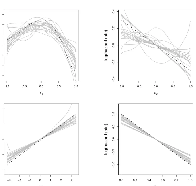
4.1.3 Simulation Results 2: Estimated Effects
Now, we look at the estimated effects and compare them with the real, specified effects. To keep the plots clear and readable we restricted the results to 20 models for each simulation scheme.
Simulation Scheme 1 In Figure 1, we see a selection of the estimated effects for the six effective covariates. Note that all function estimates and all true effects are centered such that their mean is equal to zero. This is required, as the “level” of the estimates can be altered: In each base-learner we have parameters for the intercept to allow the overall estimate to reach the right level. Hence, the intercept estimate of a base-learner is not connected with the effect of the corresponding covariate and thus the “level” of a base-learner is generally arbitrary. Actually we only want to compare the form of the estimated effects.
The effects ofx1 tox5 are estimated reasonable well. A selection of estimated effects can be found
in Figure 1 whereas the other effects are comparable to the depicted ones. The estimated effects of
x6 seem to have a larger bias but if we take the scale of the outcome (i.e., the log hazard rate) into
account we see that there is no big deviation.
Caused by the sparse data at the boundaries (note that we used a standard normal distribution to
simulatex3) the boundaries of the sine form ofx3are estimated quite poorly, whereas the middle part
is estimated quite sensible (not depicted here). For linear effects, the sparse tails do not pose such a
big problem as we see from x4. Only in some cases (23%, see Tab. 2 (left)) we have deviations from
linearity. The estimation in the center region is hardly effected and only slight deviations in the areas with less observations can be identified. Hence, linear effects seem to be hardly effected by sparse tails.
The estimated effects of the non-effective covariatesx7 tox15 (not depicted here) are more or less
oscillating around zero (if present). Again the normally distributed variables show a higher variation at the boundaries. Categorical variables, which are seldom selected (see Tab. 2 (left)), show the smallest deviations from “no effect”.
Simulation Scheme 2 Simulation scheme two has only effective covariates in the model formula. The focus is on the goodness of the estimation of time-varying effects and on the performance of the simultaneous model choice algorithm. In Section 4.1.2 we showed that CoxFlexBoost leads to a biased model choice in favor of time-varying effects. Note that for the plots in Figure 3 we did not take into account that the boosting procedure also selected time-varying effects for many covariates. Only the time-fixed effects are depicted except for the baseline hazard (see Fig. 2).
In the second simulation scheme, a dependent baseline hazard is added as well as a time-varying effect. The left panel of Figure 2 depicts the estimated log-baseline hazard over time in 20
models. Until time t ≈ 1 the curvature of the true effect is fairly well estimated. Thereafter, the
quality of the estimation rapidly decreases. This is due to the sparseness of the data as discussed above for normally distributed data. As it can be seen from the right graphic in Figure 2 the survival time has a sparse right tail which leads to unstable estimations as already pointed out by Gray [7].
Figure 3 shows a selection of the estimated effects, which are in some cases almost as good as in the first simulation but they all tend to be a bit more unstable. Especially the estimated effects of the
−1.0 −0.5 0.0 0.5 1.0 −0.8 −0.6 −0.4 −0.2 0.0 0.2 0.4 x1 log(hazard rate) −1.0 −0.5 0.0 0.5 1.0 −0.5 0.0 0.5 1.0 x2 log(hazard rate) −2 −1 0 1 2 −3 −2 −1 0 1 2 3 x4 log(hazard rate) 0.0 0.2 0.4 0.6 0.8 1.0 −0.2 −0.1 0.0 0.1 0.2 x6 log(hazard rate)
Figure 1: Simulation Scheme 1 – Estimation of covariate effects from 20 models (gray lines) and real effects (dashed lines). Effect estimates and real effects are centered.
(not depicted here) suffers from the same problem as the baseline hazard, i.e., the estimated function is very unstable in the sparse, right tail.
4.2 Application: Model for Surgical Patients
In the following section, we aim to build a model for patients with severe sepsis. Our retrospective analysis used data from a database, which was initiated in 1993 in the surgical intensive care unit, Department of Surgery, Klinikum Großhadern, Ludwig-Maximilians-Universit¨at M¨unchen, Germany, for local benchmarking and quality control. The documentation period started on March 1st, 1993, and lasted until February 28th, 2005. During this time, 5,079 patients (5,495 cases) were admitted to the intensive care unit. Baseline characteristics and detailed outcomes of that population were published recently [30, 31, 32]. A retrospective search of all eligible cases was conducted, where only cases that had to be treated because of severe sepsis were included. Patients likely to die of serious comorbid conditions (e.g., tumor progress) other than sepsis within the 90-day follow-up period were excluded
0.0 0.5 1.0 1.5 2.0 2.5 −2.0 −1.5 −1.0 −0.5 0.0 0.5 1.0 time log(hazard rate) 0.0 0.5 1.0 1.5 2.0 2.5 −2.0 −1.5 −1.0 −0.5 0.0 0.5 1.0 time log(hazard rate)
Figure 2: Simulation Scheme 2 – Left: Estimation of the baseline hazard from 20 models (gray lines) and real effect (dashed line). Right: Estimation of the baseline hazard for one model (gray line) and real effect (dashed line) together with rugs for the observed data. Offsets of effect estimates and real effects are set equal and the effects are centered.
from the analysis. Further inclusion criteria had to be met [2]. We obtained relevant covariates reflecting the state of the patient on admission day, and the 90-day survival time for 462 patients with severe sepsis. To build the model, we applied the proposed CoxFlexBoost algorithm to the data.
4.2.1 Application of CoxFlexBoost
To asses the stability of the variable selection and model choice process of component-wise boosting,
as implemented inCoxFlexBoost[28], we used 5 random subsamples, each with 362 observations, of
the severe sepsis data from Großhadern. The remaining 100 observations from each subsample were used to determine the stopping iteration.
Before entering the model, all continuous covariates except time were standardized on intervals
[xmaxxmin−xmin,xmaxxmax−xmin] = [xmaxxmin−xmin,xmaxxmin−xmin + 1], where xmin and xmax are the minimum and
maxi-mum of the respective covariate. This was done by dividing by the range of the covariate:
e
xi = x xi
max−xmin. (19)
Categorical covariates are dummy coded. Time enters the model unstandardized.
As we have realized in the simulation studies, it seems that boosting with model choice is unstable (w.r.t. the selected base-learners) and prefers time-varying base-learners.
The CoxFlexBoost algorithm is applied to the same data which has also been used in Hofner et
al.[3], where another model selection strategy called two-stage stepwise (TSS) procedure is proposed
for models with potentially time-varying effects. This makes it possible to directly compare the two methods. Thus, we want to look at the variable selection capabilities of both methods. The two-stage stepwise models were fitted with the software package BayesX (Vers. 1.51), which is freely available from http://www.stat.uni-muenchen.de/~bayesx[33].
In contrast to the two-stage stepwise procedure, CoxFlexBoost is not able to handle preset covari-ates. Such an approach could be included in the boosting framework, for example, by updating a set of mandatory covariates in every iteration (see, e.g., [34]). However, as this is not implemented in CoxFlexBoost so far, we did not use mandatory covariates but treated all covariates equal in the model
−1.0 −0.5 0.0 0.5 1.0 −0.8 −0.6 −0.4 −0.2 0.0 0.2 0.4 x1 log(hazard rate) −1.0 −0.5 0.0 0.5 1.0 −0.4 −0.2 0.0 0.2 0.4 x2 log(hazard rate) −3 −2 −1 0 1 2 3 −4 −2 0 2 4 x4 log(hazard rate) 0.0 0.2 0.4 0.6 0.8 1.0 −1.0 −0.5 0.0 0.5 1.0 x5 log(hazard rate)
Figure 3: Simulation Scheme 2 – Estimation of covariate effects from 20 models (gray lines) and real effects (dashed lines). Effect estimates and real effects are centered.
choice procedure. In contrast, in the application of the TSS procedure [3] six mandatory covariates were used. This potentially can affect the inclusion of further covariates heavily. Furthermore, we did not use the complete data set but just subsamples in order to estimate the stopping iterations based on the out-of-bag sample. This again may have an influence on the selection and estimation of base-learners.
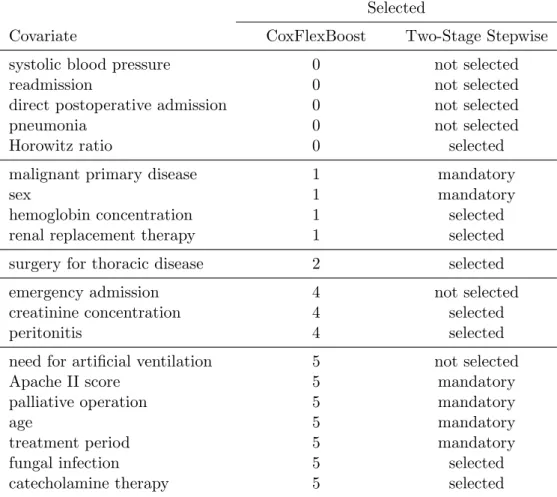
We extracted the selection frequencies for all variables in the CoxFlexBoost approach. A compar-ison with the model from the TSS approach can be found in Table 3.
We see that there is a fair range of agreement between CoxFlexBoost and the TSS procedure. To asses the disagreement, one needs to keep in mind that we used mandatory covariates in the TSS model, which perhaps would not have been added if a stopping criterion would have been applied. Both, “malignant primary disease” and “sex” were included in the starting model that consisted of the mandatory covariates despite they could not improve the conditional AIC. In the CoxFlexBoost model “renal replacement therapy” and “surgery for thoracic disease” were added only one or two times, respectively. In two-stage stepwise model they were added as the last two variables. This could
Selected
Covariate CoxFlexBoost Two-Stage Stepwise
systolic blood pressure 0 not selected
readmission 0 not selected
direct postoperative admission 0 not selected
pneumonia 0 not selected
Horowitz ratio 0 selected
malignant primary disease 1 mandatory
sex 1 mandatory
hemoglobin concentration 1 selected
renal replacement therapy 1 selected
surgery for thoracic disease 2 selected
emergency admission 4 not selected
creatinine concentration 4 selected
peritonitis 4 selected
need for artificial ventilation 5 not selected
Apache II score 5 mandatory
palliative operation 5 mandatory
age 5 mandatory
treatment period 5 mandatory
fungal infection 5 selected
catecholamine therapy 5 selected
Table 3: Selection of Covariates: Comparison of CoxFlexBoost and the two-stage stepwise procedure. For CoxFlexBoost the number of models in which the covariate was selected is given (max. 5). indicate that the inclusion of these covariates (in the TSS model) is at least arguable. “Horowitz ratio” and “hemoglobin concentration” were considered to be influential in the TSS model based on the conditional AIC. However, further inspection revealed that both effects only marginally depart from the zero-line, which would indicate that there is no effect at all. This is again in line with the results from CoxFlexBoost. “Need for artificial ventilation” and “emergency admission” were not included in the TSS model. CoxFlexBoost instead selected these variables as time-varying effects. As both variables have just a relatively small linear time-varying effect (see Fig. 4) these effects could be artifacts as well. Defining an inclusion rate of 2 or less negligible, only 10 out of 20 covariates can be regarded as influential covariates in the boosting model. The TSS procedure selected 14 covariates but 6 of these covariates were mandatory. Thus, a candidate model without a set of compulsory covariates could lead to a sparser final model. We can conclude that both the TSS procedure and CoxFlexBoost have a comparable strength for variable selection.
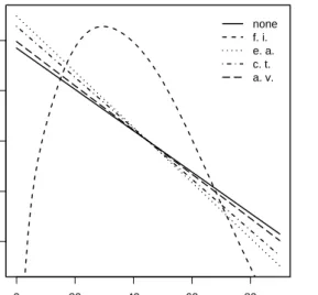
The resulting effects of the CoxFlexBoost models are hardly interpretable as many covariates are included with different modeling possibilities. They are added as smooth effects as well as time-varying
effects. In Figure 4 the time-varying effects of four categorical covariates are depicted for two of the
five estimated models. These two plots resemble the two archetypes of observed structures for the estimates of time-varying effects. Three models have the same structure as the model depicted in the left panel and the other two models have the same structure as depicted in the right plot. We only plotted the covariates that were selected in the majority of the five models. We could see that the log-baseline hazard is only selected in 3 out of the 5 models. Furthermore, it is remarkable that almost all time-varying effects were added as linear base-learners. Only observations in the subgroup
with “fungal infection” have approximately a quadratic log-hazard rate. The log-hazard in the other subgroups does not substantially differ from the log-baseline hazard of the model without an additional time-varying effect (Fig. 4, solid line), i.e., hardly any time-varying effect for these covariates can be observed. This is consistent in all five models.
0 20 40 60 80 −0.4 −0.2 0.0 0.2 0.4 time
log (hazard rate)
none f. i. e. a. c. t. a. v. 0 20 40 60 80 −0.4 −0.2 0.0 0.2 0.4 time
log (hazard rate)
none f. i. e. a. c. t. a. v.
Figure 4: CoxFlexBoost with model choice procedure for surgical patients data in 2 (out of 5) sub-samples: log(baseline hazard rate) in subgroups defined by “fungal infection” (f. i., present vs. absent), “emergency admission” (e. a.), “catecholamine therapy”(c. t.) and “artificial ventilation”(a. v.). All effects are centered.
Continuous covariates entered the model standardized. For some of the covariates, time-varying effects were also selected. Additional to the four categorical covariates with time-varying effect, six covariates were frequently added to the model: Three continuous covariates “Age”, “Apache II score” and “creatinine concentration” and three categorical covariates “palliative operation”, “peritonitis” (present vs. absent) and “treatment period” (before vs. after 2002). All three continuous covariates have a very high selection frequency for flexible time-varying effects. “Apache II score”, for example, was added as a strong nonlinear effect to the TSS model, whereas CoxFlexBoost estimated only a linear effect but added an additional time-varying effect. This increased flexibility of the combination of linear and time-varying effects cannot properly be depicted but it possibly obscures classical nonlinear
effects [18]. Looking at the effects for a given timet(we used median(ti)) ) all covariates have the same
directions of the effects as in the TSS model (cf. [3]): Effects that were estimated positive in the TSS model are also estimated positive in CoxFlexBoost, negative effect estimates were again estimated negative. However, all effects are smaller in CoxFlexBoost with respect to their norm. Note that this might not hold globally as we have additional time-varying effects that modify the given effects.
4.2.2 Comparison of Model Selection Strategies
Comparing the results of the application of the two-stage stepwise procedure (see [3]) and CoxFlex-Boost to the Großhadern data set of patients with severe sepsis, we can conclude that both approaches have advantages with regard to different aspects:
• The two-stage stepwise procedure includes only one modeling possibility from a given set of
different options, whereas CoxFlexBoost typically includes a variety of different modeling pos-sibilities for one covariate. Thus, in the boosting context, the ability to interpret the model
and the reliability of the model choice procedure suffer. A more sensible model choice scheme is needed in CoxFlexBoost without the selection bias in favor of time-varying effects.
• At the moment CoxFlexBoost cannot include mandatory covariates. However, such extensions
could be integrated in the algorithm. The two-stage stepwise procedure is easily extended in
such a way, as showed in Hofneret al. [3].
• With respect to the variable selection procedure, we can conclude that both approaches have
similar outcomes. In our application CoxFlexBoost tended to a sparser solution but this could be due to the starting model with mandatory covariates in the two-stage stepwise model.
• In settings with a large number of possible predictors, CoxFlexBoost is more convenient than
the two-stage stepwise procedure as it runs fully automatized. Moreover, CoxFlexBoost is able
to perform variable selection and model choice in data sets withnpand can even select more
covariates pthan we have got observations n.
Altogether, we see that none of the approaches is superior to the other. Decisions have to be based on the qualities of the algorithms in the given situation. Especially in high-dimensional settings with many possible predictors, boosting with its robustness against overfitting and the built in regularization is clearly the preferred method.
5 Summary and Outlook
In this paper, we derived boosting methods for flexible survival models with time-varying effects. For that purpose we used the full likelihood (and not the partial likelihood) as basis. This allows the estimation of the baseline hazard in the same framework by adding linear or smooth base-learners of time. We implemented a likelihood-based boosting approach as proposed in Tutz and Binder [20] to estimate the model. Component-wise boosting, which incorporates variable selection, has been shown to lead to appropriate models in terms of complexity. CoxFlexBoost and other likelihood-based boosting approaches maximize in each step the likelihood of one single base-learner with an offset consisting of the estimations of all previous iterations.
A major problem in flexible survival models are the many different modeling possibilities for each covariate. It is hard to decide if a covariate should enter the model as a linear term, smooth term or as time-varying effect or if the covariate is not required at all. Boosting offers the possibility to estimate the model with inherent model choice and variable selection. To incorporate the model choice procedure in component-wise boosting, we applied the effect decompositions for smooth effects
(9) and for time-varying effects (10) as proposed in Kneib et al. [12]. Furthermore, we assigned one
degree of freedom to the resulting centered flexible base-learners to make the modeling possibilities comparable with respect to their flexibility (cf. Sec. 3.1 and [12]). For the differentiation of linear and smooth effects, this provides good results. However, if one tries to distinguish between linear, smooth and time-varying effects at the same time, a selection bias in favor of time-varying base-learners is observed. A possible solution could be to standardize the observed survival time that enters the model as predictor variable. This will be subject to future research.
One possible alternative to the proposed model choice scheme in CoxFlexBoost could be to fit the
model in a similar fashion like that proposed in the MFPT approach by Sauerbrei et al. [8]. This
means, we fit a Cox-type model with time-constant but possibly smooth effects in a component-wise
boosting framework. To estimate the model one could make use of CoxFlexBoost[28] or apply the
mboost package with the CoxPH() family [29]. In a second step, one could try to addtime-varying effects only for the subsample of selected variables from above, where the derived model is used as starting model (i.e., as offset). Thus, base-learners for time-varying effects, for example, could be restricted to covariates without smooth effects leading to a model that is better interpretable and
perhaps overcomes the instability issues that we discussed above. Including time-varying effects for smooth effects would result in modeling an interaction of two functions: The function of the covariate and the function of time. This can be hardly ever estimated as we typically do not have enough data to fit the resulting interaction surface.
Another issue that arises frequently in medical applications is that some covariates are of clinically high importance and thus, should be included in the model by all means. These mandatory covariates can be incorporated in the boosting framework in such a way that these variables are updated in every boosting iteration [34]. This approach could also be included in CoxFlexBoost in future work.
Acknowledgments
The authors thank W. H. Hartl from the Department of Surgery, Klinikum Großhadern for the data set and stimulating problems and D. Inthorn and H. Schneeberger for initiation and maintenance of the database of the surgical intensive care unit. B. Hofner and T. Hothorn were supported by Deutsche Forschungsgemeinschaft, grant HO 3242/1-3.
References
[1] Cox DR. Regression models and life tables (with discussion). Journal of the Royal Statistical
Society. Series B 1972; 34:187–220.
[2] Moubarak P, Zilker S, Wolf H, Hofner B, Kneib T, K¨uchenhoff H, Jauch, K-W, Hartl WH. Activity-guided antithrombin III therapy in severe surgical sepsis: Efficacy and safety according
to a retrospective data analysis.Shock 2008; 30(6):634–641.
[3] Hofner B, Kneib T, Hartl W, K¨uchenhoff H. Model choice in Cox-type additive hazard regression
models with time-varying effects.Technical Report, Department of Statistics,
Ludwig-Maximilans-Universit¨at M¨unchen 2008. URL http://epub.ub.uni-muenchen.de/3232/.
[4] Zucker DM, Karr AF. Non-parametric survival analysis with time-dependent covariate effects: A
penalized likelihood approach. Annals of Statistics 1990; 18:329–352.
[5] Fahrmeir L, Kneib T, Lang S. Penalized structured additive regression: A Bayesian perspective. Statistica Sinica 2004;14:731–761.
[6] Hastie T, Tibshirani R. Varying-coefficient models.Journal of the Royal Statistical Society. Series
B 1993;55:757–796.
[7] Gray RJ. Flexible methods for analyzing survival data using splines, with application to breast
cancer prognosis.Journal of the American Statistical Association 1992; 87:942–951.
[8] Sauerbrei W, Royston P, Look M. A new proposal for multivariable modelling of time-varying
effects in survival data based on fractional polynomial time-transformation.Biometrical Journal
2007; 49:453–473.
[9] Abrahamowicz M, MacKenzie TA. Joint estimation of time-dependent and non-linear effects of
continuous covariates on survival. Statistics in Medicine 2007; 26:392–408.
[10] B¨uhlmann P, Yu B. Boosting with the L2 Loss: Regression and classification. Journal of the
American Statistical Association 2003; 98:324–339.
[11] B¨uhlmann P, Hothorn T. Boosting algorithms: Regularization, prediction and model fitting. Statistical Science 2007; 22:477–505.
[12] Kneib T, Hothorn T, Tutz G. Variable selection and model choice in geoadditive regression models. Biometrics 2008; (accepted).
[13] Royston P, Altman DG. Regression using fractional polynomials of continuous covariates:
Parsi-monious parametric modelling.Applied Statistics 1994; 43:429–453.
[14] Berger U, Sch¨afer J, Ulm K. Dynamic Cox modelling based on fractional polynomials:
Time-variations in gastric cancer prognosis. Statistics in Medicine 2003; 22:1163–1180.
[15] Perperoglou A, le Cessie S, van Houwelingen HC. Reduced-rank hazard regression for modelling
non-proportional hazards. Statistics in Medicine 2006; 25:2831–2845.
[16] Eilers PHC, Marx BD. Flexible smoothing with B-splines and penalties.Statistical Science 1996;
11:89–121.
[17] de Boor C. A Practical Guide to Splines. Springer, New York, 1978.
[18] Therneau TM, Grambsch PM.Modeling survival data: Extending the Cox model. Springer, New
York, 2000.
[19] Schmid M, Hothorn T. Boosting additive models using component-wise P-splines.Computational
Statistics & Data Analysis 2008; 53:298–311.
[20] Tutz G, Binder H. Generalized additive modelling with implicit variable selection by
likelihood-based boosting.Biometrics 2006;62:961–971.
[21] Friedman JH. Greedy function approximation: A gradient boosting machine. The Annals of
Statistics 2001; 29:1189–1232.
[22] Hurvich C, Simonoff J, Tsai C. Smoothing parameter selection in nonparametric regression using
an improved Akaike information criterion.Journal of the Royal Statistical Society, Series B 1998;
60:271–293.
[23] Hansen M, Yu B. Model selection and minimum description length principle. Journal of the
American Statistical Association 2001; 96:746–774.
[24] Hastie T. Comment: Boosting algorithms: Regularization, prediction and model fitting.Statistical
Science 2007; 22:513–515.
[25] Press WH, Teukolsky SA, Vetterling WT, Flannery B. Numerical Recipes in C: The Art of
Scientific Computing. Second Edition. Cambridge University Press, 1992.
[26] Bender R, Augustin T, Blettner M. Generating survival times to simulate Cox proportional
hazards models. Statistics in Medicine 2005; 24:1713–1723.
[27] R Development Core Team.R: A Language and Environment for Statistical Computing. R
Foun-dation for Statistical Computing, Vienna, Austria 2008. URLhttp://www.R-project.org, ISBN
3-900051-07-0.
[28] Hofner B. CoxFlexBoost: Boosting Flexible Cox Models (with Time-Varying Effects) 2008. URL
http://R-forge.R-project.org/projects/coxflexboost, R package version 0.5-0.
[29] Hothorn T, B¨uhlmann P, Kneib T, Schmid M, Hofner B. mboost: Model-Based Boosting 2008.
URLhttp://cran.R-project.org/web/packages/mboost, R package version 1.0-4.
[30] Hartl WH, Wolf H, Schneider CP, K¨uchenhoff H, Jauch KW. Secular trends in mortality
[31] R¨uttinger D, Wolf H, K¨uchenhoff H, Jauch KW, Hartl WH. Red cell transfusion: an essential
factor for patient prognosis in surgical critical illness? Shock 2007; 28:165–171.
[32] M¨uller MH, Moubarak P, Wolf H, K¨uchenhoff H, Jauch KW, Hartl WH. Independent
determi-nants of early death in critically ill surgical patients. Shock 2008; 30:11–16.
[33] Brezger A, Kneib T, Lang S. BayesX: Analysing Bayesian structured additive regression models. Journal of Statistical Software 2005;14(11):1–22. URLhttp://www.jstatsoft.org/v14/i11. [34] Binder H, Schumacher M. Allowing for mandatory covariates in boosting estimation of sparse