Environment. Technology. Resources, Rezekne, Latvia Proceedings of the 10th International Scientific and Practical Conference. Volume III, 22-28
Neurons vs Weights Pruning in Artificial
Neural Networks
Andrey Bondarenko, Arkady Borisov, Ludmila Aleksejeva
Riga Technical University
, Faculty of Computer Science and Information Technology,
Decision Support Systems Group.
Address: Mezha str. ¼ - 463, Riga, LV-1048, Latvia
Abstract. Artificial neural networks (ANN) are well known for their good classification abilities. Recent advances in
deep learning imposed second ANN renaissance. But neural networks possesses some problems like choosing hyper parameters such as neuron layers count and sizes which can greatly influence classification rate. Thus pruning techniques were developed that can reduce network sizes, increase its generalization abilities and overcome overfitting. Pruning approaches, in contrast to growing neural networks approach, assume that sufficiently large ANN is already trained and can be simplified with acceptable classification accuracy loss.
Current paper compares nodes vs weights pruning algorithms and gives experimental results for pruned networks accuracy rates versus their non-pruned counterparts. We conclude that nodes pruning is more preferable solution, with some sidenotes.
Keywords: artificial neural networks, generalization, overfitting, pruning.
I INTRODUCTION
Artificial neural networks has been successfully applied in many different areas to solve problems of classification and regression. ANN's, specifically multi-layer feed-forward artificial neural networks trained using error back-propagation give good results and recent advances in deep learning proved to give unprecedented classification accuracy [1]-[2]. Main problem with ANN's traiing is choosing hyper-parameters which can severely influence model performance. Choosing architecture with insufficient amount of neurons can give unsatisfying classification rates, while choosing too much neurons will badly influence training time and will cause overfitting. To overcome such problems two approaches exist: growing neural networks [3][4] and training excessively large network with subsequent pruning. In current paper we utilize second approach to overcome overfitting of trained ANN's, thus rise its generalization abilities as well as prepare previously trained artificial neural networks for rules extraction. We provide results of experiments with both nodes and weights pruning approaches.
Current paper is structured as follows: section two gives overview of pruning methods, section three describes used algorithm, section four presents results of experiments and sections five and six hold discussion and conclusion.
II PRUNINGMETHODSOVERVIEW Exist different approaches to ANN prunning. Both neurons themselves (thus all incomming and outgoing weights) and specific weights can be prunned. Paper [5] provides overview, we briefly present main ideas mentioned there along with other methods not listed in the source paper. We can divide all pruning algorithms into two main categories nodes/weights removal based on sensitivity analysis and penalty term based methods that utilize penalty term to remove 'unused' / least important weights. Some algorithms combine both approaches, while some cannot be easily added to one or the other family of methods. Sensitivity analysis relies on calculation of influence of specific node or weight.
Sensitivity analysis based methods
Sensitivity method from [6] by Mozer and Smolensy calculates error with unit removed and without it being removed, thus deleting least important units. Instead of calculating error directly they use derivative calculated during error back-propagation to approximate it. Segee and Carter in [7] have found that small variance in weights incoming into neuron is signaling that subject neuron can be safely removed.
Karnin in [8] describes method for weights pruning, which does not requires specific sensitivity calculation phase. All necessary data about weights updates are stored during training. This makes this approach unusable in case one wants to prune already trained
Andrey Bondarenko, et al./ Environment. Technology. Resources, (2015), Volume III, 22-28 ANN. Nevertheless such approach is perfectly usable
in case one have control over training of ANN. The main idea is sensitivity analysis of weights and their removal if they have too small sensitivity. Here is the
(1)
Where wf is specific weight value, 0 is its value after its pruning, E(wf) is error with given weight
enabled and E(0) is error when this weight is pruned. Finally Sij is sensitivity of weight between nodes i,j.
Instead of computing sensitivity value directly (which would lead to sensitivity estimation phase) authors propose to estimate it using sum of all changes of weight during training:
(2)
Rudy Setiono [9] Describes rather simple pruning algorithm which uses simple heuristics to find weights to be pruned. It assumes that one have ANN with single hidden layer (although approach can be generalized to multiple hidden layers), And afterwards removes input-hidden and hidden-output weights if their values are not satisfying specific constant. Actually there are two constants used, both of them should be set-up manually.
Rudy Setiono as well described rules extraction algorithm [10] called N2FPA which uses simple estimations of effect of removal of neurons in the network. Neurons are removed one by one. In case error worses significantly pruning stops. This is the method which was used and slightly modified in current paper.
Le Cun et.al in [11] describe method call Optimal Brain Damage (OBD) which measures “saliency” of a weight by estimating second derivative of the error with respect to the weight. They made couple of assumptions after which compute such derivatives during modified error back-propagation. One drawback of such method is necessity of storage of Hessian matrix. After one weight is pruned, retraining is done to find another weight to prune.
Optimal Brain Surgery from [12] (OBS) goes one step further in comparison to OBD, it utilizes inverse Hessian matrix to calculate optimal weight to be deleted, but at the same time it solves optimization
problem which as result gives remaining weights updates necessary to lower network error. Such approach allows simultaneous update of all remaining weights thus retraining is not required. OBS is one of the best methods for pruning. As well as OBD it should hold Hessian matrix thus requires additional memory.
Penalty based methods
Penalty term methods are utilizing weight decay / penalty term in one way or another to force neural network during its training get rid of unnecessary weights.
Chauvin [13] uses cost function with specific term which poses average energy expended by weights, as well there is a modification with additional magnitude of weights term which penalizes large weights and large amount of weights.
Weigend et. Al [14]-[16] minimizing specific cost function with additional term penalizing network complexity as a function of the weights magnitudes relative to the defined constant w0. Choosing such constant should be done via trials/errors.
Ji et.al [17] propose another penalty term based pruning approach based on modified error function which tries to minimize number of hidden nodes and weights magnitudes. The limitation of proposed method is that it assumes single hidden layer ANN with one input and out linear output node. Method assumes retraining after each removed weight.
Weight decay methods
Plaut et. Al [18] proposes simple cost function which decays weights. Cost function specifics tends to fact that algorithm favors nodes with lot of small weights in contrast to node with single large connection. Nowlan and Hinton [19] describe more complex cost function with penalty term which models the probability distributions of weights as mixture of Gaussians.
Interactive pruning
Sietsma and Dow [19] describe interactive method in which designer inspects network and marks nodes to be pruned. Algorithm provides several heuristics to determine candidates for removal. Authors have shown on training problems that their method is capable of finding relatively small networks with good accuracy in comparison to large trained networks which were not able to find solution.
f f f ij
w
w
E
w
E
S
0
)
0
(
)
(
^ Sij=−∑
n=0 N−1 ∂E ∂wij Δwij(n) wijf wijf−wijiAndrey Bondarenko, et al./ Environment. Technology. Resources, (2015), Volume III, 22-28
TABLE I
ERROR RATES WITH STANDARD DEVIATIONS.MEAN PRUNED NODES/WEIGHTS COUNTS.
Auto-pruning methods
Next discussed approach is auto-pruning method called lprune [20] by Lutz Prechelt. It proposes to prune at each step all weights not satisfying specific formula controlled by parameter lambda. Experiments showed that this parameter should be adaptive, algorithm to support dynamic adjustment is proposed. According to author proposed methods overcomes OBD and OBS in terms of accuracy and simplicity of pruned ANN
Another auto-pruning method [21] by William Finoff et. al utilizes modified cost function, does not requires full training of ANN and uses dynamic adjustment of penalty term. Similar to OBS this method performs dynamic topology adjustments.
Other methods
Kruchke [22] describes Local Bottlenecks method in which neurons “compete” with each other to survive. Magnitudes of vectors determine degree to which neuron participates in modeling target function, this is treated as neuron gain. In case gain is zero, neuron is not participating in classification task and can be removed. In case two neurons have parallel or anti-parallel weights vectors they are redundant and can be removed as well. Method utilizes specific parameter which should be tuned carefully.
Same author proposes another method called Distributed Bottlenecks [22][23] which puts constraints on weights rather than deletes them. This server as sort of dimensionality reduction. Such
approach makes weight vectors that are farther apart than average to become more farther from each other and vectors that are closer than average to become more closer. Again method uses special constant which should be chosen manually.
III PROPOSEDALGORITHM
We utilized algorithm described by Rudy Setiono in [10] (part of N2FPA rules extraction method.) In essence we are using nodes/weights pruning. We operate on trained ANN, on each pruning iteration we try to determine neuron or weight which needs to be removed. For all weights or neurons in input and hidden layers we calculate classification error for network operating without them. (This essentially means we are setting activations of pruned neurons to zero, or nullifying weights.) When neuron/weight, which upon removal gives network with smallest cost function is found it is removed. In our case this is neuron/weight which after removal gives network with smallest error classification rate. Afterwards network is retrained. If accuracy drops, remained the same or have risen over a small amount (we used tolerance equal to 2.5% - i.e. we are ok with error growth for this amount, then neuron/weight is really pruned. If error rises significantly candidate neuron/weight is left intact and new search for pruning candidate is initiated. In case error rises we are Retraining gives chances to get simpler network with high generalization and good classification rates, which can be observed looking into table 1.
MLP train avg. (std.dev) MLP test avg.. (std.dev Pruned Weights train avg.. (std.dev) Pruned Weights test avg.. (std.dev) Pruned Nodes train avg.. (std.dev) Pruned Nodes test avg.. (std.dev)
Pruned Weights (std.dev)
Pruned Counts (std.dev)
Haberman (10-fold X-validation) 25.99% (0.0098) 26.78% (0.0439) 24.39% (0.0102) 24.91% (0.0550) 24.98% (0.0101) 26.17% (0.0371) 54.9 (42.0) 23.8 (10.7) Ionosphere (10-fold X-validation) 10.83% (0.0013) 10.83% (0.0115) 4.21% (0.0117) 10.25% (0.0346) 4.55% (0.0116) 9.22% (0.0350) 34.1 (26.8) 34.3 (16.0) Monks-1 (train/test) 21.51% (0.0158) 32.74% (0.0138) 0.83% (0.0268) 1.81% (0.0566) 6.83% (0.0718) 13.22% (0.1201) 45.9 (17.3) 22.4 (16.3) Monks-2 (train/test) 38.46% (0.0194) 36.04% (0.0167) 12.47% (0.1795) 12.21% (0.1759) 11.26% (0.1751) 10.25% (0.1597) 16.8 (11.8) 20.1 (12.7) Monks-3 (train/test) 6.56% (0.0) 2.88% (0.0022) 5.16% (0.0182) 3.45% (0.0108) 3.33% (0.0068) 5.76% (0.0075) 32.4 (28.1) 29.3 (9.1) Parkinsons (10-fold X-validation) 24.58% (0.0023) 24.61% (0.0190) 14.83% (0.0307) 16.38% (0.0581) 14.30% (0.0154) 15.57% (0.0671) 10.5 (21.3) 8.3 (18.6) Pima (10-fold X-validation) 23.93% (0.0083) 24.56% (0.0436) 21.64% (0.0079) 23.74% (0.0398) 22.12% (0.0055) 23.05% (0.0322) 56.0 (34.3) 22.7 (3.3) WDBC (10-fold X-validation) 4.16% (0.0033) 4.33% (0.0251) 1.83% (0.0026) 2.63% (0.0238) 1.77% (0.0028) 2.93% (0.0218) 23.3 (9.2) 18.5 (11.0) WPBC (10-fold X-validation) 0% (0.0) 0% (0.0) 0% (0.0000) 0.17% (0.0091) 0% (0.0000) 0% (0.0000) 153.6 (140.6) 50.0 (0.0)
Andrey Bondarenko, et al./ Environment. Technology. Resources, (2015), Volume III, 22-28
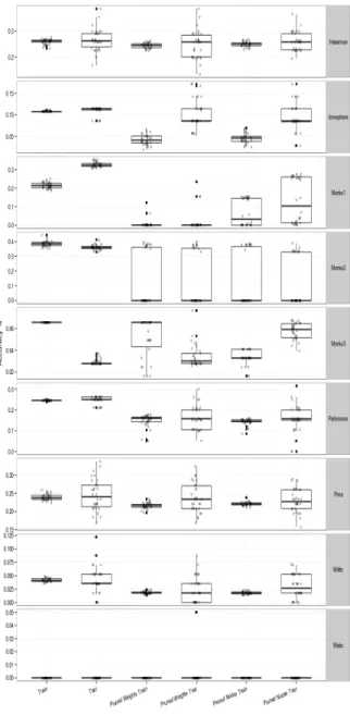
Fig. 1. Classification error.
This algorithm was described in our previous work [24]. Although in current papers we used a slightly modified version with two main changes. First of all in new version we have pruned not only hidden neurons but input layer as well – this basically worked as a feature selection. And secondly when algorithm encounters rise in error it saves ANN previous state, thus in case of several consecutive trials and failures to retrain network and get better accuracy (or at least not too bad – according to error tolerance) algorithm restores last known good ANN state (before significant rise of the error).
Below you can find pseudo code of weights pruning algorithm (with slight modifications in regards to algorithm published in [24]):
Inputs:
maxIter – determines maximum count of prunning iterations
maxPrunedNodes – maximum amount of nodes to be pruned
errorRiseTol - determines acceptable error rise
maxFallbacks - in case neurons are pruned and then reverted – how many times before we quit?
Program: iter = 1
while(iter<maxIter ||
prunedWeights<maxPrunedWeights)
for all not pruned weights in all layers if (lastWeightInLayer()) continue; removeWeight(n) cost = testNetwork() if (cost > largestKnownCost) largestKnownCost = cost indexOfPrunedWeight = getIndexOfPrunedWeight prunedWeights = prunedWeights + 1 end end S = saveNetworkState() retrainNetwork() classError = testNetwork() errRatio = classError/smallestClassError if (errRatio > 1 + errorRiseTol)
revert pruned weight
fallbacksCounter = fallbacksCounter + 1 prunedNodes = prunedNodes - 1
else
///leave pruned neuron as is fallbacksCounter = 0 end if (fallbacksCounter >= maxFallbacks) this = restoreNetworkState(S) break end iter = iter + 1 end
Here one can notice hyper-parameters listed in the beginning, maxIter -controls maximum possible amount of pruning iterations, maxPrunedNeurons – controls maximum amount of neurons to be pruned. We need both parameters as neurons after pruning can be restored, thus some iterations will not result in network pruning. Although they will leave network with weights adjusted during retraining. Apart from that two other hyper-parameters are: errorRiseTol –
Andrey Bondarenko, et al./ Environment. Technology. Resources, (2015), Volume III, 22-28 which controls maximum rise of error (we used
classification error) after removal of neuron which will not cause pruned neuron reversal/restore. Thus let's say in case error have risen for 5% in case of neuron removal in comparison to best/lowest known error rate and our parameter is 0.075 we will leave network intact, but if it is below 0.05 network will get back pruned neuron. Finally maxFallbacks controls how many attempts algorithm makes in pruning neurons and reverting them back consequently before termination. Thus if this parameter is equal to 10, then in case of ten subsequent iterations neuron is pruned, but then restored due to high rise in error algorithm terminates.
ANN itself is trained using Cross-entropy cost function equipped with penalty term (weights decay). Below is cost function:
(3) Where k – is the number of patterns,
l
ip = 0 or 1 is the target value for pattern xiat ouput unit p, p = 1,2,…,C.C is the number of output units/neurons.
S
ip is the output of the network at unit p:
(4)
Here to simplify things a bit we provide formulas for single hidden layered neural network, but in reality for our experiments we utilized two hidden layers. xi
is an n-dimensional input pattern, i=1,2,…,k. wm is an
n-dimensional vector of weights for the arcs connecting the input layer and the m-th hidden unit, m = 1,2,…,h. vm is a C-dimensional vector for the weight
connecting the m-th hidden unit and the output layer. The activation function is sigmoid function with domain (-1, +1):
(5)
Finally for all our weights we are applying weight decay factor 0.0001. This is quite simple approach in comparison to other described in theoretical part, but still it does the job. Cross-entropy was chosen as it is capable of dealing with problems of error derivative platoe better than standard round mean square error (RMSE) [25]. Apart from this we utilized Stochastic Gradient Descent batch training. Batch size was chosen to be 20.
IV EXPERIMENTS
In our experiments we have utilized three 10-fold cross-validation, but for some test-sets like monk's
train and test data are already provided thus there we utilized thirty runs to get averaged results. We decided to utilize two hidden layers neural networks so that some networks will be able to utilized this to their advantage, in case one of the layers is not needed we will be able to see this after pruning will be finished – such layers should have small amount of intact neurons in one of the layers. For our experiments we utilized well known UCI [26] data sets: Monks-1, Monks-2, Monks-3, Ionosphere, Haberman, Pima diabetes, WDBC, WPBC and Parkinsons.
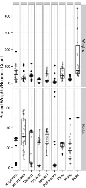
Fig. 2. Counts of pruned weights/nodes
Some of mentioned problems utilize only categorical variables - like monks. In such cases we have transformed input data into binary format thus instead of 5 inputs we used 17. In other cases the only transformation applied was rescaling of data into [-1, 1] region. Data sets are binary classification problems; we utilized two output neurons to represent solution of the network. Data sets themselves are pretty small
) log 1 )( 1 ( log ) , ( 1 1 k i C p i p i p i p i p S l S l v w F
m p m T i h m i px
w
v
S
1
ye
y
1
1
)
(
Andrey Bondarenko, et al./ Environment. Technology. Resources, (2015), Volume III, 22-28 ranging from about 150 to 500 entries. Table 1 holds
classification accuracy for all data sets. It contains average classification rate with standard deviation for both train and test cases along with 10 x-validation folds or runs for non-pruned and pruned neural networks. Last table column holds networks hidden layers structures before and after pruning.
For the pruning algorithm we used 0.025 as an errorRiseTol tolerance level, usually around 50 (depends on total amount of neurons, it should be around 60-70% of that) as maxIter iterations. MaxIter count should be larger than maximum amount of neurons to be pruned (which was always equal to neurons count in hidden layers minus 2 – we cannot prune all neurons from all layers.) In all cases we decided to utilize 2 layer hidden neuron networks (with error-backpropagation) trained using cross-entropy cost (error) function and stochastic gradient descent as learning algorithm. All cases were executed using 10-fold cross validation except monk’s data sets – they already are divided into training and testing sets
Figure 1 as well as Table 1 present classification errors for all 30 experiments across all datasets. One can note that all in all weights pruning when run on test data is giving classification accuracy almost equal to nodes pruning. Single exception is Monks-2 dataset, where weights pruning perform better. Now looking on figure 2 one can observe that counts of pruned nodes/weights greatly varies between runs. This suggests large amount of local minima. One way of dealing with this can be pre-training of ANN using DBN.
All in all training set classification graphs show decrease of train set classification error.
V DISCUSSION
As one can notice in many cases acquired ANN models are significantly smaller than initial networks. Exceptions are wdbc and parkinsons data sets where we can see ~50% drop in neurons counts. Both of them have rather complex structure thus require bigger models (in comparison to other data sets). Looking at weights pruning approach – almost always networks sizes are at least 70%-80% of the original size (with some exceptions). Looking at accuracy rates we can say there is a parity between weights and nodes pruning. Although in context of rules extraction neurons pruning is more preferable approach as it is producing smaller networks and it is less time consuming (there are much less neurons than weights in network). As we already noted algorithm have auto-stopping criteria allowing it to perform several trials before deciding to stop. Used algorithm assumes training of neural network with removed neuron/weight, while afterwards in case of unsatisfactory results removed neuron is returned back to the ANN. Diligent reader can note that there exists
several possibilities in regards to how and which neuron should be returned back into neural net. We used same neuron, but we have not explored possibilities of adding random neuron. As we already mentioned in case algorithm fails to get pruned network, it restores it’s last state – before it started to fail with removal of weight/node.
Another point to mention is interesting behavior of algorithm on Monks-2 dataset observing network errors in Figure 1 one can note that in half of all cases algorithm was able to get near zero error rate. At the same time weights pruning performed much better than nodes pruning at Monks-3 testing data set, which have 5% noise in training data.
VI CONCLUSIONS
In current paper we presented improved algorithm for pruning artificial neural networks via nodes/weights pruning along with experimental data (UCI classification data sets were used) showing that both types of pruning simplify network structure, but nodes pruning does better job. While weights pruning can give better results at cost of more complex ANN structure and higher computational time. Of course if some data set have complex structure – in such cases both approaches will end up with only slightly pruned neural network – but with better generalization value. When algorithm was applied to UCI datasets in many cases it produced much simpler ANN models with only a few neurons/or couple of dozens of weights while having slightly worse or in some cases better classification accuracy rates. Such 'simpler' models are faster to execute and are better candidates for knowledge extraction. Further research directions are exploration of other techniques for returning neuron back after retraining phase. Another area of future research can be dealing with local minima which causes early stopping during pruning. It is interesting to see causes of such early stopping – are they caused entirely by poorly trained ANN and can they be overcome or not.
VII REFERENCES
[1] A.-Krizhevsky, I. Sutskever, G. Hinton. “ImageNet
Classification with Deep Convolutional Neural Networks”,
Advances in Neural Information Processing Systems 25 (NIPS 2012), 2012.
[2] G. Hinton, L. Deong, D. Yu, G. Dahl and others, “Deep
Neural Networks for Accoustic Modelling in Speech
Recognition”. IEEE Signal Processing Magazine, November,
2012.
[3] X. Qiang, G. Cheng, Z. Wang, “An Overview of Some
Classical Growing Neural Networks and New Developments”,
IEEE, Education Technology and Computer (ICETC), 2nd International confernece Vol.3. 2010.
[4] V. Chaudhary, A.K. Ahlawat, R.S. Bhatia, “Growing Neural
Networks using Soft Competitive Learning”. International Journal of Computer Applications (0975-8887) Volume 21- No.3, May 2011.
Andrey Bondarenko, et al./ Environment. Technology. Resources, (2015), Volume III, 22-28
[5] R. Reed, “Pruning Algorithms – A Survey”, IEEE
Transactions on Neural Networks, Vol.4., No.5., September 1993.
[6] M. C. Mozer and P. Smolensky, "Skeletonization: A Techique
for Trimming the Fat From a Network via Relevance Assessment," in Advances in Neural Information Processing, pp. 107-115, (Denver 1988), 1989.
[7] B. E. Segee and M. J. Carter, "Fault Tolerance of Pruned
Multilayer Networks," in Proc. Int. Joint Conf. Neural
Networks, Vol. 2., (Seattle), pp.447-452, 1991.
[8] E. D. Karnin, "A Simple Procedure For Pruning
Back-Propagation Trained Neural Networks", IEEE Trans. Neural
Networks, Vol. 1., No. 2, pp.239-242, 1990.
[9] R. Setiono and H. Liu, "Understanding Neural Networks via
Rule Extraction," IJCAI, 1995.
[10] R. Setiono and W. H. Leow, "Pruned Neural Networks for
Regression" in PRICAI 2000 Topics in Artificial Intelligence,
Lecture Notes in Computer Science Vol. 1886, 2000, pp. 500-509.
[11] Y. Le Cun, J. S. Denker, and S. A. Solla, "Optimal Brain
Damage," in Advances in Neural Information Processing (2),
D.S. Touretzky Ed. (Denver 1989), 1990, pp. 598-605.
[12] B. Hassibi, D. G. Stork, G. J Wolf, "Optimal Brain Surgery
and General Network Pruning.”
[13] Y. Chauvin, “A Back-Propagation Algorithm With Optimal
Use of Hidden Units” Advances in Neural Information
Processing, (1) D.S. Touretzky ed. (Denver 1998), 1989, pp. 519-526.
[14] A. S. Weigend, D. E. Rumelhart, and B. A. Huberman,
"Back-Propagation, Weight Elimination and Time Series Prediction," in Proc. 1990 Connectionist Models Summer School, D. Touretzky, J Elman, T. Sejnowsky, and G. Hinton, Eds., 1990, pp. 105-116.
[15] A. S. Weigend, D. E. Rumelhart, and B. A. Huberman,
"Generalization by Weight-Elimination Applied to Currency
Exchange Rate Prediction," in Proc. Int. Joint Conf. Neural
Networks, vol. I, (Seattle), 1991, pp.837-841.
[16] A. S. Weigend, D. E. Rumelhart and B. A. Huberman,
"Generalization by Weight-Elimination With Application to
Forecasting," in Advances in Neural Information Processing
(3) R. Lippmann, J. Moody, and D. Touretzky, Eds., 1991, pp. 875-882.
[17] C. Ji, R. R. Snapp, and D. Psaltis, "Generalizing Smoothness
Constraints From Discreet Samples," Neural Computation,
Vol. 2, No. 2, 1990, pp.188-197.
[18] D. C. Plaut, S. J. Nowlan, and G E. Hinton, “Experiments on
Learning by Back Propagation,” Tech. Rep. CMU-CS-86-126,
Carnegie Mellon Univ., 1986.
[19] Sietsma, and R. J. F. Dow, "Neural Network Pruning – Why
and How" Proc. of the IEEE International Joint Conference
onNeural Netoworks, 1989, pp. 325-333.
[20] L. Prechelt, “Adaptive Parameter Prunning in Neural
Networks,” International Computer Science Institute, March. 1995.
[21] W. Finnoff, F. Hergert, and H. G. Zimmermann, “Improving
Model Selection by Nonconvergent Methods”, Elsiever
Neural Networks, Vol. 6, Issue 6, 1993, pp.771-783.
[22] J. K. Kruschke, “Creating Local and Distributed Bottlenecks
in Hidden Layers of Back-Propagation Networks,” in Proc.
1988 Connectionist Models Summer School, D. Touretzky, G. E. Hinton, and T. Sejnowsky, Eds., 1988, pp 120-126.
[23] J,. K. Kruschke, “Improving Generalization in
Back-Propagation Networks with Distributed Bottlenecks,” in Proc.
Int. Joint Conf. Neural Networks, Washington DC, Vol. 1, 1989, pp.443-447.
[24] A. Bondarenko, A. Borisov, “Neural Networks Generalization
and Simplification via Prunning”, Scientific Journal 2014 of Riga Technical University, 2014.
[25] P. Golik, P. Doetsch, and H. Ney, “Cross-Entropy vs. Squared
Error Training: a Theoretical and Experimental Comparison”, in Interspeech, pp. 1756-1760, Lyon, France, August 2013.
[26] K. Bache, M. Lichman, (2013), UCI Machine Learning
Repository [http://archive.ics.uci.edu/ml], Irvine, CA: University of California, School of Information and Computer Science (last accesed Sept 15, 2014).