Abhimanyu Gupta and Peter M. Robinson
Pseudo maximum likelihood estimation of
spatial autoregressive models with
increasing dimension
Article (Published version)
(Refereed)
Original citation:
Gupta, Abhimanyu and Robinson, Peter M. (2017)
Pseudo maximum likelihood
estimation of spatial autoregressive models with increasing dimension.
Journal of Econometrics
. ISSN
0304-4076
DOI:
10.1016/j.jeconom.2017.05.019
Reuse of this item is permitted through licensing under the Creative Commons:
© 2017 The Authors
CC BY-NC-ND
This version available at:
http://eprints.lse.ac.uk/84085/
Available in LSE Research Online: August 2017
LSE has developed LSE Research Online so that users may access research output of the School.
Copyright © and Moral Rights for the papers on this site are retained by the individual authors and/or
other copyright owners. You may freely distribute the URL (
http://eprints.lse.ac.uk
) of the LSE
Accepted Manuscript
Pseudo maximum likelihood estimation of spatial autoregressive models with increasing dimension
Abhimanyu Gupta, Peter M. Robinson
PII: S0304-4076(17)30145-8
DOI: http://dx.doi.org/10.1016/j.jeconom.2017.05.019
Reference: ECONOM 4404
To appear in: Journal of Econometrics Received date : 23 October 2015
Revised date : 26 April 2017 Accepted date : 30 May 2017
Please cite this article as: Gupta A., Robinson P.M., Pseudo maximum likelihood estimation of spatial autoregressive models with increasing dimension.Journal of Econometrics(2017), http://dx.doi.org/10.1016/j.jeconom.2017.05.019
This is a PDF file of an unedited manuscript that has been accepted for publication. As a service to our customers we are providing this early version of the manuscript. The manuscript will undergo copyediting, typesetting, and review of the resulting proof before it is published in its final form. Please note that during the production process errors may be discovered which could affect the content, and all legal disclaimers that apply to the journal pertain.
Pseudo Maximum Likelihood Estimation of Spatial
Autoregressive Models with Increasing Dimension
Abhimanyu Gupta
∗Department of Economics
University of Essex, UK
Peter M. Robinson
†Department of Economics
London School of Economics, UK
August 17, 2017
Abstract
Pseudo maximum likelihood estimates are developed for higher-order spatial autoregres-sive models with increasingly many parameters, including models with spatial lags in the dependent variables both with and without a linear or nonlinear regression component, and regression models with spatial autoregressive disturbances. Consistency and asymptotic normality of the estimates are established. Monte Carlo experiments examine finite-sample behaviour.
JEL classifications: C21, C31, C36
Keywords: Spatial autoregression; increasingly many parameters; consistency; asymptotic normality; pseudo Gaussian maximum likelihood; finite sample performance
∗Email: [email protected].
†Corresponding author. Email: [email protected], Telephone: +44-20-7955-7516Fax:
1
Introduction
Spatial autoregressive (SAR) models, introduced by Cliff and Ord (1973), can describe spatial dependence parsimoniously even when data are irregularly-spaced or when economic (not neces-sarily geographic) distances between units are known, and information on locations is unavailable. They have been widely used in modelling economic and geographic data. The first-order SAR model, which involves a single weight matrix, consisting of (inverse) distances, and a single cor-relation parameter, has been the focus of much research. Greater flexibility, at the cost of less parsimony, is afforded by higher-order SAR models, which incorporate two or more weight ma-trices and corresponding parameters. These have been studied in both theoretical and applied research. Brandsma and Ketellapper (1979) introduced a second-order model, and discussed its estimation. Blommestein (1983, 1985), Blommestein and Koper (1992, 1997), Anselin and Smirnov (1996), LeSage and Pace (2011), Elhorst, Lacombe and Piras (2012) and others ex-plored various issues in the specification and estimation of higher order SAR models, the latter two references listing a number of others. A recent purely empirical study is in Kolympiris, Kalaitzandonakes, and Miller (2011). A book length exposition can be found in Anselin (1988). In the present paper we investigate large sample statistical inference on higher order SAR models, in which the number of parameters is allowed to increase slowly with sample size, denoted
n, a type of setting previously studied by Gupta and Robinson (2015). From this perspective we find it convenient to consider four specifications that have somewhat different theoretical as well as practical implications. For ann×1 vectoryn of observations and an integerpn≥1,possibly
regarded as increasing as n increases, let Win, i = 1, . . . , pn, be n×n known weight matrices
whose elements are inverse economic distances, let λ0n = (λ01, . . . , λ0pn)
0, the prime denoting
transposition, be a vector of unknown parameters, and letube ann×1 vector of independent, zero-mean, homoscedastic unobservable random variables. The basic pnth-order SAR model,
denoted SAR(pn),is yn= pn X i=1 λ0iWinyn+u. (1.1)
Letlnbe an×1 vector of ones and letτ0be an unknown scalar. The SAR(pn) with intercept is
yn= pn
X
i=1
λ0iWinyn+τ0ln+u. (1.2)
For given integerskn≥1 (possibly regarded as increasing withn) and fixedq≥1 letβ0n be an
unknownkn×1 vector, letδ0be a known or unknownq×1 vector and letXn(δ0) be ann×kn
matrix of functions of δ0 and of explanatory variables, with reference to the latter suppressed.
The SAR(pn) with regressors is
yn= pn
X
i=1
Finally, for ann×1 vector vn of unobservable random variables, the regression with SAR(pn) errors is yn =Xn(δ0)β0n+vn, vn= pn X i=1 λ0iWinvn+u. (1.4)
These models correspond to versions ofpnth-order autoregressive time series models, where
com-peting approaches to introducing both autocorrelation and explanatory variables are mirrored by (1.3) and (1.4).
When τ0 is known (1.2) nests (1.1) (which is sometimes referred to as ‘pure SAR’), while
(1.2) is nested in both (1.3) and (1.4) when Xn(δ0) contains a subvector ln, although
estima-tion methods differ. Indeed (1.1) and (1.2) are not consistently estimable by least squares or instrumental variables, unlike (1.3) and (1.4). In most spatial autoregression literature, SAR(1) versions of these models have been studied, and previous higher-order SAR literature has almost exclusively assumed that pn and kn are fixed. In the the bulk of the literature on (1.3) and
(1.4) the regression component is linear, formally covered by regardingδ0 as known. However,
(1.3) and (1.4) allow for nonlinear regression, which features widely in statistics (cf. eg Jennrich (1969)) and econometrics but apparently not in the SAR literature, even though Xu and Lee (2015) have studied a SAR model with a nonlinear transformation of the dependent variable. For example, the elements of Xn(δ0) may be parametric Box-Cox, arcsinh or other nonlinear
transformations of basic explanatory variables. The separation ofβ0n from δ0 follows much of
the nonlinear regression literature in expressing the likely presence of an unknown scaling vector. Then-subscripting inXn(δ0) allows it to depend on spatial lags of explanatory variables, which
entail weight matrices. The model (1.4) may be included in (1.3) by replacing Xn(δ0) by a
function of both δ0 and λ0n, but (1.4) is of sufficient practical importance to warrant separate
consideration.
Interest centres on statistical inference on λ0n, β0n and, when it is unknown, δ0. Consider
what is known or anticipated from the literature that regards pn and kn as fixed. In (1.1)
and (1.2), despite the linearity in parameters, least squares estimates are well known to be inconsistent, for typicalWin,which differ from the lower triangular ones which deliver consistency
in the autoregressive time series models formally covered; however, for (1.1) Kelejian and Prucha (1999) established consistency of a generalized method of moments estimate. For the same reason consistency of least squares estimates of all parameters in (1.3) is problematic, though from Lee (2002) (who assumed pn = 1 and linear regression) we may expect consistency to be
achieved under certain asymptotic conditions on the Win. Under milder such conditions, again
when the regression is linear, use of instrumental variables, when available, can produce closed form consistent estimates in (1.3), see eg Kelejian and Prucha (1998); for nonlinear regression one expects to be able to extend, eg, Amemiya (1974). As under many other relaxations of Gauss-Markov conditions, least squares estimates of β0n in the first equation of (1.4) (or nonlinear
least squares estimates ofβ0n andδ0) are expected to be consistent, though those ofλ0n based
one expects them to satisfy a central limit theorem under additional conditions. The models (1.1)-(1.4) are somewhat idealised, some of the literature considering ones that are more general. In ‘SARAR’ versions of (1.1), (1.2) or (1.3), u is replaced by vn, defined as in (1.4) but with
pn possibly replaced by some other order rn, say. However after transformation they are still
essentially covered by (1.1)-(1.3), albeit offering more parsimony, having SAR order pnrn with
coefficients depending on onlypn+rnunknowns. In a SARAR version of (1.3), Lee and Liu (2010)
established asymptotic theory for generalized method of moments estimates, as did Badinger and Egger (2011, 2013), allowing respectively for error heteroscedasticity and panel structure. Spatial ARMA models are not covered in (1.1)-(1.4); in this setting Huang (1984) and Anselin (2001) respectively discussed maximum likelihood estimation and developed Lagrange multiplier tests to determine model order.
A single type of estimate which can be expected to deliver consistency, and asymptotic normality, in (1.1)-(1.4), and without recourse to instrumental variables, is the Gaussian pseudo-maximum likelihood estimate (PMLE). This maximizes what would be the likelihood were u
Gaussian, and as well as enjoying the classical asymptotic properties of maximum likelihood, is consistent and asymptotically normal under more general conditions onu,though in some settings the limiting covariance matrix can be affected. Brandsma and Ketellapper (1979) discussed Gaussian maximum likelihood estimation in the SAR(2) version of (1.1), describing, without rigorous proofs, asymptotic statistical properties, see also Huang (1984). These properties were established for the PMLE by Lee (2004) in case of SAR(1) versions of (1.1)-(1.3) with linear regression in the latter model. The PMLE is asymptotically efficient whenuis Gaussian, though otherwise more efficient estimates have been justified in fixed parameter dimension SAR models, see Lee and Liu (2010) and Robinson (2010). Note that our allowance for nonlinear regression does not greatly impact on methods and theory for the PMLE, which is in any case only implicitly defined. One well-known aspect of the PMLE is the need to invert an n×n matrix in the estimation. On the other hand, a general defence of the PMLE is its asymptotic efficiency properties in the Gaussian case, the fact that consistency and the same limit distribution holds under more general conditions than Gaussianity, and the relatively simple and easy-to-compute form of the limiting covariance matrix estimate following the point estimation.
In practice the specification of pn, and of kn, may be influenced by the amount of data n
available, as is the case with other multiparameter statistical models. A larger data set affords the possibility of achieving reasonably precise inference on a richer model, which may reflect a degree of model uncertainty. Correspondingly, in a number of other multiparameter models, asymptotic statistical theory has been developed with the number of parameters increasing slowly with sample size, cf. Huber (1973), Berk (1974), Sargan (1975), Robinson (1979), Portnoy (1984, 1985), Robinson (2003). Gupta and Robinson (2015) have argued that regarding pn
as increasing with n is natural in SAR models with some kinds of weight matrix, and have established asymptotic theory for least squares and instrumental variables estimates of (1.3) in the linear regression case. A popular alternative approach to models with a large number of
parameters is to apply the LASSO, or a similar estimate based on a penalized objective function. This method is especially useful in cases wherepn+kn≥n.
The present paper establishes consistency and asymptotic normality for the PMLE in the models (1.1)-(1.4) with pn and kn allowed to increase slowly with n. Asymptotic theory for
implicitly-defined extremum estimates, requiring an initial consistency proof, is unusual in the literature on increasing parameter dimension with sample size, especially so when combined with nonlinear regression. Our proof of consistency of the PMLE is rather delicate, in particular where both numerator and denominator terms increase with kn (see (A.8) in the appendix), while we
also need the volume of the admissible autoregressive parameter space to remain bounded aspn
diverges. Our results lead to rules of statistical inference which are also valid whenpn and kn
are regarded as fixed, and to some extent provide a novel contribution in this setting also. In particular we know of no asymptotic theory for the PMLE in the models (1.1)-(1.4) with fixed
pn >1 andkn.We keep the dimensionqofδ0 fixed as otherwise the regression would effectively
be nonparametric.
The following section covers models (1.1) and (1.2), with (1.3) and (1.4) covered in Sections 3 and 4, respectively. Section 5 contains a Monte Carlo study of finite sample performance. Proofs are included in two Appendices and an additional online supplementary appendix.
2
SAR with and without intercept
We can rewrite (1.1) as
Snyn =u (2.1)
whereSn=In−Pip=1n λ0iWin. The notationSnfollows a convention we adopt for evaluation of
objects at true parameters: A(α0)≡Afor any matrix, vector or scalarAand any true parameter α0. In the sequel we suppress reference tonfor individual parameters to simplify notation. We
now introduce some basic assumptions.
Assumption 1. u= (u1, . . . , un)0 has independently distributed elements with zero mean, finite
variance σ2
0 and finite third and fourth momentsµ3 and µ4 respectively.
Assumption 2. For i = 1, . . . , pn, the diagonal elements of each Win are zero and the
off-diagonal elements ofWinare uniformlyO h−n1
, wherehnis a positive sequence which is bounded
away from zero and which may be bounded or divergent, withn/hn → ∞asn→ ∞in the latter
case.
It is possible to employ different hin for each of the Win, some bounded and some divergent.
However we maintain Assumption 2 for notational simplicity. For any rectangular matrixA, we definekAk=ζ(A0A)
1 2
, where ¯ζ(B) (respectivelyζ(B)) is the largest (smallest) eigenvalue of a square, symmetric matrixB.
Definition Fori= 1, . . . , pn, Winare said to have ‘single nonzero diagonal block’ structure if,
for some set of mi×mi matrices Vinsuch that Pip=1n mi =n, Winhas Vin as theith diagonal
block and zeros elsewhere.
Letc,C denote throughout generic positive constants, arbitrarily small and large, respectively.
Assumption 3. Sn is non-singular and
S−1 n + max i=1,...,pnk Wink ≤C, (2.2)
for all sufficiently large n.
The first part of this assumption ensures that (2.1) can be solved for yn, asymptotically. The
restriction onS−1
n
limits spatial correlation because the covariance matrix ofynisσ02Sn−1Sn−10,
while the restrictions on the kWink are satisfied if, for each i, the elements of Win decline fast
enough withn. A sufficient condition for the non-singularity ofSn is
pn X i=1 λ0iWin <1. (2.3)
Depending on the structure ofWin more primitive sufficient conditions can be given for (2.3).
Denote by λ = (λ1, . . . , λpn)
0 and σ2 any admissible values of λ
0n and σ02 and let kak1 =
Ps
i=1|ai| for any s-dimensional vector a. In the ‘single nonzero diagonal block’ case we have kPpn
i=1λ0iWink ≤ maxi=1,...,pn(|λ0i| kVink), in which case one could take the parameter space Λn forλto be such that
max
i=1,...,pn|
λi|<1, (2.4)
and take normalizedVinsuch that kVink= 1. For more generalWinwe havekPpi=1n λ0iWink ≤
maxi=1,...,pnkWink
Ppn
i=1|λ0i|, and then we may choose Λn such that
kλk1<1, (2.5)
and normalize the Win such that kWink ≡ 1. In any case, for the identification of the λi
some normalization of theWin is necessary, so this operation is essentially costless. A similar
discussion applies after Assumption 12 below, with row-sum norm used instead. Define the negative Gaussian log-likelihood function as
log (2πσ2)−2n−1log|Sn(λ)|+σ2n−1y0nSn(λ)Sn(λ)yn, (2.6)
for nonsingularSn(λ) =In−Pip=1n λiWin. For givenλ, (2.6) is minimised with respect toσ2by
¯
Define the PMLEs ofλ0n,σ20 as ˆλn= arg minλ∈ΛnQn(λ),ˆσ 2 n≡σ¯2n ˆ λn respectively, where Qn(λ) = log ¯σn2(λ) +n−1log Sn−1(λ)Sn−10(λ) , (2.8) with Λn satisfying
Assumption 4. Λn is a subset ofRpn such that, for some fixedε∈(0,1),−ε≤λi≤1−ε, for
i = 1, . . . , pn when the Win have ‘single nonzero diagonal block’ structure and kλk1 ≤1−ε if
not.
Assumption 4 reflects the necessity in our proof that the volume of Λn remain bounded as
n→ ∞, and the likelihood that theλ0i are non-negative, but could be replaced by others. The
construction of a compact parameter space requires some care when dimension can increase. The usual Cartesian product of closed and bounded intervals that forms a compact parameter space in the fixed dimension setting will not, in general, yield a region with bounded volume when dimension increases. The Associate Editor handling our paper has pointed out that by analogy with results shown in other settings (see eg P¨otscher and Prucha (1997) pp. 29-31 and references therein, and Kuersteiner and Prucha (2015)), the compactness requirement of Assumption 4 might be relaxed and the arbitrary choice ofεavoided by, more naturally, choosing Λnas (2.4) in
the ‘single nonzero diagonal block’ case, and as (2.5) otherwise. The only drawback to optimizing over an open set would appear to be that ˆλn might sometimes not exist. On the other hand
with compact Λn, if ˆλn falls on its boundary it is likely that shrinkingεwould change ˆλn.This
may suggest thatnis too small for asymptotics to be relevant, and/or the parameter space has been chosen too small or the model is misspecified. Typically there will be no option to collect further data, while employing an alternative method of estimation in the hope that the outcome will lie within the boundary seems an over-reaction, especially as one can chooseεso small that shrinking it would not affect ˆλnto any desired number of decimal places, or indeed make any
statistically significant difference. Our use ofkλk1≤1−ε,or indeed (2.5), in non-‘single nonzero
diagonal block’ cases is nevertheless still unsatisfactory because, with the restriction on theWin,
it is a crude sufficient condition for (2.3), compared to the precise conditions for stationarity of autoregressive time series in terms of the locations of zeros of the autoregressive polynomial. Further work to relax Assumption 4 in our increasing parameter dimension setting would be desirable.
Note that though we treat theWinas known, in reality the scaling of distances is arbitrary
and different scalings are used in the literature. Some scaling, such askWink= 1, is necessary
in order to identify the λ0i and correspondingly specify a suitable Λn. We could replace each
WinbycWinforc∈(0,∞) and Λn byc−1Λn, but for identification we must choose one scaling
and one parameter space.
Denote
σn2(λ) =n−1σ20tr Sn−10Sn0 (λ)Sn(λ)Sn−1
. (2.9)
Assumption 6. Forλ∈Λn and all sufficiently largen,c≤σ2n(λ)≤C.
σ2
n(λ) is nonnegative by inspection and finite by Assumptions 3 and 4. For a generic matrixA
definekAkF ={tr(A0A)}12 and introduce
Assumption 7. For any η >0,
lim n→∞λ∈Ninfnλ(η) n−1kTn(λ)k2F/|Tn(λ)|2/n>1, (2.10) whereTn(λ) =Sn(λ)Sn−1,N λ n (η) = Λn\ Nnλ(η), Nnλ(η) ={λ:kλ−λ0nk< η} ∩Λn.
The ratio in (2.10) is guaranteed ≥ 1 due to the inequality between arithmetic and geometric means. Assumption 7 is an identification condition related to the uniqueness of the covariance matrix ofyn, introduced in Delgado and Robinson (2015) who discussed it and compared it to
the identification condition employed by Lee (2004) in his asymptotic theory.
Theorem 2.1. Let (1.1) and Assumptions 1-7 hold, andpn be allowed to diverge as n→ ∞.
Then ˆλn−λ0n −→p 0, asn→ ∞.
Theorem 2.2. Let (1.1) and Assumptions 1-7 hold, and pn be allowed to diverge as n → ∞
such thatp2n/nhn→0. Thenσˆn2−σ20=op(1), asn→ ∞.
Multimodality can be a potential problem with implicitly defined extremum estimates, see eg Warnes and Ripley (1987) in a rather different spatial context. It is plausible that the likelihood of it could increase with increasingpn or decreasingn, or perhaps with ‘increasing nonlinearity’.
However on the one hand one could get multimodality when p= 1, and on the other, normal multiple linear regression is always unimodal if kn < n. Certainly the smaller the gap between
nand pn the flatter we might expect the objective function to be, but this a local rather than
global issue. The problem does not necessarily go away with large n, as even if the objective function is asymptotically uniquely optimised asymptotic sub-optimal modes are not ruled out. For p = 1 Hillier and Martellosio (2013) are able to establish unimodality if W1n has real
eigenvalues (amongst other conditions), although their approach relies on an explicit analysis of the second derivative of the likelihood function and seems difficult to extend whenp >1. One way to mitigate the problem is by searching over a sufficiently fine grid before any iteration, though the largerpn is the more expensive this is.
To establish asymptotic normality, we denote byHn λ, σ2the second derivative matrix of
(2.6) and define it in (A.18) in Appendix A. WritingP1n(λ), P2n(λ) for the pn×pn matrices
WinS−n1(λ) fori= 1, . . . , pn, we deduce (details in Appendix A) that
Ξn=E(Hn) = 2n−1(P1n+P2n). (2.11)
WriteFn for then×pn matrix with (i, j)-th elementcii,jn, where cpq,in is the (p, q)-th element
of Gin+G0in, and define Ωn = µ4−3σ04
σ−04n−1F0
nFn. The covariance matrix of the first
derivative of (2.6) isn−1(2Ξ
n+ Ωn). The following assumption is standard:
Assumption 8. λ0n is in the interior of Λn, for all sufficiently large n.
Ifhn diverges withn, we need to account for the correct normalisation that will yield a central
limit theorem as follows:
Assumption 9. hn→ ∞asn→ ∞. lim
n→∞ζ(hnΞn)<∞ andnlim→∞
ζ(hnΞn)>0.
Assumption 10. hn is bounded asn→ ∞. lim n→∞ζ Ξ −1 n ΩnΞ−n1 <∞, lim n→∞ζ 2Ξ −1 n + Ξ−n1ΩnΞ−n1 >0 and lim n→∞ζ(Ξn)>0.
The rank conditions here strongly restrict theWinin higher-order SAR models, even with fixed
pn. Such problems are transparently avoided with weight matrices having ‘single nonzero
di-agonal block’ structure. Blommestein (1985) discusses the possibility of ‘circularity’ when Win
represent orders of contiguity, causing rank condition failure. By way of an illustration, W1n
could assign 1 to an element if the relevant units share a common boundary,W2n could assign 1
to an element if the relevant units do not share a boundary with each other but have a common neighbour, and so on. In this case, there is a risk of high-orderWin ‘circling’ back toW1n.
Assumption 11. For someχ >0,E|ui|4+χ≤C,i= 1, . . . , n.
For any s×q matrix A = [aij] define kAkR = maxi=1,...,sPqj=1|aij|, the maximum absolute
row-sum norm.
Assumption 12. Sn is non-singular and
S−1 n R+ S0−1 n R+ maxi=1,...,pn(kWinkR+kW 0 inkR)≤C, (2.12)
for all sufficiently large n.
This strengthens Assumption 3 due to the inequalitykAk2≤ kAkRkA0kR.
Denote throughout by Ψn a matrix of constants with full and fixed row rank, and columns
equal in number to the parameters for which a central limit theorem is being established. Our next theorem covers the unboundedhncase, establishing asymptotic normality of a fixed number
Theorem 2.3. Let (1.1) and Assumptions 1, 2, 4, 6-9, 11 and 12 hold, hn → ∞asn→ ∞,pn
be allowed to diverge as n→ ∞such that p5 n nhn +pn hn +p 4 nh2n n + p2+ 8 χ n h 1+4 χ n n →0 as n→ ∞. (2.13) Then n12 h12 np 1 2 n Ψn ˆ λn−λ0n d −→N(0,∆1), as n→ ∞, where∆1= 2 limn→∞p−n1Ψn(hnΞn)−1Ψ0n.
First, note that χ > 4 implies that the last term on the LHS of (2.13) is dominated by the third one. If GjnGin = 0 and Gjn0 Gin = 0 for i 6= j, as with ‘single nonzero
diag-onal block’ weight matrices, then any finite-dimensidiag-onal subset of estimates will be asymp-totically distributed as independent normal random variables with mean zero and variances
limn→∞(hn/n)tr G2in+G0inGin −
1
. If pn is fixed then the restrictions on pn in (2.13)
are redundant. In this case the same proof, considering a single linear combination, implies
n12/h 1 2 n λˆn−λ0 d →N0,2 limn→∞(hnΞn)−1
, by the Cramer-Wold device. We may derive similar results for fixed parameter spaces from the subsequent central limit theorems in this section. The following theorem takeshn to be bounded, complementing Theorem 2.3.
Theorem 2.4. Let (1.1) and Assumptions 1, 2, 4, 6-8, 10-12 hold, andpn be allowed to diverge
asn→ ∞ such that p5 n n + p2+ 8 χ n n →0, asn→ ∞. (2.14) Then n12 p 1 2 n Ψn ˆ λn−λ0n d −→N(0,∆2), asn→ ∞, where∆2= limn→∞p−n1Ψn 2Ξn−1+ Ξ−n1ΩnΞ−n1 Ψ0 n.
The parameter growth restrictions may be simplified if moment conditions are strengthened. For instance when χ ≥8/3 in Assumption 11, (2.14) only requires p5
n/n →0. Covariance matrix
estimation for Theorems 2.3 and 2.4 can be based onHn λ, σ2n
and Ωn λ, σ2n evaluated at ˆλn, ˆ σ2
n and empirical moments.
We now turn from model (1.1) to the slightly more general (1.2). For any admissibleλ,τ and
σ2 and nonsingular S
n(λ) the negative Gaussian pseudo log-likelihood function is log (2πσ2)−
2n−1log|S
n(λ)|+ nσ2−
1
kSn(λ)yn−lnτk2,which for givenλis minimised with respect toτ
andσ2by ¯τ
n(λ) =n−1ln0Sn(λ)ynand ¯σn2(λ) =n−1yn0Sn0 (λ)MlnSn(λ)yn, where we writeMA=
In−A(A0A)−1A0for anyn×smatrixAof ranks, withIndenoting then×nidentity matrix. The
PMLE ofλ0is ˆλn= arg minλ∈ΛnQn(λ),whereQn(λ) = log ¯σ 2 n(λ) +n−1log S−1 n (λ)Sn−10(λ) ,
and the PMLEs ofτ0 and σ20 are ˆτn = ¯τn
ˆ λn and ˆσ2 n = ¯σn2 ˆ λn
respectively. The first and second derivatives evaluated at λ00n, τ0, σ02
are writtenξI
derivatives with respect toτ, and explicit expressions can be obtained by takingXn =lnin (1.3).
The covariance matrix of the first derivative of the likelihood function isn−1 2ΞI n+ ΩIn , with ΞI n=E HnI .
A feature of this model noted by Lee (2004) is potential multicollinearity. For example, if theWin are row-normalised (with non-negative elements) thenWinln =ln, so thatGinlnτ0 = τ0ln(1−Ppi=1n λ0i)−1for eachi. It follows thatMlnGinlnτ0= 0 for everyiand multicollinearity ensues. Indeed when hn diverges and pn = o(hn),
ΞI n = o(1), as n → ∞, implying that ζ ΞI n
= o(1) also (see Lee (2004) for justification when pn ≡ 1, extension to divergent pn
being obvious). While consistency as established in the following section is preserved as long as Assumption 7 continues to hold (τ0 is identified if λ0n is identified), the central limit theorem
entails a different norming.
Theorem 2.5. Let (1.2) and Assumptions 1-7 hold, andpn be allowed to diverge as n→ ∞.
Then λˆ0n,ˆτn −(λ00n, τ0) −→p 0, asn→ ∞.
Theorem 2.6. Let (1.2) hold withhn → ∞asn→ ∞. Let Assumptions 1, 2, 4, 6-8, 11 and 12
hold, ζ ΞI n →0 asn→ ∞,limn→∞ζ hnΞIn −1 hnΩIn hnΞIn −1 <∞, limn→∞ζ hnΞIn > 0, limn→∞ζ 2 hnΞIn −1 + hnΞIn −1 hnΩIn hnΞIn −1
> 0, and pn be allowed to diverge as
n→ ∞such that p5 n nhn +p 4 nh2n n + p2+ 8 χ n h 1+4 χ n n →0, as n→ ∞. (2.15) Then n12 h12 np 1 2 n Ψn ˆ λ0n,ˆτn 0 −(λ00n, τ0)0 d −→N(0,∆3), asn→ ∞, where∆3= limn→∞p−n1Ψn 2 hnΞIn −1 + hnΞIn −1 hnΩIn hnΞIn −1 Ψ0 n.
If either multicollinearity does not arise or ifhn is bounded the asymptotic distribution of the
PMLE for the parameters of (1.2) is covered under the theorems of the following section.
3
SAR with regressors
We now consider (1.3). LetXn(δ) have i-th rowx0in(δ) = (xi1n(δ), . . . , xiknn(δ)), for known functions xijn(δ), j = 1, . . . , kn, and unknown vector δ= (δ1, . . . , δq)0. When δ0 is known the
regression is linear. A nonlinear example with kn = q = 1 is the Box-Cox choice xin(δ) =
zδ in−1
/δ for a positive explanatory variable zin. Generally, the vector β0n is distinguished
fromδ0,playing a similar scaling role as in a linear model (and unlikeδ0, β0nneed not be assumed
an element of a prescribed compact set, cf Robinson (1972)). Recall also thatqis assumed fixed asnincreases.
With Xn ≡ Xn(δ0) we have Snyn = Xnβ0n +u and, denoting by θ = (λ0, β0, δ0)0 any
function as
log (2πσ2)−2n−1log|Sn(λ)|+σ−2n−1kSn(λ)yn−Xn(δ)βk2, (3.1)
for nonsingularSn(λ). For given γ= (λ0, δ0)0, (3.1) is minimised with respect toβ andσ2 by
¯
βn(γ) = (Xn0 (δ)Xn(δ))−1Xn0 (δ)Sn(λ)yn, (3.2)
¯
σ2n(γ) = n−1y0nSn0 (λ)Mn(δ)Sn(λ)yn, (3.3)
withMn(δ) =In−Xn(δ) (Xn0(δ)Xn(δ))−1Xn0(δ). The PMLE ofγ0is ˆγn = arg minγ∈ΓnQn(γ), where we have redefined
Qn(γ) = log ¯σn2(γ) +n−1log S−1 n (λ)Sn−10(λ) , (3.4)
Γn = Λn× D, withDa compact subset ofRq and ˆδn≡δˆ. The PMLEs ofβ0nandσ02are defined
as ¯βn(ˆγn)≡βˆn and ¯σ2n(ˆγn)≡σˆ2n respectively.
Assumption 13. δ0∈ D.
Assumption 14. xijn(δ) are uniformly bounded constants,i= 1, . . . , n, j = 1, . . . , kn,δ ∈ D,
and lim n→∞n −1sup δ∈D ζ(Xn0(δ)Xn(δ))>0, asn→ ∞. (3.5)
(3.5) is an asymptotic non-multicollinearity condition.
Assumption 15. The xijn(δ) are uniformly continuous onD: that is, for any ε >0 and any
δ∗∈ D,there existsρ >0 such that lim
n→∞1≤i≤maxn,1≤j≤kn
sup
kδ−δ∗k<ρ;δ∈D|
xijn(δ)−xijn(δ∗)|< ε.
Assumption 16. Whenδ0 is unknown,
kβ0nk ∼k1n/2 asn→ ∞, (3.6)
and for anyη >0,
lim
n→∞ (λ0, δ0)0∈infΛn×Nnδ(η)
n−1β00nXn0Tn0(λ)Mn(δ)Tn(λ)Xnβ0n/kβ0nk2>0. (3.7)
We deal in this paper with the relatively challenging case whenkβ0nkis unbounded, and control
over this is provided by (3.6). The proof with finitely many, but at least one, nonzero β0n
elements would be simpler. We could rewrite (3.7) as lim
n→∞ (λ0, β0, δ0)0∈Λinfn×Rkn×Nnδ(η)
n−1kXn(δ)β−Tn(λ)Xnβ0nk2/kβ0nk2>0, (3.8)
which is analogous to the identification condition for the nonlinear regression model yn =
may be easier to comprehend than (3.7). A sufficient condition is: for anyη >0 lim n→∞ (λ0, δ0)0∈infΛn×N δ n(η) n−1ζ(Xn0Tn0(λ)Mn(δ)Tn(λ)Xn)>0. (3.9)
Theorem 3.1. Let (1.3) and Assumptions 1-7, 13-16 hold, and pn, kn be allowed to diverge as
n→ ∞such that kn n −→0, asn→ ∞. (3.10) Then θˆn−θ0n −→p 0, asn→ ∞.
As discussed after Theorem 2.1 the same proof holds when pn and kn remain fixed, and the
restriction onkn in (3.10) becomes redundant. The conditions of the theorem can be compared
to those in Gupta and Robinson (2015). The requirement of finite fourth moments forui is not
imposed by them for consistency of the IV and OLS estimates, where second moments suffice. On the other hand, the only restriction imposed onhnhere is that it be bounded away from zero
uniformly inn. For >0, defineNδ() ={δ:kδ−δ
0k< }.
Assumption 17. For some > 0, ∂xijn(δ)/∂δl exist and are uniformly bounded in
abso-lute value for all δ ∈ Nδ()
∩ D, i = 1. . . , n, j = 1, . . . , kn, l = 1, . . . , q. As n → ∞,
limn→∞n−1ζ¯(Xn0Xn)<∞.
This assumption implies supδ∈Nδ()∩Dk∂xijn(δ)/∂δk< C.
Theorem 3.2. Let (1.3) and Assumptions 1-7, 13-17 hold, and pn, kn be allowed to diverge as
n→ ∞ such that pnkn4(pn+kn)/n→ 0 as n→ ∞. Then ˆσn2−σ20 =op(1), asn→ ∞. If δ0 is known (i.e. the regression is linear), the sufficient rate can be improved to p2nk3n/n → 0 as
n→ ∞.
Assumption 18. For some > 0, ∂2x
ijn(δ)/∂δl1∂δl2 and ∂ 3x
ijn(δ)/∂δl1∂δl2∂δl3 exist and are uniformly bounded in absolute value for all δ ∈ Nδ()∩ D, i = 1, . . . , n, j = 1, . . . , k
n, l1, l2, l3= 1, . . . , q. Asn→ ∞, lim n→∞n −1 max l=1,,...,q ¯ ζ{(∂Xn0/∂δl) (∂Xn/∂δl)} < ∞, (3.11) lim n→∞n −1 max l1,l2=1,,...,q ¯ ζ ∂2Xn0/∂δl1∂δl2 ∂2Xn/∂δl1∂δl2 < ∞. (3.12)
Together (3.11) and (3.12) imply n−12 k∂Xn/∂δl 1k, ∂2X n/∂δl1∂δl2 = O(1), uniformly in l1, l2= 1. . . , q.
differ-entiated element-by-element. RedefineHn to be the second derivative matrix of (3.1), so Ξn=E(Hn) = 2σ0−2n−1 σ2 0(P1n+P2n) +An0An A0nXn A0nΠn ∗ Xn0Xn Xn0Πn ∗ ∗ Π0 nΠn , (3.13)
where An = [a1n, . . . , apnn] with ajn = GjnXnβ0n. Assumption 14 implies aijn = O(kn), uniformly ini= 1, . . . , n, j = 1, . . . , pn, where aijn is the (i, j)-th element ofAn. More details
on derivatives are in Appendix A, where their components are used in the proofs of the central limit theorems stated below. DefineLn=n−1 [An, Xn,Πn]0[An, Xn,Πn], which equals
σ2 0 2 Ξn−σ 2 0 P1n+P2n 0 0 0 0 0 0 0 0 . Assumption 19. lim n→∞ζ(Ln)>0 andnlim→∞ζ(Ln)<∞.
Theorem 3.3. Let hn→ ∞ asn→ ∞, (1.3) and Assumptions 1, 2, 4, 6-8, 12, 14-19 hold, δ0 be in the interior ofD, andpn, kn be allowed to diverge as n→ ∞ such that
p2 nkn6 n (pn+kn) + p3 nk2n h2 n −→ 0, asn→ ∞. (3.14) Then n12 (pn+kn) 1 2 Ψn ˆ θn−θ0n d −→N(0,∆4), asn→ ∞, where∆4=σ20limn→∞(pn+kn)−1ΨnL−n1Ψ0n. The matrix n−1hW1nyn, . . . , Wpnnyn, Xn ˆ δ,Πn ˆ θn i0h W1nyn, . . . , Wpnnyn, Xn ˆ δ,Πn ˆ θn i and ˆσ2
n can replaceLn andσ20 respectively to obtain a consistent estimate of ∆4. Whenpn and
kn are fixed we obtain n
1 2 ˆ θn−θ0 d −→ N 0, σ2 0limn→∞L−n1
via the Cram´er-Wold device, as discussed after Theorem 2.3. Similar comments apply after the other central limit theorems presented subsequently both in this section and the next one. Ifhnis bounded asn→ ∞a more
complicated analysis is required because the information equality does not hold asymptotically. Define Ωn=σ0−4n−1 2µ3(Fn0An+A0nFn) + µ4−3σ40 F0 nFn 2µ3Fn0Xn 2µ3Fn0Πn ∗ 0 0 ∗ ∗ 0 . (3.15)
Againn−1(2Ξ
n+ Ωn) is the covariance matrix of the first derivative of (3.1). The asymptotic
distribution relies on the following non-multicollinearity and boundedness condition:
Assumption 20. lim n→∞ζ Ξ −1 n ΩnΞ−n1 <∞, lim n→∞ζ 2Ξ −1 n + Ξ−n1ΩnΞ−n1 >0and lim n→∞ζ(Ξn)> 0.
Theorem 3.4. Lethn be bounded asn→ ∞, (1.3) and Assumptions 1, 2, 4, 6-8, 11, 12, 14-18,
20 hold,δ0 be in the interior ofD, andpn, kn be allowed to diverge as n→ ∞ such that
p2 nk4n n p 3 n+k3n+pnk2n +(pnkn) 2+8 χ n −→0, asn→ ∞. (3.16) Then n12 (pn+kn) 1 2 Ψn ˆ θn−θ0n d −→N(0,∆5), asn→ ∞, where∆5= limn→∞(pn+kn)−1Ψn 2Ξ−n1+ Ξ−n1ΩnΞ−n1 Ψ0 n.
It may be shown that ifχ≥8/3 thenp5
nkn7/n=o(1) suffices for (3.16) to hold while ifχ≥8/5
andpn is fixed thenk7n/n→0 is sufficient.
For linear regression, i.e. when δ0 is known, Gupta and Robinson (2015) show that the
asymptotic covariance matrix of a fixed number of linear combinations of IV estimates is given by ∆IV = σ02limn→∞(pn+kn)−1n−1Ψn [An, Xn]0P([Zn, Xn]) [An, Xn]−
1
Ψ0
n, where P(A) =
A(A0A)−1A0 for a matrix A with full column rank. On the other hand, when u in (1.3) is normally distributed, Ωn = 0 and ∆5 = 2 limn→∞(pn+kn)−1ΨnΞ−n1Ψ0n, where Ξn in (3.13)
now no longer contains the blocks with Πn. Straightforward calculations show that
limn→∞(pn+kn)−1Ψn 2−1Ξn−[An, Xn]0P([Zn, Xn]) [An, Xn]Ψ0n equals σ2 0 lim n→∞(pn+kn) −1 n−1Ψ n " σ2 0(P1n+P2n) 0 0 0 # + [An, Xn]0M[Zn,Xn][An, Xn] ! Ψ0n,
which is the sum of two nonnegative definite matrices, implying that ∆IV ≥∆5.
4
Regression with SAR errors
We can write (1.4) as
Sn(λ0)yn=Xn(γ0)β0+u, (4.1)
where with some abuse of notation Xn(γ) = Sn(λ)Xn(δ). Thus consider Qn(γ) defined as
before but with
σ2n(γ) = n−1yn0Sn0 (λ)Mn(γ)Sn(λ)yn,
Mn(γ) = In−Xn(γ) (Xn0 (γ)Xn(γ))−
1
WriteXn=Xn(γ0) and introduce
Assumption 21. Whenδ0 is unknown, (3.6) holds and for anyη >0
lim
n→∞ (λ0,δ0)∈Λinfn×N δ n(η)
n−1β00nXn0Tn0(λ)Mn(γ)Tn(λ)Xnβ0n/kβ0nk2>0.
Theorem 4.1. Let (1.4) and Assumptions 1-7, 13-15 and 21 hold, and pn, kn be allowed to
diverge as n→ ∞such that
kn n −→0, asn→ ∞. (4.2) Then θˆn−θ0n −→p 0, asn→ ∞.
Under similar regularity conditions as in the previous section we may obtain the asymptotic distribution of ˆθn= ˆ λ0 n,βˆ0n 0
. We provide the derivatives of the redefined (3.1) in Appendix A, from which Ξn = 2σ−02n−1 σ2 0(P1n+P2n) 0 0 ∗ X0 nSn0SnXn Xn0Sn0Πn ∗ ∗ Π0nΠn , (4.3)
which is block diagonal betweenλand (β0, δ0)0 and, notably, the top left block can have spectral
norm going to zero when hn → ∞ because it is identical to (2.11), which entailed a different
norming in Theorems 2.3 and 2.6.
Assumption 22. For some >0, ∂xijn(γ)/∂γl exist and are uniformly bounded in absolute
value for all γ ∈ Nγ()∩Γ, i = 1. . . , n, j = 1, . . . , k
n, l = 1, . . . , pn +q. As n → ∞,
limn→∞n−1ζ¯(Xn0Xn)<∞.
Assumption 23. For some >0,∂2x
ijn(γ)/∂γl1∂γl2 and ∂ 3x
ijn(γ)/∂γl1∂γl2∂γl3 exist and are uniformly bounded in absolute value for all γ ∈ Nγ()
∩ D, i = 1, . . . , n, j = 1, . . . , kn, l1, l2, l3= 1, . . . , pn+q. Asn→ ∞, lim n→∞n −1 max l=1,,...,pn+q ¯ ζ{(∂Xn0/∂γl) (∂Xn/∂γl)} < ∞, (4.4) lim n→∞n −1 max l1,l2=1,,...,pn+q ¯ ζ ∂2Xn0/∂γl1∂γl2 ∂2Xn/∂γl1∂γl2 < ∞. (4.5)
In the two central limit theorems stated below, identification conditions are taken to hold for the changed definitions of Ξn and Ωn in this section. These definitions are described in Appendix
A, but a feature of the next theorem is the differential norming that implies a slower rate of convergence for ˆλn as compared to
ˆ
β0n,δˆn0
0
. Define Φn = diag[hnIpn, Ikn, Iq] and write
BΦ n = Φ 1 2 nBnΦ 1 2
n for a generic matrixBn.
Theorem 4.2. Let hn → ∞ as n → ∞, (1.4) and Assumptions 1, 2, 4, 6-8, 11, 12, 14, 15
and 21-23 hold,δ0 be in the interior ofD,limn→∞ζ ΞnΦ−1ΩΦnΞΦn−1
<∞,limn→∞ζ ΞΦn
limn→∞ζ 2ΞΦn−1+ ΞnΦ−1ΩΦnΞΦn−1
>0, and (2.13), (3.14) hold ifpn, kn are allowed to diverge
asn→ ∞. Then n12 (pn+kn) 1 2 ΨnΦ− 1 2 n ˆ θn−θ0n d −→N(0,∆6), asn→ ∞, where∆6= limn→∞(pn+kn)−1Ψn 2ΞΦn−1+ ΞnΦ−1ΩΦnΞΦn−1 Ψ0n.
Theorem 4.3. Lethnbe bounded asn→ ∞, (1.4) and Assumptions 1, 2, 4, 6-8, 11, 12, 14, 15
and 20-23 hold,δ0 be in interior ofD, and (3.16) hold ifpn, kn are allowed to diverge asn→ ∞.
Then n12 (pn+kn) 1 2 Ψn ˆ θn−θ0n d −→N(0,∆7), asn→ ∞, where∆7= limn→∞(pn+kn)−1Ψn 2Ξ−n1+ Ξ−n1ΩnΞ−n1 Ψ0 n.
5
Finite-sample performance
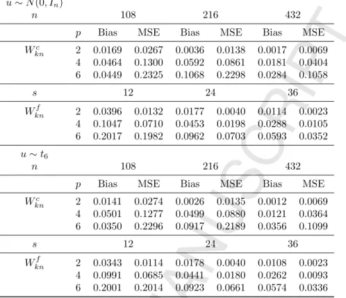
In this section we study the finite-sample properties of the estimates considered above in a Monte Carlo study, in two distinct settings considered earlier eg in Gupta and Robinson (2015). In the first setting, we consider Case (1991, 1992), where weight matrices take the ‘single nonzero diagonal block’ specification
Wknf =diag 0, . . . , Vm |{z} k−thdiagonal block , . . . ,0 , k= 1, . . . , p, (5.1)
withVm= (m−1)−1(lml0m−Im). In the second setting the weight matrices are
Wknc = (kWknk∗ )−
1
Wkn∗ , (5.2)
withW∗
kn the symmetric circulant matrix with first row elements given by
w∗1j,kn=
(
0 ifj= 1 orj=k+ 2, . . . , n−k;
1 ifj= 2, . . . , k+ 1 orj=n−k+ 1, . . . , n. (5.3)
ThusWc
kn is also a symmetric circulant matrix with first row elements given by w1∗j,kn/2k. In
both experiments we took p= 2,4,6. We first analyse the pure and intercept SAR cases. yn
was generated using (1.1) or (1.2) in each of the 1000 replications. We chose λ01 = 0.7, λ02 =
0.8, λ03= 0.5, λ04= 0.8, λ05= 0.4 andλ06= 0.3,when usingWknf while the values chosen when
using Wc
kn were λ01 = 0.1, λ02 = 0.2, λ03 = 0.2, λ04 = 0.1, λ05 = 0.1 and λ06 = 0.2 (because a
sufficient condition for S−1
n to exist in this case iskλk1 <1). One set ofui was generated as
u∼N(0, In)
n 108 216 432
p Bias MSE Bias MSE Bias MSE
Wc kn 2 0.0169 0.0267 0.0036 0.0138 0.0017 0.0069 4 0.0464 0.1300 0.0592 0.0861 0.0181 0.0404 6 0.0449 0.2325 0.1068 0.2298 0.0284 0.1058 s 12 24 36 Wknf 2 0.0396 0.0132 0.0177 0.0040 0.0114 0.0023 4 0.1047 0.0710 0.0453 0.0198 0.0288 0.0105 6 0.2017 0.1982 0.0962 0.0703 0.0593 0.0352 u∼t6 n 108 216 432
p Bias MSE Bias MSE Bias MSE
Wc kn 2 0.0141 0.0274 0.0026 0.0135 0.0012 0.0069 4 0.0501 0.1277 0.0499 0.0880 0.0121 0.0364 6 0.0350 0.2296 0.0917 0.2189 0.0356 0.1099 s 12 24 36 Wknf 2 0.0343 0.0114 0.0178 0.0040 0.0108 0.0023 4 0.0991 0.0685 0.0441 0.0180 0.0262 0.0093 6 0.2001 0.2014 0.0923 0.0661 0.0574 0.0336
Table 5.1: Monte Carlo (average) absolute bias and (average) MSE for PMLE, model (1.1)
fromt6(σ20= 3/2), having thicker tails.
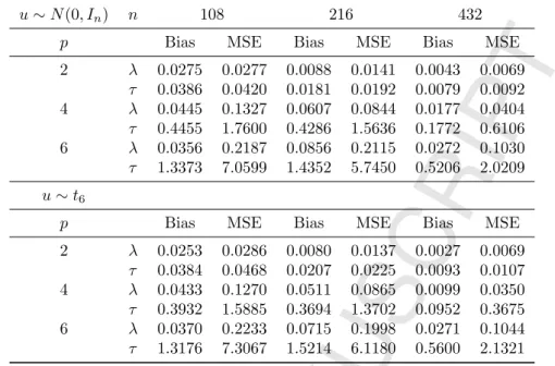
Tables 5.1 and 5.2 display Monte Carlo (absolute) bias and MSE for (1.1) and (1.2) respec-tively, withτ0= 1. Table 5.2 considers onlyWknc , the inclusion of an intercept not being possible
withWknf (cf Kelejian, Prucha, and Yuzefovich (2006)). Averages (averaging over bias and MSE for λ0i, i = 1, . . . , p) are reported for the spatial parameter estimates to conserve space. We
report results form= 16 (m= 8,24 were also simulated) only when usingWknf , and also take the number of districts s(implying n= 16s, and more generallyn =ms) to grow faster than
p. Indeed Theorems 2.3 and 2.4 indicate that whenmis either bounded or divergent the PMLE iss12/p12-consistent for the farmer-district setting, and in any case p2+
8 χm
4
χ/s+p4m/s→0 as
p, m, s → ∞ is necessary for (2.13) to hold asymptotically. We take s = 12,24,36, and this implies the need to combine spatial weight matrices by imposing the same spatial parameter for some blocks. Whenp= 2 we combine into two groups with six blocks, twelve blocks and eighteen blocks each whens= 12,24,36, respectively. Whenp= 4 (respectivelyp= 6) we combine into four groups (respectively six groups) with three, six and nine blocks each (respectively two, four and six blocks each). When usingWc
kn we taken= 108,216,432.
u∼N(0, In) n 108 216 432
p Bias MSE Bias MSE Bias MSE
2 λ 0.0275 0.0277 0.0088 0.0141 0.0043 0.0069 τ 0.0386 0.0420 0.0181 0.0192 0.0079 0.0092 4 λ 0.0445 0.1327 0.0607 0.0844 0.0177 0.0404 τ 0.4455 1.7600 0.4286 1.5636 0.1772 0.6106 6 λ 0.0356 0.2187 0.0856 0.2115 0.0272 0.1030 τ 1.3373 7.0599 1.4352 5.7450 0.5206 2.0209 u∼t6
p Bias MSE Bias MSE Bias MSE
2 λ 0.0253 0.0286 0.0080 0.0137 0.0027 0.0069 τ 0.0384 0.0468 0.0207 0.0225 0.0093 0.0107 4 λ 0.0433 0.1270 0.0511 0.0865 0.0099 0.0350 τ 0.3932 1.5885 0.3694 1.3702 0.0952 0.3675 6 λ 0.0370 0.2233 0.0715 0.1998 0.0271 0.1044 τ 1.3176 7.3067 1.5214 6.1180 0.5600 2.1321
Table 5.2: Monte Carlo absolute bias and MSE for PMLE, model (1.2), withWknc only.
either Wc kn or W
f
kn, although with the former the decline in bias is not necessarily monotonic.
Generally biases forWknf exceed those forWc
knbut MSEs and thus variances tend to be smaller.
Table 5.2 indicates a similar, non-monotonic, pattern of reduction for (1.2). However the bias and MSE for ˆτn can be very high for large p, eg for p = 6 they are unacceptable even when
n= 432.
Tables 5.3 and 5.4 similarly display Monte Carlo size and power for (1.1) and (1.2) respectively, with nominal size 5%. Power was computed using the false null hypothesis λi, τ = 0.5, for
each i. With Wc
kn in (1.1), size approaches the nominal value non-monotonically with n, but
with (1.2) the behaviour is rather more erratic. For p = 2 the oversizing is moderate, but dramatically worsens for p = 4,6. However in each case it gets closer to the nominal size as n increases, although not necessarily monotonically. On the contrary, with Wknf there is considerable undersizing. Larger values ofsgive little indication of an approach to the nominal 5%. The sizes are better for larger p, the best results arising when p= 6. The behaviour is similar across N(0,1) or t6 disturbances. On the other hand power increases monotonically in
each of the various settings, and would be much higher for thep= 4,6 cases if not forλ03= 0.5
(true under the false null), which effectively caps power at around 83%.
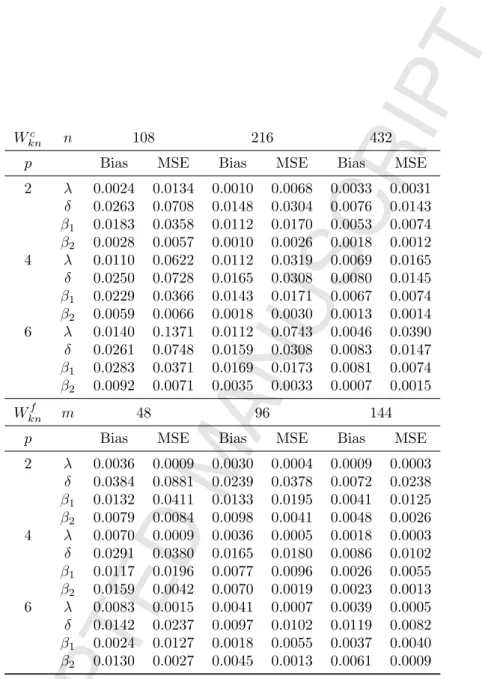
When generating yn using (1.3), we set kn = 2 and β01 = 1, β02 = 0.7. In Xn we took
xi1n(δ) = (ziδ1−1)/δ and xi2n(δ) = zi2, with (zi1, zi2)0 ∼U(0,5) (generated independently of
each other),i= 1, . . . , n, with 1000 replications, andδ0= 0.7. WithWknf equal blocks of sizem
were used, while three differentmwere chosen for each p: 48, 96 and 144. We also simulated a model withxi1n(δ) = eδzi1 andxi2n(δ) =zi2 and found similar results.
u∼N(0, In)
n 108 216 432
p Size Power Size Power Size Power
Wc kn 2 0.0475 0.5800 0.0460 0.7935 0.0400 0.9470 4 0.0660 0.2715 0.0998 0.4047 0.0760 0.5830 6 0.0335 0.1860 0.1197 0.3043 0.1027 0.4040 s 12 24 36 Wknf 2 0.0085 0.5835 0.0060 0.7805 0.0060 0.8855 4 0.0103 0.3520 0.0083 0.4925 0.0073 0.5867 6 0.0300 0.2035 0.0242 0.2807 0.0215 0.3422 u∼t6 n 108 216 432
p Size Power Size Power Size Power
Wc kn 2 0.0560 0.5695 0.0425 0.7970 0.0490 0.9480 4 0.0583 0.2745 0.0985 0.4233 0.0660 0.5775 6 0.0313 0.1818 0.1148 0.3062 0.1078 0.4085 s 12 24 36 Wknf 2 0.0090 0.5910 0.0060 0.7755 0.0070 0.8770 4 0.0123 0.3602 0.0067 0.4080 0.0070 0.5900 6 0.0303 0.2087 0.0230 0.2855 0.0237 0.3480
Table 5.3: Monte Carlo average size and average power for PMLE, model (1.1)
We now discuss the results for ˆθn in Tables 5.5 and 5.6, which report Monte Carlo bias and
MSE foru∼N(0, In) andu∼t6respectively. It is interesting to note that forWknf increasingm
mostly improves the estimates of the spatial parameters, for fixedp. However, Lee (2004) showed that the PMLE is inconsistent ifp= 1 whenmalone increases, while simulations conducted by Hillier and Martellosio (2013) also suggest convergence to a nondegenerate distribution. Similar results will undoubtedly apply if p >1, but fixed, andm alone increases. On the other hand, the block-diagonality of Wknf implies that the number of observations available to estimate the
λ0iincrease one-to-one withm. Generally bias and MSE improve with n, as expected. ForWknc
the results are as expected. Bias and MSE reduce with larger n and smallerp, and also with largernfor fixedp, and seem acceptable.
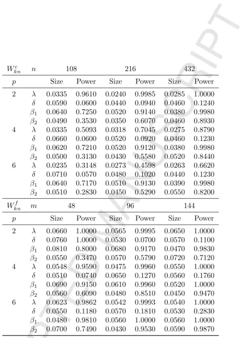
Tables 5.7 and 5.8 report Monte Carlo size and power foru∼N(0, In) andu∼t6respectively.
Now power is calculated using the incorrect null hypothesisθi= 0.6, for eachi. Under normality,
sizes when usingWknf are always between 4.3% and 8.2% but those forWc
knrange from 2.35% to
7.1%. When the disturbances are non-normal matters are similar, although there are instances (p= 2,6) of severe undersizing for λ0i withWknc that persists for all values of n. On the other
u∼N(0, In) n 108 216 432
p Size Power Size Power Size Power
2 λ 0.0275 0.5950 0.0088 0.8055 0.0043 0.9505 τ 0.0750 0.8460 0.0560 0.9920 0.0570 1.0000 4 λ 0.0445 0.2742 0.0607 0.4072 0.0177 0.5837 τ 0.2630 0.7070 0.2000 0.9320 0.1260 1.0000 6 λ 0.0356 0.1817 0.0856 0.2982 0.0272 0.4038 τ 0.4050 0.4960 0.5330 0.7830 0.2960 0.9110 u∼t6
p Size Power Size Power Size Power
2 λ 0.0253 0.5885 0.0080 0.8090 0.0027 0.9540 τ 0.0540 0.7950 0.0630 0.9720 0.0610 1.0000 4 λ 0.0433 0.2785 0.0511 0.4265 0.0099 0.5825 τ 0.2360 0.6210 0.1840 0.9100 0.0890 0.9920 6 λ 0.0370 0.1778 0.0715 0.2968 0.0271 0.4060 τ 0.4090 0.4820 0.5540 0.7680 0.2970 0.9920
Table 5.4: Monte Carlo size and power for PMLE, model (1.2), withWknc only.
Wc
kn but large m, p, for W f
kn, due to the increase in n afforded by increasingp. Power for δ0
tends to be low across the board, in part because its true value is 0.7 and the postulated value is 0.6. This factor doubtless also plays a role in the lower power for β02 generally as compared
to that forβ01.
Finally, Table 5.9 compares ˆθn with the IV estimate of Gupta and Robinson (2015) (denoted
ˇ
θn) whenWknc are employed,xi1n(δ) =zi1also (i.e. linear regressive SAR) and (zi1, zi2)∼U(0,1)
to match their design. We consider u generated from both N(0, In) and t6 distributions. We
report relative average MSE (RAMSE) separately for the autoregression and regression com-ponents, defining these as average MSE(ˆλn)/average MSE(ˇλn) and average MSE( ˆβn)/average
MSE( ˇβn), using the instruments {Wjnc zi1, Wjnc zi2}, j = 1, . . . , p. The PMLE does very well in
general. The IV estimates outperform the PMLE for the regression coefficientsβ01 and β02 in
4 out of 6 cases when p= 6, but fare much worse for the spatial parameters in all cases. Ex-periments in which the u were generated from a χ2
6−6 (this having σ02 = 12, and also being
non-symmetric) distribution followed the same pattern.
It is particularly interesting to note that the PMLE outperforms the IV estimate by such a large margin even when the disturbances are non-normal. A possible explanation for this is that the IV estimate relies on instruments derived from a power series expansion of S−1
n , and the
Wc
kn n 108 216 432
p Bias MSE Bias MSE Bias MSE
2 λ 0.0036 0.0110 0.0009 0.0053 0.0003 0.0028 δ 0.0184 0.0462 0.0212 0.0220 0.0016 0.0089 β1 0.0135 0.0238 0.0150 0.0116 0.0025 0.0049 β2 0.0018 0.0038 0.0002 0.0017 0.0002 0.0010 4 λ 0.0085 0.0546 0.0029 0.0268 0.0028 0.0132 δ 0.0176 0.0470 0.0215 0.0222 0.0018 0.0090 β1 0.0172 0.0242 0.0171 0.0116 0.0037 0.0049 β2 0.0048 0.0043 0.0010 0.0020 0.0006 0.0011 6 λ 0.0073 0.1186 0.0070 0.0648 0.0070 0.0312 δ 0.0194 0.0492 0.0221 0.0227 0.0023 0.0092 β1 0.0220 0.0251 0.0196 0.0118 0.0050 0.0050 β2 0.0068 0.0046 0.0024 0.0021 0.0010 0.0012 Wknf m 48 96 144
p Bias MSE Bias MSE Bias MSE
2 λ 0.0009 0.0002 0.0018 0.0003 0.0010 0.0002 δ 0.0038 0.0214 0.0090 0.0232 0.0090 0.0156 β1 0.0083 0.0264 0.0026 0.0129 0.0055 0.0078 β2 0.0042 0.0052 0.0066 0.0025 0.0032 0.0019 4 λ 0.0044 0.0006 0.0020 0.0003 0.0012 0.0002 δ 0.0129 0.0230 0.0070 0.0117 0.0023 0.0074 β1 0.0022 0.0129 0.0036 0.0061 0.0001 0.0040 β2 0.0109 0.0026 0.0059 0.0013 0.0022 0.0008 6 λ 0.0059 0.0010 0.0027 0.0005 0.0020 0.0003 δ 0.0142 0.0158 0.0037 0.0074 0.0046 0.0050 β1 0.0046 0.0079 0.0000 0.0040 0.0014 0.0028 β2 0.0087 0.0020 0.0039 0.0008 0.0028 0.0006
Table 5.5: Monte Carlo absolute bias and MSE for MLE (u ∼ N(0, In)), model (1.3) with
xi1n(δ) = (ziδ1−1)/δ.
Acknowledgements
We are grateful to an associate editor and three anonymous referees for constructive comments that led to an improved paper.
Wc
kn n 108 216 432
p Bias MSE Bias MSE Bias MSE
2 λ 0.0024 0.0134 0.0010 0.0068 0.0033 0.0031 δ 0.0263 0.0708 0.0148 0.0304 0.0076 0.0143 β1 0.0183 0.0358 0.0112 0.0170 0.0053 0.0074 β2 0.0028 0.0057 0.0010 0.0026 0.0018 0.0012 4 λ 0.0110 0.0622 0.0112 0.0319 0.0069 0.0165 δ 0.0250 0.0728 0.0165 0.0308 0.0080 0.0145 β1 0.0229 0.0366 0.0143 0.0171 0.0067 0.0074 β2 0.0059 0.0066 0.0018 0.0030 0.0013 0.0014 6 λ 0.0140 0.1371 0.0112 0.0743 0.0046 0.0390 δ 0.0261 0.0748 0.0159 0.0308 0.0083 0.0147 β1 0.0283 0.0371 0.0169 0.0173 0.0081 0.0074 β2 0.0092 0.0071 0.0035 0.0033 0.0007 0.0015 Wknf m 48 96 144
p Bias MSE Bias MSE Bias MSE
2 λ 0.0036 0.0009 0.0030 0.0004 0.0009 0.0003 δ 0.0384 0.0881 0.0239 0.0378 0.0072 0.0238 β1 0.0132 0.0411 0.0133 0.0195 0.0041 0.0125 β2 0.0079 0.0084 0.0098 0.0041 0.0048 0.0026 4 λ 0.0070 0.0009 0.0036 0.0005 0.0018 0.0003 δ 0.0291 0.0380 0.0165 0.0180 0.0086 0.0102 β1 0.0117 0.0196 0.0077 0.0096 0.0026 0.0055 β2 0.0159 0.0042 0.0070 0.0019 0.0023 0.0013 6 λ 0.0083 0.0015 0.0041 0.0007 0.0039 0.0005 δ 0.0142 0.0237 0.0097 0.0102 0.0119 0.0082 β1 0.0024 0.0127 0.0018 0.0055 0.0037 0.0040 β2 0.0130 0.0027 0.0045 0.0013 0.0061 0.0009
Table 5.6: Monte Carlo absolute bias and MSE for PMLE (u∼t6), model (1.3) withxi1n(δ) =
(zδ
Wc
kn n 108 216 432
p Size Power Size Power Size Power
2 λ 0.0335 0.9610 0.0240 0.9985 0.0285 1.0000 δ 0.0590 0.0600 0.0440 0.0940 0.0460 0.1240 β1 0.0640 0.7250 0.0520 0.9140 0.0380 0.9980 β2 0.0490 0.3530 0.0350 0.6070 0.0460 0.8930 4 λ 0.0335 0.5093 0.0318 0.7045 0.0275 0.8790 δ 0.0660 0.0600 0.0520 0.0920 0.0460 0.1230 β1 0.0620 0.7210 0.0520 0.9120 0.0380 0.9980 β2 0.0500 0.3130 0.0430 0.5580 0.0520 0.8440 6 λ 0.0235 0.3148 0.0273 0.4598 0.0263 0.6620 δ 0.0710 0.0570 0.0480 0.1020 0.0440 0.1230 β1 0.0640 0.7170 0.0510 0.9130 0.0390 0.9980 β2 0.0510 0.2830 0.0450 0.5290 0.0550 0.8200 Wknf m 48 96 144
p Size Power Size Power Size Power
2 λ 0.0660 1.0000 0.0565 0.9995 0.0650 1.0000 δ 0.0760 1.0000 0.0530 0.0700 0.0570 0.1100 β1 0.0810 0.8000 0.0680 0.9170 0.0470 0.9830 β2 0.0550 0.3470 0.0570 0.5790 0.0720 0.7120 4 λ 0.0548 0.9590 0.0475 0.9960 0.0550 1.0000 δ 0.0510 0.0740 0.0650 0.1270 0.0560 0.1760 β1 0.0690 0.9150 0.0610 0.9960 0.0520 1.0000 β2 0.0560 0.6090 0.0480 0.8510 0.0450 0.9470 6 λ 0.0623 0.9862 0.0542 0.9993 0.0540 1.0000 δ 0.0550 0.1180 0.0570 0.1810 0.0530 0.2830 β1 0.0480 0.9810 0.0560 1.0000 0.0560 1.0000 β2 0.0700 0.7490 0.0430 0.9530 0.0590 0.9870
Table 5.7: Monte Carlo size and power for MLE (u ∼ N(0, In)), model (1.3) with xi1n(δ) =
(zδ
Wknc n 108 216 432
p Size Power Size Power Size Power
2 λ 0.0265 0.9070 0.0260 0.9940 0.0185 1.0000 δ 0.0650 0.0660 0.0570 0.0550 0.0510 0.0950 β1 0.0650 0.5700 0.0600 0.8150 0.0400 0.9810 β2 0.0490 0.2540 0.0420 0.4620 0.0360 0.7820 4 λ 0.0238 0.4343 0.0240 0.6228 0.0245 0.8275 δ 0.0630 0.0670 0.0570 0.0550 0.0460 0.1030 β1 0.0640 0.5690 0.0530 0.8120 0.0390 0.9790 β2 0.0480 0.2360 0.0450 0.4260 0.0380 0.7330 6 λ 0.0135 0.2687 0.0215 0.3852 0.0227 0.5775 δ 0.0670 0.0680 0.0540 0.0600 0.0480 0.0970 β1 0.0620 0.5650 0.0560 0.8130 0.0400 0.9800 β2 0.0510 0.2220 0.0470 0.4010 0.0410 0.7130 Wknf m 48 96 144
p Size Power Size Power Size Power
2 λ 0.0735 0.9115 0.0770 0.9870 0.0620 0.9985 δ 0.0660 0.0650 0.0540 0.0710 0.0610 0.0750 β1 0.0630 0.5610 0.0500 0.7750 0.0620 0.9190 β2 0.0640 0.2580 0.0640 0.4300 0.0580 0.5610 4 λ 0.0665 0.9133 0.0643 0.9838 0.0560 0.9968 δ 0.0550 0.0700 0.0540 0.1020 0.0420 0.1230 β1 0.0590 0.7730 0.0540 0.9620 0.0390 0.9990 β2 0.0810 0.4700 0.0550 0.6900 0.0540 0.8090 6 λ 0.0602 0.9585 0.0555 0.9965 0.0513 0.9995 δ 0.0590 0.0780 0.0450 0.1220 0.0600 0.2270 β1 0.0620 0.9180 0.0380 0.9990 0.0530 1.0000 β2 0.0650 0.6240 0.0550 0.8270 0.0480 0.9550
Table 5.8: Monte Carlo size and power for PMLE (u∼t6), model (1.3) withxi1n(δ) = (zδi1−1)/δ.
n 108 216 432 108 216 432 p u∼N(0, In) u∼t6 2 λ 0.0472 0.0488 0.0507 0.0362 0.0287 0.0284 β 0.5212 0.5554 0.6202 0.4931 0.5028 0.5649 4 λ 0.0339 0.0413 0.0399 0.0239 0.0231 0.0233 β 0.4152 0.4706 0.5404 0.4630 0.4022 0.4357 6 λ 0.0353 0.0683 0.0601 0.0300 0.0536 0.0382 β 0.8069 3.5825 1.5249 0.9315 3.4552 1.3950
Table 5.9: Monte Carlo RAMSE between PMLE and IV withWc
Appendices
A
Proofs of theorems
Proof of Theorem 2.1. This is omitted as it can be deduced from the proof of Theorem 3.1 below, ignoring components of formulae and steps that are not relevant.
Proof of Theorem 2.2. In supplementary material.
We dropnsubscripts in the appendices. The following inequalities will be useful: kAk ≤ kAkF,
kAk2 ≤ kAkRkA0kR, kABkF ≤ kAkFkBk. In the sequel write ν = n1 2/a
1
2, where a is the
number of columns in Ψ. Thus in Section 2, a =porp+ 1, in Section 3, a= p+k+q and in Section 4, a =p+k. Further, for any matrix, vector E θ, σ2, ˜E denotes evaluation at a
generic estimateθ˜0,σ˜20 and ˜∆E = ˜E
−E. We can express (1.3) asy =Rλ0+Xβ0+uwith R= [W1y, . . . , Wpy]. Because Assumption 3 implies
y=S−1Xβ
0+S−1u, (A.1)
we have R =A+B, with B = [G1nu, . . . , Gpnnu], and for (1.1) the reduced form (A.1) holds with X = 0. The proofs of Theorems 3.3 and 3.4 should be read before the next two proofs, which are in any case in the supplementary appendix. We introduce them at this point to follow the order of the paper.
Proof of Theorem 2.3. In supplementary material.
Proof of Theorem 2.4. In supplementary material.
Proof of Theorem 2.5. This is omitted for the same reason as Theorem 2.1’s proof.
Proof of Theorem 2.6. This is similar to the proof of Theorem 2.3 and therefore omitted.
Proof of Theorem 3.1. The property βˆ−β0
→p 0 follows using arguments below, the closed form expression (see (3.2)) for ˆβ as a function of ˆγ,and the propertykˆγ−γ0k
p
→0,so we focus on proving the latter. From (3.4), (A.1)
Q(γ)− Q = logσ2(γ)/σ2−n−1log|T0(λ)T(λ)| = logσ2(γ)/σ2(λ) −logσ2/σ2 0+ logr(λ), (A.2) where σ2(λ) =n−1σ02kT(λ)k 2 F, σ 2=σ2(γ 0) =n−1u0M u,
using (3.3) and writingr(λ) =n−1 kT(λ)k2F/|T(λ)|2/n. From (A.1) σ2(γ) = n−1nS−10(Xβ0+u) o0 S0(λ)M(δ)S(λ)S−1(Xβ0+u) = c(γ) +d(γ) +e(γ), where c(γ) = n−1β00X0T0(λ)M(δ)T(λ)Xβ0, d(γ) = n−1σ02tr(T0(λ)M(δ)T(λ)), e(γ) = n−1tr T0(λ)M(δ)T(λ) uu0−σ20I + 2n−1β00X0T0(λ)M(δ)T(λ)u. Then logσ 2(γ) σ2(λ) = log σ2(γ) (c(γ) +d(γ))+ log c(γ) +d(γ) σ2(λ) = log 1 + e(γ) c(γ) +d(γ) + log 1 + c(γ)−f(γ) σ2(λ) , where f(γ) =n−1σ02tr(T0(λ) (I−M(δ))T(λ)).
Then from (A.2) and a standard kind of argument for proving consistency of implicitly defined extremum estimates Pkγˆ−γ0k ∈ N γ (η) = P inf γ∈ Nγ(η)Q (γ)− Q ≤0 ! ≤ P log 1 + sup γ∈ Nγ(η) c(γ) +e(γd)(γ) ! +log σ2/σ02 ≥ inf γ∈ Nγ(η) log 1 + c(γ)−f(γ) σ2(λ) + logr(λ) ! , where N γ(η) = Γ\Nγ(η), Nγ(η) =
{γ:kγ−γ0k< η;γ∈Γ}. From Assumptions 1 and 16
it follows that σ2/σ2 0
p
→1, so using log (1 +x) =x+o(x) asx→0 it suffices to show that as
n→ ∞ sup γ∈ Nnγ(η) c(γ) +e(γ)d(γ) p −→ 0, (A.3) sup γ∈ Nnγ(η) σf2((γλ)) −→ 0, (A.4) lim n→∞ inf γ∈ Nnγ(η) c(γ) σ2(λ)+ logr(λ) > 0. (A.5)
NowN γ(η)⊆nΛ× N δ(η/2)o∪nN λ(η/2)× Do, so inf γ∈ Nγ(η) c(γ) σ2(λ)+ logr(λ) ≥ min ( inf Λ×Nδ(η/2) c(γ) σ2(λ), inf Nλ(η/2) logr(λ) ) ≥ min ( inf Λ×Nδ(η/2) c(γ) C ,Nλinf (η/2) logr(λ) ) ,
from Assumption 6, whence Assumptions 7 and 16 imply (A.5). Again using Assumption 6, uniformly inγ,f(γ)/σ2(λ)
≤ |f(γ)|/cand
|f(γ)| ≤ CtrT0(λ)X(δ) (X0(δ)X(δ))−1X0(δ)T(λ)/n
= O tr(X0(δ)X(δ))/n2=O(k/n) uniformly, by Assumption 14, to check (A.4).
Finally consider (A.3). We first prove pointwise convergence. For any fixedγ∈ Nγ(η) and large enoughn,c(γ)≥ckβ0k2 from Assumption 16,d(γ)≥cbecause n−1σ02tr(T0(λ)T(λ))≥c
andtr(T0(λ) (I−M(δ))T(λ)) =O(k/n). Thuse(γ)/(c(γ) +d(γ)) =Op(|e(γ)|),wheree(γ) has mean 0 and variance
O kT0(λ)M(δ)T(λ)/nk2F + n X i=1 (t0i(λ)M(δ)ti(λ)/n)2+kβ00X0T0(λ)M(δ)T(λ)/nk 2 ! ,
whereti(λ) is theith column ofT(λ).SincekM(δ)k= 1 and Assumptions 4 and 12 imply (we
give a bound for the general case, that the same bound holds for the ‘single nonzero diagonal block’ case is simple to check)
kT(λ)k ≤CkS(λ)k ≤C max
i=1,...,pkWik kλk1=O(1), (A.6)
the first component is OkT(λ)/nk2F
=O n−1. The second one is O
n P i=1k ti(λ)k2/n2 =
OkT(λ)/nkF2=O n−1likewise. The final component isO
kXβ0/nk2
=Okβ0k2/n
=
O(k/n), from (3.6). Thus pointwise convergence is established.
To complete the proof of (A.3) we employ an equicontinuity argument. For arbitraryε >0 and finitely many γ∗ = (λ0
∗, δ0∗)0, the neighbourhoods kλ−λ∗k1 < ε× kδ−δ∗k < ε form a
sub-cover of the compact Γ = Λ× Din the product topology formed from the sum of k·k1 and
k·kdistances. It remains to prove that sup kλ−λ∗k1<ε×kδ−δ∗k<ε c(γ) +e(γd)(γ)− e(γ∗) c(γ∗) +d(γ∗) p −→0.
Write e(γ) c(γ) +d(γ)− e(γ∗) c(γ∗) +d(γ∗) = e(γ)−e(γ∗) c(γ) +d(γ) +e(γ∗) c(γ∗)−c(γ) +d(γ∗)−d(γ) (c(γ) +d(γ)) (c(γ∗) +d(γ∗))
whence, denoting the two components of e(γ) by e1(γ), e1(γ), the left side is bounded in
absolute value by |e1(γ)−e1(γ∗)| d(γ) + |e2(γ)−e2(γ∗)| c(γ) + |e(γ∗)| c(γ)c(γ∗)|c(γ∗)−c(γ)|+ |e(γ∗)| d(γ)d(γ∗)|d(γ∗)−d(γ)|. (A.7) We prove that sup kλ−λ∗k1<ε×kδ−δ∗k<ε |e2(γ)−e2(γ∗)| c(γ) p −→0. (A.8)
This part of the proof is relatively delicate due to both numerator and denominator increasing withk.The proof for the first term in (A.7) does not involve this feature and uses other arguments in the proof of (A.8). For the third term in (A.7),
|e(γ∗)| c(γ)c(γ∗)|c(γ∗)−c(γ)| ≤ |e(γ∗)| c(γ∗) 1 + c(γ∗) c(γ) p −→0
uniformly onkλ−λ∗k1< ε×kδ−δ∗k< ε,from the pointwise convergence ofe(γ)/(c(γ) +d(γ)) and the fact that numerator and denominator of c(γ∗)/c(γ) are uniformly of the same order
of magnitude, namely k, the result for the numerator being straightforward and that for the denominator a consequence of Assumption 16. The fourth term in (A.7) is uniformlyop(1) by similar arguments.
To prove (A.8), note that
e2(γ)−e2(γ∗) = 2n−1β00(X0(δ)T0(λ)M(δ)T(λ))−X0(δ∗)T0(λ∗)M(δ∗)T(λ∗))u, which can be written
2n−1β00
(X(δ)−X(δ∗))0T0(λ)M(δ)T(λ)
+X0(δ∗) (T0(λ)M(δ)T(λ)−T0(λ∗)M(δ∗)T(λ∗))}u. (A.9) The first of the two terms in braces has spectral norm bounded by kX(δ)−X(δ∗)k kT(λ)k2,
and by Assumption 15, kX(δ)−X(δ∗)k2≤ n X i=1 k X j=1 (xij(δ)−xij(δ∗))2=O knε2, (A.10)
for sufficiently smallkδ−δ∗k.
Thus due to kuk =Op n1/2, it follows that 2n−1β00(X(δ)−X(δ∗))
uniformlyOp kβ0kk1/2ε. Looking at the second term in braces in (A.9), writeT0(λ)M(δ)T(λ)− T0(λ
∗)M(δ∗)T(λ∗) as
(T(λ)−T(λ∗))0M(δ)T(λ) +T0(λ∗) (M(δ∗)−M(δ))T(λ) +T0(λ∗)M(δ∗) (T(λ)−T(λ∗)),
whose spectral norm is bounded by
kT(λ)−T(λ∗)k(kT(λ)k+kT(λ∗)k) +kT(λ∗)k kM(δ∗)−M(δ)k kT(λ)k = O(kT(λ)−T(λ∗)k+kM(δ∗)−M(δ)k). (A.11) Now kT(λ)−T(λ∗)k ≤ p X i=1 |λi−λ∗i| kWik S−1 ≤ C max i=1,...,pkWik kλ−λ∗k1≤Cε (A.12)
uniformly onkλ−λ∗k1 < ε× kδ−δ∗k < ε. RepresentingM(δ∗)−M(δ) as a sum of terms each with factorX(δ)−X(δ∗),or its transpose, with bounds for these typified by
n−1kX(δ)−X(δ∗)k(X0(δ)X(δ)/n)−1kX(δ)k,
wherekX(δ)k ≤Cn1/2,we deduce
kM(δ∗)−M(δ)k=O n−1/2
kX(δ)−X(δ∗)k=O k1/2ε,
from (A.10). Thus from (A.12), (A.11) has the same bound, so arguing much as before the contri-bution from the second term in braces in (A.9) isO kβ0kk1/2ε.Thus (A.9)=Op kβ0kk1/2ε,
and since Assumption 16 implies that as n → ∞, c(γ) ≥ ckβ0k2 uniformly and kβ0k−1 =
O k−1/2,the left side of (A.8) isO p
kβ0k−1k1/2ε
=Op(ε),whence (A.8) follows from arbi-trariness ofε,and the proof is completed.
Proof of Theorem 3.2. In supplementary material.
Proof of Theorem 3.3. Let ξ λ, σ2 denote the first derivative vector of (3.1), evaluated at λ, σ2. Defining Ry(θ) = Rλ+X(δ)β−y, the derivative of (3.1) at any admissible θ, σ2
is ξ θ, σ2= ϕ0(θ, σ2), 2σ−2n−1 Ry0(θ)X(δ), 2σ−2n−1 Ry0(θ) Π (θ)0, (A.13) where ϕ θ, σ2= 2σ−2n−1 σ2trG1(λ) +y0W10Ry(θ), . . . , σ2trGp(λ) +y0WpR0 y(θ)0. (A.14) Noting thatRy = −u, denotingCi=Gi+G0i and φ=σ0−2n−1 σ2 0trC1−u0C1u, . . . , σ20trCp−u0Cpu0, (A.15)