Practice of Epidemiology
Mediation Analysis With Intermediate Confounding: Structural Equation Modeling
Viewed Through the Causal Inference Lens
Bianca L. De Stavola*, Rhian M. Daniel, George B. Ploubidis, and Nadia Micali
*Correspondence to Dr. Bianca L. De Stavola, Department of Medical Statistics, London School of Hygiene and Tropical Medicine, Keppel Street, London WC1E 7HT, United Kingdom (e-mail: [email protected]).
Initially submitted January 2, 2014; accepted for publication August 11, 2014.
The study of mediation has a long tradition in the social sciences and a relatively more recent one in epidemiol-ogy. The first school is linked to path analysis and structural equation models (SEMs), while the second is related mostly to methods developed within the potential outcomes approach to causal inference. By giving model-free definitions of direct and indirect effects and clear assumptions for their identification, the latter school has formalized notions intuitively developed in the former and has greatly increased the flexibility of the models involved. However, through its predominant focus on nonparametric identification, the causal inference approach to effect decomposi-tion via natural effects is limited to settings that exclude intermediate confounders. Such confounders are naturally dealt with (albeit with the caveats of informality and modeling inflexibility) in the SEM framework. Therefore, it seems pertinent to revisit SEMs with intermediate confounders, armed with the formal definitions and ( parametric) iden-tification assumptions from causal inference. Here we investigate: 1) how ideniden-tification assumptions affect the specification of SEMs, 2) whether the more restrictive SEM assumptions can be relaxed, and 3) whether existing sensitivity analyses can be extended to this setting. Data from the Avon Longitudinal Study of Parents and Children (1990–2005) are used for illustration.
eating disorders; estimation by combination; G-computation; parametric identification; path analysis; sensitivity analysis
Abbreviations: ALSPAC, Avon Longitudinal Study of Parents and Children; BMI, body mass index; CDE, controlled direct effect; PNDE, pure natural direct effect; SEM, structural equation model; TNIE, total natural indirect effect.
The epidemiologic literature on causal inference is alight with contributions dedicated to the study of mediation. (A PubMed search for articles on mediation analysis in epidemi-ology produced 118“hits”for articles published in 2012 and 110“hits”for articles published in 2013.) The topic owes its origins, however, to an older body of literature that is well known in the social sciences. This school is often referred to as the“Baron and Kenny approach”(1,2) but is linked to Sewall Wright’s path analysis (3) and its extension, structural equation models (SEMs) (4). It includes several important publications that are less well known in the epidemiologic literature (5–10).
Contributions from the causal inference school have for-malized and generalized notions intuitively developed in the SEM school,first by defining (using potential outcomes)
precisely what is meant by direct and indirect effects, then by giving clear assumptions under which they can be identified, and lastly by generalizing the statistical methods available for carrying out such analyses to allow for nonlinearities, inter-actions, discrete outcomes, and semiparametric estimation (11–26).
With a few notable exceptions (11,27–29), the literature on natural direct and indirect effects focuses predominantly onnonparametric identification, which leads to the strong as-sumption of“no intermediate confounders”—that is, that no confounders (measured or unmeasured) of the mediator and outcome may be affected by the exposure. By relying on parametric models, however, such confounders are naturally dealt with in the SEM framework. Therefore, it is pertinent and timely to revisit SEMs with intermediate confounders,
– provided the original work is properly cited. December 11, 2014
armed with the formal definitions and ( parametric) identifi -cation assumptions from causal inference to reconcile the 2 approaches in this particular context.
In this article, we review how paths are traced in order to derive direct and indirect effects in simple linear SEMs which include intermediate confounders but exclude nonlinearities, and show their equivalence to the definitions based on poten-tial outcomes. We then investigate how different parametric assumptions for identification of the natural effects in the presence of intermediate confounders affect the specifi ca-tion of an extended SEM that includes nonlinearities. We further investigate whether the usual SEM assumption of
“no omitted influences”of any pair of variables in the sys-tem can be relaxed when estimation of the natural effects is the goal. Finally, we widen existing sensitivity analyses to the setting with intermediate confounding, exploiting the SEM framework.
THE 2 FRAMEWORKS Settings and aims
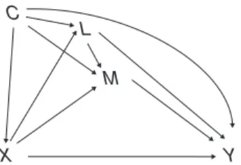
We will discuss settings involving an exposureX, an out-comeY, a mediatorM, background confounders Cof 1 or more of the relationshipsX-Y,M-Y, andX-M, and intermedi-ate confoundersLof theM-Yrelationship (Figure1). The aim is to separate the causal effect ofXacting along pathways that includeMfrom the causal effect ofXacting along other path-ways that do not involveM(theindirectanddirecteffects, respectively).
For simplicity, we letXbe a binary variable and assume that observations are not affected by missingness or measure-ment error.
The causal inference framework
The causal inference framework (11,12) invokespotential outcomes(30). For mediation analysis, these are:M(x), the potential value ofMifXhad been set, possibly counter to fact, to the valuex;Y(x,m), the potential value ofY ifX
had been set toxandMtom; andY(x,M(x′)), thecomposite
potential value ofYifXhad been set toxandMtoM(x′). Several definitions of direct and indirect effects have been proposed, with the choice depending on the causal question being addressed. We focus here on those most widely used and define them as linear contrasts, although definitions on other scales have been given (31–33).
Definitions
The controlled direct effect (CDE) ofXonYwhenMis controlled atm, CDE(m), and the pure natural direct effect (PNDE) ofXonY(11,12) are
CDEðmÞ ¼EfYð1;mÞg EfYð0;mÞg:
PNDE¼EfYð1;Mð0ÞÞg EfYð0;Mð0ÞÞg: CDE(m) is a comparison of 2 hypothetical worlds where, in thefirst,Xis set to 1 and, in the second,Xis set to 0, while in both worldsMis set tom. The PNDE is also a comparison of 2 hypothetical worlds whereXis set to 0 or 1 butMis set to take its naturalvalueM(0). Because in each of these com-parisonsMis set at the same value in both worlds (at least within the individual), they are measures of effects ofX un-mediated byM, that is,“direct.”
The complement of the PNDE is the total natural indirect effect (TNIE) ofXonY(11,34):
TNIE¼TCEPNDE
¼EfYð1;Mð1ÞÞg EfYð1;Mð0ÞÞg;
where TCE =E{Y(1)}−E{Y(0)} represents the total causal effect. The TNIE is a comparison of 2 hypothetical worlds in whichXis set to 1 in both, whileMchanges from its nat-uralvalue whenXis 1 to itsnaturalvalue whenXis 0. Intu-itively, this is an indirect effect, since it captures the part of the effect of XonY that is transmitted byM. There is no equivalent complement of CDE(m) (35).
Assumptions
In the absence of intermediate confounders. Identifi -cation of these estimands is possible if certain assumptions hold. Those most commonly invoked are specific versions of
no interference,consistency, andconditional exchangeability. Briefly, in the setting with no intermediate confounders and for CDE(m), the assumption of no interference states that an individual’s outcome is not influenced by the exposure sta-tus of another person (36–39) and also that the mediator value for one individual has no effect on the outcome in another. The assumption of consistency states that Y(x,m) equalsY
among subjects with observed exposure levelX=xand me-diator level M=m(40–43). The assumption of conditional exchangeability states that once individuals are stratified ac-cording to confoundersC, their allocation toXis essentially
“random”within these strata, and once they are stratified ac-cording toXandC, their allocation toMis essentially random within those strata. More formally, conditional exchange-ability states thatYðxÞ⊥⊥XjCandYðx;mÞ⊥⊥MjC;X, imply-ing no X-Y confounding conditionally on C and no M-Y
confounding conditionally onCandX(30,44). Under these extended assumptions, CDE(m) is nonparametrically identi-fied by regression standardization. For discreteC(45,46), CDEðmÞ ¼X c fEðYjX¼1;M¼m;C¼cÞ EðYjX¼0;M¼m;C¼cÞgPrðC¼cÞ: ð1Þ X Y M L C
Figure 1. Causal diagram for exposureX, mediatorM, outcomeY, background confounderC, and intermediate confounderL.
The sums here are replaced by integrals and Pr(C=c) by the corresponding density, ifCis continuous.
In order to identify the PNDE, the assumption of no inter-ference is expanded also to mean that the exposure of one individual has no effect on the mediator of another; the assump-tion of consistency is expanded also to mean thatM(x) =M
whenX=xand thatY(x,M(x)) =YwhenX=x(denoted gen-eralized consistencyorcomposition(46)); and the assump-tion of condiassump-tional exchangeability is expanded to mean that there is also noX-Mconfounding conditional onC (for-mally,MðxÞ⊥⊥XjC).
Under these extended assumptions, and whenMandCare discrete, the PNDE is nonparametrically identified (12,45, 46) by X c X m fEðYjX¼1;M ¼m;C¼cÞ EðYjX¼0;M¼m;C¼cÞg ×PrðM¼mjX¼0;C¼cÞPrðC¼cÞ: ð2Þ
The same assumptions are invoked to nonparametrically identify the TNIE, leading to (46)
TNIE¼X c X m EðYjX¼1;M¼m;C¼cÞ ×fPrðM ¼mjX¼1;C¼cÞ PrðM ¼mjX¼0;C¼cÞgPrðC¼cÞ: ð3Þ
For continuousC/M, summations are replaced by integrals and probabilities by density functions (see part A of the Web Appendix, available athttp://aje.oxfordjournals.org/). Equa-tions 2 and 3 are known as themediation formula(45).
In the presence of intermediate confounders. Identifying CDE(m) in the presence of intermediate confoundersLcan be achieved by adapting the assumption of no unaccounted
M-Yconfounding to include conditioning onLðYðx;mÞ⊥⊥ MjC;X;LÞand updating identification formula 1 (equation 1) to include the contribution viaL. This is commonly referred to as theG-computation formula(46,47) (Web Appendix, part B).
In contrast, identification of the natural effects, PNDE and TNIE, additionally involves some parametric restrictions on the relationships amongX,M,L, andY. Originally the restric-tion was stated by Robins and Greenland (11) as noX-M in-teraction at an individual level. Alternatively, Petersen et al. (27) suggested assuming that, conditional onC, the CDE does not vary withM(0). Under either of these additional parametric assumptions, PNDE and TNIE are identified by formulae that are extensions of equations 2 and 3. (Identifi ca-tion can also be obtained under certain“no-3-way-interaction” assumptions when the exposure is randomly assigned (48) or under no averageL-Minteraction in a nonparametric SEM with mutually independent errors (29).)
Estimation
Several approaches have been proposed for the estimation of these estimands, with standard errors typically obtained by
sandwich estimation or bootstrapping ( for a review, see Vansteelandt (46)). Among them, an extension of Robins’ (47) G-computation that incorporates the mediation formula posits regression models for each of the (conditional) expec-tations/probabilities/densities in the identifying equations, estimates their parameters (e.g., using maximum likelihood), and then plugs these estimates into the sums/integrals above (47,49). When the G-computation formula is too cumber-some to be evaluated analytically, the integration can be ap-proximated through Monte Carlo simulation (47,50) (see Appendix 2). The advantage of this approach is efficiency when all models are correctly specified, as well asflexibility. Essentially any combination of types (binary/categorical/ continuous) of outcomes, mediators, and intermediate con-founders can be modeled with little restriction on the as-sumed models, although the resulting complexities are a drawback (26).
To lessen the reliance on parametric modeling assumptions, many alternative semiparametric estimation approaches have been suggested, in particular G-estimation of structural nested models (21), inverse probability weighting of mar-ginal structural models (20), doubly and multiply robust methods that combine 1 or more of these approaches (24, 25), and multiply robust methods based on targeted maxi-mum likelihood (51).
The SEM framework
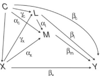
Unlike the above, the definitions of direct and indirect ef-fects given in the SEM literature depend on the specification of a particular statistical model (49). In the setting of Figure2 (with singleCandL), the following model for continuousY,
M, andLcould be specified:
L ¼γ0þγxXþγcCþϵl M¼α0þαxXþαlLþαcCþϵm Y ¼β0þβxXþβmMþβlLþβcCþϵy; 8 < : ð4Þ
whereXandC areexogenousvariables (no equations are specified for them),Y,M, andLareendogenous variables, andϵl,ϵm, andϵyare mean-zero error terms, uncorrelated with each other and with the exogenous variables. This is a linear path model for the joint distribution ofY,M, andL
(4,52). X Y M L C βx βm βc αx αc γx γc βl αl
Figure 2. Structural equation model for exposureX, mediatorM, out-comeY, background confounderC, and intermediate confounderL (error terms omitted for simplicity).
Sequentially replacing the expression forLinto the equation forMand that forMinto the equation forY, we obtain the reduced form of model 4 (equation 4):
Y ¼ ðβ0þα0βmþαlβmγ0þβlγ0Þ þ ðβxþαxβmþαlβmγxþβlγxÞX þ ðβcþαcβmþβlγcþαlβmγcÞCþ ðβmϵmþαlβmϵlþβlϵlþϵyÞ:
Here (βx+αxβm+αlβmγx+βlγx) is taken to represent thetotal causal effectofXonY. It can be partitioned into the direct (not mediated byM) and indirect (mediated) effects ofXbytracing the pathsin Figure2that make up the total effect (52). The indirect effect is found by multiplying the parameters along each of the (directed) paths fromXtoYthat includeMand summing them; here, this is (αxβm+γxαlβm). The direct effect is the sum of the remainder, (βx+γxβl). This is a more general version of theproduct of
coefficientsmethod (2,13,53).
Tracing the paths is possible only when the models for the endogenous variables are linear and do not include any interactions or other nonlinearities, although generalizations to settings with binary outcomes (via logit or probit regression) have been sug-gested, with standardization of the estimated parameters used to deal with their differences in scale across models (54). Other approaches within the SEM framework (i.e., without relying on counterfactuals) have also been proposed for general link func-tions and for models with interacfunc-tions and other nonlinearities (9,10,49,55), but these are only approximate and do not explicitly deal with settings with intermediate confounding.
Assumptions and estimation
Depending on the author, the identifying assumptions given in the SEM literature vary in detail, but essentially they are (5,7,8, 52,56):
1. Correct temporal order betweenX,L,M, andY.
2. “No omitted influences”(8), or“no lack of self-containment”(7), or“no other hidden relevant causes”(52). 3. Correct functional forms of each equation in the model.
4. Accurate measurements of all of the observed variables.
5. Error terms that are uncorrelated with each other and with the exogenous variables.
Thefirst 2 assumptions are structural, that is, causal, meaning that the regression equations fully reflect the underlying data-generating process and that they justify the apportioning of the mediation effects described above (7,8,52). For settings with intermediate confounders,“no omitted influences”is a stronger assumption than the conditional exchangeability assumption invoked in the causal inference literature, since it also involves noL-Yconfounding.
The last 3 assumptions are statistical. Thefirst refers to the linearity and additivity of the relationships among the variables, the second to the reliability of the available data, and the third to the behavior of the error terms. Requiring the error terms to be uncorrelated with each other and with the exogenous variables guarantees unbiased estimation of the model’s parameters via least squares. These estimated parameters can then be combined to obtain estimates of the direct and indirect effects, with measures of their precision obtained via the delta method (6) or bootstrapping (57). Importantly, departures from the statistical assumptions have repercussions for the structural ones. Correlated error terms—or correlated error terms and exogenous variables—would indicate departures from the structural assumption of no omitted relevant variables (52). Departures from the assumption of accurate measurements of the observed variables would lead to biased estimates of the model parameters and consequently of the medi-ation parameters (58).
Interestingly, the SEM literature does not mention the assumptions of no interference and consistency invoked by the causal inference literature, even though both are required for the estimated parameters to be interpreted as causal (59).
INSIGHTS
The causal inference estimands are defined in generality, although identification is achieved only parametrically when intermediate confounding is present. The SEM estimands are derived from specific parametric structural models that naturally include intermediate confounders. The 2 approaches are therefore very different, but they converge under certain scenarios. We believe that understanding their overlap when intermediate confounding is present can offer useful analytical insights.
Equivalence in estimands
The SEM approach to mediation applied to model 4 identifies the mediated effect ofXonYviaMas (αxβm+γxαlβm) and the nonmediated one as (βx+γxβl).
Under the same structural and parametric assumptions, the causal inference estimands can be written in closed form (see Web Appendix, part B):
PNDE¼ Z c Z l0 Z m Z l EðYjX¼1;M¼m;L¼l;C¼cÞfLðljX¼1;C¼cÞ EðYjX¼0;M¼m;L¼l;C¼cÞfLðljX¼0;C¼cÞ dl ×fMðmjL¼l0;X¼0;C¼cÞfLðl0jX¼0;C¼cÞdm dl0 fCðcÞdc ¼Z c Z l0 Z m ðβxþβlγxÞfMðmjL¼l0;X¼0;C¼cÞflðl0jX¼0;C¼cÞdm dl0 fCðcÞdc ¼βxþβlγx: CDEðmÞ ¼ Z c Z l EðYjX¼1;M¼m;C¼c;L¼lÞfLðljX¼1;C¼cÞdl Z l EðYjX¼0;M¼m;C¼c;L¼lÞfLðljX¼0;C¼cÞdl fCðcÞdc ¼ Z c ðβxþβlγxÞfCðcÞdc ¼βxþβlγx: TNIE¼ Z c Z l0 Z m Z l EðYjX¼1;M¼m;L¼l;C¼cÞfLðljX¼1;C¼cÞ ×ffMðmjX¼1;L¼l0;C¼cÞfLðl0jX¼1;C¼cÞ fMðmjX¼0;L¼l0;C¼cÞfLðl0jX¼0;C¼cÞ dl dm dl0 fCðcÞdc ¼Z c fβmðαxþαlγxÞ fCðcÞdc ¼βmðαxþαlγxÞ:
Hence the estimands from the 2 approaches coincide when the same parametric assumptions are made; likewise in the sim-ple setting without intermediate confounders (10,13,45,49). Although these equivalences apply only to linear SEMs that have no interactions or other nonlinear terms involvingX,
M, and L, closed-form solutions for the causal estimands above are not restricted to these simple models. Appendix 1 shows the closed-form solutions obtained for a more general linear SEM: L¼γ0þγxXþγcCþϵl M¼α0þαxXþαlLþαcCþαxlXLþϵm Y¼β0þβxXþβlLþβllL2þβmMþβmmM2 þβcCþβxlXLþβxmXMþϵy; 8 > > < > > : ð5Þ
where the residual terms are uncorrelated with each other and the explanatory variables in their equations and have constant variancesσ2 l,σ 2 m, andσ 2 y, respectively.
Parametric G-computation of the causal estimands above can then be achieved by combining the relevant estimated parameters of the assumed SEM, leading to what we refer to asestimation by combination(see Appendix 2 for its im-plementation in Mplus (Muthén and Muthén, Los Angeles, California); this implementation is more general than those in the papers by Valeri and VanderWeele (15) and
Emsley et al. (60), which deal only with settings without
L). Comparing the results obtained from analytical (i.e., by-combination) and Monte Carlo G-computation allows evalu-ation of the extent of the Monte Carlo error, as illustrated in the example.
Understanding the assumptions required for parametric identification
Identifiability of the natural direct and indirect effects in the presence of intermediate confounding involves some parametric restrictions on the relationships amongX,M,L, and Y. Specifically, Robins and Greenland (11) proposed the assumption of no individualX-Minteraction—formally, thatYð1;mÞ Yð0;mÞis the same for allm. For settings in which parametric models forY,M, andLare specified via lin-ear regression, this can be formally examined.
For example, consider model 5 (equation 5). Assuming it is correctly specified, we see that
Yð1;mÞYð0;mÞ ¼βxþβlðLð1ÞLð0ÞÞþβllðLð1Þ 2 Lð0Þ2Þ þβxlLð1Þþβxmm ¼βxþβlγxþβllfγ2xþ2γxðγ0þγcCþϵlÞg þβxlðγ0þγxþγcCþϵlÞþβxmm; –
and thus the Robins and Greenland assumption holds if and only ifβxm¼0:Note that, had our model forYincluded a term inLM, the Robins and Greenland assumption would also have constrained its coefficient (βlm) to be zero (in line with the constraint proposed by Tchetgen Tchetgen and VanderWeele (29)).
Petersen et al. (27) propose the alternative identifying as-sumption that, within levels ofC, the CDE does not vary with
M(0). Formally,
EfYð1;mÞ Yð0;mÞjMð0Þ ¼m;C¼cg
¼EfYð1;mÞ Yð0;mÞjC¼cg:
Again, assuming that model 5 is correct, we see that
Mð0Þ ¼αxþαlLð0Þ þαcCþϵm
¼αxþαlðγ0þγcCþϵlÞ þαcCþϵm: Conditional onC, therefore, we see that bothY(1,m)−Y(0,m) andM(0) are functions ofϵl, except whenβll¼βxl¼0:Note that, given our model, assuming thatγx= 0 (in place ofβll) or thatαl= 0 would be equivalent to assuming no intermediate confounding, which is why we do not consider them.
Thus, given this particular model, we have 2 options in the presence of intermediate confounders: Either we identify the PNDE and TNIE under the assumption thatβxm= 0 or we identify them under the assumption thatβll=βxl= 0. Hence, examining the significance of these parameters in an associ-ational model forYthat contains all of these terms should aid in the selection of identification assumptions.
Equivalence in assumptions
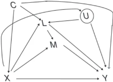
As we stated above, there is an interesting difference with regard to the identifying assumptions invoked by the 2 ap-proaches when the model involves intermediate confounders. Under the SEM, all of the error terms are assumed to be un-correlated with each other, a scenario which would not be sat-isfied were the L-Y relationship affected by unmeasured confounding, givenCandX(represented byUin Figure3). This is not a restriction invoked by the causal inference framework (as it concerns only confounding ofX-Y,X-M, andM-Y).
However, when the focus is identification of mediation effects within the SEM framework, the assumption of noL-Y
confounding is actually not required once the parametric as-sumptions discussed above are made (for a justification based on the theory described by Wermuth and Cox (61), see part C of the Web Appendix and—for a simpler setting—Moerkerke et al. (62); also see Pearl (63)). Thus, there is no contradiction in fitting a SEM without assuming noL-Yconfounding.
Sensitivity analyses
It is possible to perform simple sensitivity analyses of the assumption of no unmeasuredM-Yconfounding byfitting SEMs that allow for ϵy and ϵm to be correlated (10, 49, 64). We extend the sensitivity analysis of Imai et al. (49) to a setting with intermediate confounders—for example,
L¼γ0þγxXþϵl M¼α0þαxXþαlLþϵm Y¼β0þβxXþβmMþβlLþϵy; 8 < : ð6Þ
where, for simplicity, there are no confounders or interac-tion terms and the residuals are uncorrelated with the explan-atory variables in their equations and have constant variance (Var(ϵlÞ ¼VarðϵljXÞ ¼σ2l, VarðϵmÞ ¼VarðϵmjX;LÞ ¼
σ2
m, and VarðϵyÞ ¼VarðϵyjX;L;MÞ ¼σ2y)) but ϵm and ϵy are correlated with Corrðϵm;ϵyÞ ¼Corrðϵm;ϵyjX;L;MÞ ¼
ρ. This would occur in the presence of uncontrolled M-Y
confounding.
Now consider the alternative specification:
L¼γ0þγxXþϵl M¼α0þαxXþαlLþϵm Y¼β00þβ0xXþβ0lLþϵ0y; 8 < : ð7Þ
where the model for Y does not includeM and Varðϵ0yÞ ¼ Varðϵ0yjX;LÞ ¼σ0
2
y, and Corrðϵm;ϵ0yÞ¼Corrðϵm;ϵ0yjX;LÞ¼
ρ0. The parameters of model 6 (equation 6) are not identified
becauseβmandρare collinear, whereas the parameters of model 7 (equation 7) are.
Similarly to Imai et al. (49), we focus onρ′and interpret it as a measure of the strength of any unmeasuredM-Y con-founding that would imply an indirect effect of zero. Estimat-ingρ′is straightforward: Model 7 isfitted and the residuals are calculated, with their sample correlation being^ρ0. A confidence interval for^ρ0 is then obtained by bootstrapping (Stata code (StataCorp LP, College Station, Texas) given in Appendix 3).
RESULTS
To illustrate the advantages offitting SEMs when studying mediation, we analyze data on eating-disorder behaviors in adolescent girls. An adolescent eating-disorder study was carried out as part of the Avon Longitudinal Study of Parents and Children (ALSPAC), a birth cohort study of babies born between 1990 and 1992 in the South West of the United Kingdom (65). It involved data on eating-disorder behaviors collected by parental questionnaire on nearly 3,000 girls when they were around age 13.5 years. This information was used to identify 3 (standardized) latent scores for disordered eating patterns via factor analysis (66). For illustration, we
X Y
M
L U
C
Figure 3. Causal diagram for exposureX, mediatorM, outcomeY, intermediate confounderL, and unmeasured intermediateL-Y con-founderU. The circle aroundUindicates that it is unmeasured.
use one of these latent dimensions,“bingeing or overeating,” as the outcome of interest and study whether the influence of high maternal prepregnancy body mass index (BMI; weight (kg)/height (m)2; coded >25 for high and≤25 for low) is
mediated by the daughter’s BMI in childhood ( prospectively calculated from measurements taken at about age 7 years). It is of interest to separate the effects that maternal BMI may have through and not through potentially modifiable child-hood factors.
The assumed causal diagram is shown in Figure4, with maternal prepregnancy mental illness and education as back-ground confounders (C1andC2) and birth weight as an
inter-mediate confounder (L). The appropriate extension (i.e., incorporating the mediation formula) of the G-computation formula by Monte Carlo simulation was performed via the
gformulacommand in Stata 13 (50) (details given in Ap-pendix 2, part A); estimation by combination was performed afterfitting models by maximum likelihood in Mplus 7.11 (67) and combining the relevant estimated parameters as appropriate (details given in Appendix 2, part B). Standard errors were obtained via the bootstrap and delta methods, respectively.
Analyses are restricted to the 2,749 girls with complete data on all variables. Table1characterizes the data and shows marginal and partial correlations.“Bingeing or overeating”is both marginally and conditionally correlated with all other variables except maternal education, while maternal BMI (but not childhood BMI) is correlated with birth weight.
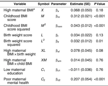
Table 2shows the estimated coefficients for the condi-tional expectation ofYexpressed without any of the paramet-ric constraints needed for identification in the presence of intermediate confounders. In particular, we allowed interac-tions betweenXandM,LandM, and nonlinearities inLand
Table 1. Mean Values/Percentages and Marginal (Above Main Diagonal) and Partial (Below Main Diagonal) Correlations for Variables Used in an Analysis of Eating-Disorder Behaviors Among Adolescent Girls (n= 2,749), Avon Longitudinal Study of Parents and Children, United Kingdom, 1990–2005a
Variable Symbol Mean (SD) %
Correlation Bingeing or
Overeating
Childhood
BMIb WeightBirth High MaternalBMI Low MaternalEducation Poor MaternalMental Health
Bingeing or overeating Y 0.00 (1.00) 1 0.33c 0.05c 0.06c −0.01 0.11c Childhood BMId M −0.02 (0.99) 0.34c 1 −0.02 0.26c 0.10c −0.02 Birth weighte L 0.10 (0.92) 0.05c 0.01 1 0.12c −0.04 −0.04
High maternal BMIf,g X 19 0.17c 0.31c 0.13c 1 0.17c −0.03
Low maternal educationg,h C1 55 0.04 0.13 c −0.03c 0.20c 1 0.04 Poor maternal mental healthg C2 13 0.11 c 0.01 −0.03 −0.01 0.04 1
Abbreviations: BMI, body mass index; SD, standard deviation.
aInformation on maternal education, prepregnancy BMI, and history of mental illness was obtained from postal questionnaires administered during pregnancy. Birth weight was measured at the time of birth. Childhood BMI was prospectively calculated from measurements taken at about age 7 years.
bWeight (kg)/height (m)2. c P< 0.05.
dChildhood BMI was age-standardized (leading to a standardized score). Because of missing values on other variables, its mean and SD were not exactly 0 and 1.
eBirth weight was internally standardized using the complete sample (leading to a standardized score). Because of missing values on other variables, its mean and SD were not exactly 0 and 1.
f Maternal prepregnancy BMI was dichotomized (<25, low;
≥25, high).
gPolychoric (or tetrachoric) correlations are reported when calculations involved this variable. hMaternal education was dichotomized:
“no high school”versus“at least high school.”
Maternal BMI Bingeing orOvereating
Childhood BMI Maternal Mental Illness,
Maternal Education
Birth Weight
Figure 4. Causal diagram for the relationships between high mater-nal prepregnancy body mass index (BMI; weight (kg)/height (m)2) (X), birth weight (L), offspring childhood BMI ( prospectively calculated from measurements taken at about age 7 years) (M), and off-spring“bingeing or overeating”score, measured at around age 13.5 years (Y), Avon Longitudinal Study of Parents and Children, United Kingdom, 1990–2005.
M. It appears that there is little evidence to rejectβxm= 0 (P= 0.76), while the evidence forβxlandβllbeing nonzero is greater (P= 0.08 andP= 0.01, respectively), suggesting that the Robins and Greenland assumption may be more plau-sible in this example. We nevertheless report the estimates of the mediation effects obtained under both assumptions in Table3(see also Web Table 1). The results suggest a strong mediated effect of high maternal BMI on“bingeing or over-eating”via childhood BMI, with a smaller direct effect captur-ing all other pathways. It appears therefore that more than 60% of the total effect of maternal overweight is transmitted via the daughter’s own size in childhood and not via other pathways, including birth weight, implicating a contribution of childhood environmental factors. Table3also highlights the closeness of the results obtained using Monte Carlo G-computation and G-G-computation via estimation by combi-nation; however, this required the size of the Monte Carlo sample to be increased to 100,000.
Sensitivity analyses show that a noncausal residual corre-lation between childhood BMI and“bingeing or overeating” would have to be very large, at least equal to 0.324 (95% con-fidence interval: 0.287, 0.361), to remove the path mediated by childhood BMI.
DISCUSSION
We have reviewed 2 alternative approaches to the study of mediation in settings with intermediate confounding. The one emerging from the SEM framework has a long tradition in the social sciences and uses definitions of direct and in-direct effects that are intuitive but are embedded within simple linear models. In contrast, the approach proposed within the causal inference literature is general, as it compares expected potential outcomes without reference to any particular model.
We have extended work done by others (10,13,45,49, 64) in deriving closed-form solutions to the identification equations for the causal inference estimands for general Table 3. Estimation of the Total Effect of High Maternal BMI on “Bingeing or Overeating”Among Adolescent Girls (n= 2,749) and of the Effects Mediated and Not Mediated by Childhood BMI (Estimation by Monte Carlo Simulation vs. Estimation by Combination), Avon Longitudinal Study of Parents and Children, United Kingdom, 1990–2005
Model and Estimand
Estimation Method and Estimate (SE) Monte Carlo G-Computationa Estimation by Combinationb Model 1c TCE 0.287 (0.052) 0.287 (0.049) PNDE 0.102 (0.050) 0.103 (0.047) TNIE 0.185 (0.021) 0.184 (0.019) CDE(0) 0.104 (0.050) 0.103 (0.047) Model 2d TCE 0.297 (0.052) 0.297 (0.049) PNDE 0.102 (0.051) 0.103 (0.051) TNIE 0.195 (0.031) 0.194 (0.028) CDE(0) 0.105 (0.049) 0.105 (0.049) Abbreviations: CDE, controlled direct effect; PNDE, pure natural direct effect; SE, standard error; TCE, total causal effect; TNIE, total natural indirect effect.
a Estimation by G-computation via Monte Carlo simulation was carried out using thegformulacommand (50) in Stata 13, with an enlarged Monte Carlo sample of 100,000 to increase agreement with closed-form results (see Appendix 2, part A); SEs were esti-mated via bootstrap.
b Estimation by combination was carried out by combining the maximum likelihood estimates of the relevant structural equation model parameters obtained in Mplus, version 7.11 (see Appendix 2, part B); SEs were estimated via the delta method.
c Model 1 follows the Robins and Greenland assumption (11) that there is no interaction betweenXandMat the individual level in their effects onY. The model was specified as follows. The equation for “bingeing or overeating”(Y) included childhood BMI (M; linear and quadratic terms), high maternal BMI (X; binary), birth weight (L; linear and quadratic terms), the interaction between high mater-nal BMI and birth weight, matermater-nal education (C1; binary), and pre-pregnancy mental health (C2; binary). The equation for childhood BMI included high maternal BMI (binary), birth weight (linear term), the interaction between high maternal BMI and birth weight, maternal education (binary), and prepregnancy mental health (binary). The equation for birth weight included high maternal BMI (binary), mater-nal education (binary), and prepregnancy mental health (binary).
d Model 2 follows the Petersen et al. assumption (27) that (con-ditional on C) the CDE does not vary with M(0). The model was specified as follows. The equation for“bingeing or overeating” in-cluded childhood BMI (linear and quadratic terms), high maternal BMI (binary), birth weight (linear term), the interaction between high maternal BMI and childhood BMI, maternal education (binary), and prepregnancy mental health (binary). The equation for childhood BMI included high maternal BMI (binary), birth weight (linear term), the interaction between high maternal BMI and birth weight, maternal education (binary), and prepregnancy mental health (binary). The equation for birth weight included high maternal BMI (binary), mater-nal education (binary), and prepregnancy mental health (binary). Table 2. Estimated Coefficients From a Regression Model for
“Bingeing or Overeating”Among Adolescent Girls (n= 2,749), Avon Longitudinal Study of Parents and Children, United Kingdom, 1990–2005
Variable Symbol Parameter Estimate (SE) PValue High maternal BMIa X βx 0.068 (0.050) 0.18 Childhood BMI score M βm 0.312 (0.021) <0.001 Childhood BMI score squared M2 βmm 0.043 (0.012) <0.001 Birth weight score L βl 0.034 (0.022) 0.13 Birth weight score
squared
L2 βll 0.032 (0.012) 0.01 High maternal
BMI × birth weight
XL βxl 0.078 (0.045) 0.08 High maternal
BMI × child BMI
XM βxm 0.014 (0.045) 0.76 Low maternal education C1 βc1 −0.011 (0.036) 0.76 Poor maternal mental health C2 βc2 0.207 (0.054) <0.001
Abbreviations: BMI, body mass index; SE, standard error. aWeight (kg)/height (m)2.
linear SEMs that include intermediate confounders. This has helped in clarifying the parametric assumptions needed for identification—and the consequent advantages of examining certain regression parameters, justifying the relaxation of the assumption of noL-Yunmeasured confounders made by the causal inference school and extending sensitivity analyses of unmeasuredM-Yconfounding. These results are novel and should help analysts investigating mediation in the presence of intermediate confounding. Although these results are re-stricted to settings that can be modeled with systems of linear equations, the insights gained here should also apply more generally, given the approximate closed-form expressions re-cently derived for binary outcomes and mediators (31,68) and the recent nonparametric identifying constraints involv-ingL-Minteractions (29,64).
ACKNOWLEDGMENTS
Author affiliations: Centre for Statistical Methodology, London School of Hygiene and Tropical Medicine, Univer-sity of London, London, United Kingdom (Bianca L. De Stavola, Rhian M. Daniel, George B. Ploubidis); and Institute of Child Health, Faculty of Population Health Sciences, Uni-versity College London, London, United Kingdom (Nadia Micali).
This work was partly funded by the Economic and Social Research Council (grants ES/I025561/1, ES/I025561/2, and ES/I025561/3), the Medical Research Council ( postdocto-ral fellowships G1002283 and 74882), the Wellcome Trust (grant 076467), and the University of Bristol (Bristol, United Kingdom), which provides core support for the Avon Longitudinal Study of Parents and Children (ALSPAC). N.M. was supported by a National Institute of Health Re-search clinician scientist award.
We are grateful to the midwives who helped to recruit the ALSPAC families and to the entire ALSPAC study team.
The views expressed in this publication are those of the authors and not necessarily those of the United Kingdom National Health Service, the National Institute for Health Research, or the United Kingdom Department of Health.
Conflict of interest: none declared.
REFERENCES
1. Judd CM, Kenny DA. Process analysis: estimating mediation in treatment evaluation.Eval Rev. 1981;5(5):602–619.
2. Baron RM, Kenny DA. The moderator–mediator variable distinction in social psychological research: conceptual, strategic, and statistical considerations.J Pers Soc Psychol. 1986;51(6):1173–1182.
3. Wright S. The method of path coefficients.Ann Math Stat. 1934;5(3):161–215.
4. Bollen KA. Causality and causal models. In:Structural Equations with Latent Variables. New York, NY: John Wiley & Sons, Inc.; 1989:40–79.
5. Duncan OD. Path analysis: sociological examples.AJS. 1966; 72(1):1–16.
6. Sobel ME. Asymptotic confidence intervals for indirect effects in structural equation models.Sociol Methodol. 1982;13:290–312.
7. James LR, Brett JM. Mediators, moderators, and tests for mediation.J Appl Psychol. 1984;69(2):307–321.
8. MacKinnon D. Single mediator model. In:Introduction to Statistical Mediation Analysis. New York, NY: Taylor & Francis; 2008:47–78.
9. Hayes AF, Preacher KJ. Quantifying and testing indirect effects in simple mediation models when the constituent paths are nonlinear.Multivariate Behav Res. 2010;45(4):627–660. 10. Muthén B.Applications of Causally Defined Direct and
Indirect Effects in Mediation Analysis Using SEM in Mplus. Los Angeles, CA: Muthén and Muthén; 2011.http://statmodel2.com/ download/causalmediation.pdf. Accessed August 8, 2014. 11. Robins JM, Greenland S. Identifiability and exchangeability for
direct and indirect effects.Epidemiology. 1992;3(2):143–155. 12. Pearl J. Direct and indirect effects. In:Proceedings of the
Seventeenth Conference on Uncertainty in Artificial Intelligence. San Francisco, CA: Morgan Kaufmann; 2001:411–420. 13. VanderWeele TJ, Vansteelandt S. Conceptual issues
concerning mediation, interventions and composition.Stat Interface. 2009;2(4):457–468.
14. VanderWeele TJ. Invited commentary: structural equation modeling and epidemiologic analysis.Am J Epidemiol. 2012; 176(7):608–612.
15. Valeri L, VanderWeele TJ. Mediation analysis allowing for exposure-mediator interactions and causal interpretation: theoretical assumptions and implementation with SAS and SPSS macros.Psychol Methods. 2013;18(2):137–150. 16. Emsley R, Dunn G, White IR. Mediation and moderation
of treatment effects in randomised controlled trials of complex interventions.Stat Methods Med Res. 2010;19(3):237–270. 17. Hafeman DM, VanderWeele TJ. Alternative assumptions for
the identification of direct and indirect effects.Epidemiology. 2011;22(6):753–764.
18. Ten Have TR, Joffe MM. A review of causal estimation of effects in mediation analyses.Stat Methods Med Res. 2012; 21(1):77–107.
19. Pearl J. Interpretable conditions for identifying direct and indirect effects. Los Angeles, CA: Department of Computer Science, University of California, Los Angeles; 2012. (Technical report R-389).
20. VanderWeele TJ. Marginal structural models for the estimation of direct and indirect effects.Epidemiology. 2009;20(1):18–26. 21. Robins JM. Testing and estimation of direct effects by
reparameterizing directed acyclic graphs with structural nested models. In: Glymour C, Cooper G, eds.Computation, Causation, and Discovery. Menlo Park, CA/Cambridge, MA: AAAI Press/The MIT Press; 1999:349–405. 22. Vansteelandt S. Estimating direct effects in cohort and
case-control studies.Epidemiology. 2009;20(6):851–860. 23. Joffe MM, Greene T. Related causal frameworks for surrogate
outcomes.Biometrics. 2009;65(2):530–538.
24. Goetgeluk S, Vansteelandt S, Goetghebeur E. Estimation of controlled direct effects.J R Stat Soc Series B Stat Methodol. 2008;70(5):1049–1066.
25. Tchetgen Tchetgen EJ, Shpitser I. Semiparametric theory for causal mediation analysis: efficiency bounds, multiple robustness and sensitivity analysis.Ann Stat. 2012;40(3):1816–1845. 26. Vansteelandt S, Bekaert M, Lange T. Imputation strategies for
the estimation of natural direct and indirect effects.Epidemiol Methods. 2012;1(1):131–158.
27. Petersen ML, Sinisi SE, van der Laan MJ. Estimation of direct causal effects.Epidemiology. 2006;17(3):276–284.
28. VanderWeele TJ, Vansteelandt S, Robins JM. Effect decomposition in the presence of an exposure-induced mediator-outcome confounder.Epidemiology. 2014;25(2): 300–306.
29. Tchetgen Tchetgen EJ, VanderWeele TJ. Identification of natural direct effects when a confounder of the mediator is directly affected by exposure.Epidemiology. 2014;25(2):282–291. 30. Rubin DB. Estimating causal effects of treatments in
randomized and nonrandomized studies.J Educ Psychol. 1974; 66(5):688–701.
31. VanderWeele TJ, Vansteelandt S. Odds ratios for mediation analysis for a dichotomous outcome.Am J Epidemiol. 2010; 172(12):1339–1348.
32. Vansteelandt S. Estimation of controlled direct effects on a dichotomous outcome using logistic structural direct effect models.Biometrika. 2010;97(4):921–934.
33. Martinussen T, Vansteelandt S, Gerster M, et al. Estimation of direct effects for survival data by using the Aalen additive hazards model.J R Stat Soc Series B Stat Methodol. 2011; 73(5):773–788.
34. Robins JM. Semantics of causal DAG models and the identification of direct and indirect effects. In: Green P, Hjort N, Richardson S, eds.Highly Structured Stochastic Systems. New York, NY: Oxford University Press; 2003:70–81. 35. VanderWeele TJ. Mediation and mechanism.Eur J Epidemiol.
2009;24(5):217–224.
36. Cox DR.Planning of Experiments. New York, NY: John Wiley & Sons, Inc.; 1958.
37. Rubin DB. Comment on:“Randomization analysis of experimental data in the Fisher randomization test”by D. Basu. J Am Stat Assoc. 1980;75(371):591–593.
38. Hudgens MG, Halloran ME. Toward causal inference with interference.J Am Stat Assoc. 2008;103(482):832–842. 39. Tchetgen Tchetgen EJ, VanderWeele TJ. On causal inference in
the presence of interference.Stat Methods Med Res. 2012; 21(1):55–75.
40. Hernán MA, Taubman SL. Does obesity shorten life? The importance of well-defined interventions to answer causal questions.Int J Obes (Lond). 2008;32(suppl 3): S8–S14.
41. Cole SR, Frangakis CE. The consistency statement in causal inference: a definition or an assumption?Epidemiology. 2009; 20(1):3–5.
42. VanderWeele TJ. Concerning the consistency assumption in causal inference.Epidemiology. 2009;20(6):880–883. 43. Pearl J. On the consistency rule in causal inference: axiom,
definition, assumption, or theorem?Epidemiology. 2010;21(6): 872–875.
44. Rubin DB. Bayesian inference for causal effects: the role of randomization.Ann Stat. 1978;6(1):34–58.
45. Pearl J. The mediation formula: a guide to the assessment of causal pathways in nonlinear models. In: Berzuini C, Dawid AP, Bernardinelli L, eds.Causality: Statistical Perspectives and Applications. Chichester, United Kingdom: John Wiley & Sons Ltd.; 2012:151–179.
46. Vansteelandt S. Estimation of direct and indirect effects. In: Berzuini C, Dawid AP, Bernardinelli L, eds.Causality: Statistical Perspectives and Applications. Chichester, United Kingdom: John Wiley & Sons Ltd.; 2012:126–150. 47. Robins J. A new approach to causal inference in mortality
studies with a sustained exposure period—application to control of the healthy worker survivor effect.Math Model. 1986;7(9-12):1393–1512.
48. Vansteelandt S, VanderWeele TJ. Natural direct and indirect effects on the exposed: effect decomposition under weaker assumptions.Biometrics. 2012;68(4):1019–1027.
49. Imai K, Keele L, Yamamoto T. Identification, inference and sensitivity analysis for causal mediation effects.Stat Sci. 2010; 25(1):51–71.
50. Daniel RM, De Stavola BL, Cousens SN. gformula: estimating causal effects in the presence of time-varying confounding or mediation using the g-computation formula.Stata J. 2011; 11(4):479–517.
51. Zheng W, van der Laan MJ. Targeted maximum likelihood estimation of natural direct effects.Int J Biostat. 2012;8(1). 52. Mulaik S. Structural equation models. In:Linear Causal
Modeling with Structural Equations. Boca Raton, FL: CRC Press; 2009:119–138.
53. MacKinnon DP, Warsi G, Dwyer JH. A simulation study of mediated effect measures.Multivariate Behav Res. 1995;30(1): 41–62.
54. MacKinnon DP, Dwyer JH. Estimating mediated effects in prevention studies.Eval Rev. 1993;17(2):144–158. 55. Muthén B, Asparouhov T. Causal effects in mediation
modeling: an introduction with applications to latent variables. Los Angeles, CA: Muthén and Muthén; 2014.http://www. statmodel.com/Mediation.shtml. Accessed November 19, 2014.
56. Bentler PM. Multivariate analysis with latent variables: causal modeling.Annu Rev Psychol. 1980;31:419–456.
57. MacKinnon D. Computer intensive methods for mediation models. In:Introduction to Statistical Mediation Analysis. New York, NY: Taylor & Francis; 2008:325–346. 58. Hoyle R, Kenny D.Sample Size, Reliability, and Tests of
Statistical Mediation. Thousand Oaks, CA: Sage Publications; 1999.
59. Hernán MA. Beyond exchangeability: the other conditions for causal inference in medical research.Stat Methods Med Res. 2012;21(1):3–5.
60. Emsley R, Liu H, et al. PARAMED: Stata module to perform causal mediation analysis using parametric models. St. Louis, MO: Federal Reserve Bank of St. Louis; 2013.
https://ideas.repec.org/c/boc/bocode/s457581.html. Accessed November 19, 2014.
61. Wermuth N, Cox DR. Distortion of effects caused by indirect confounding.Biometrika. 2008;95(1):17–33.
62. Moerkerke B, Loeys T, Vansteelandt S. Structural equation modeling versus marginal structural modeling for assessing mediation in the presence of post-treatment confounding. Psychol Methods. In press.
63. Pearl J.Interpretation and Identification of Causal Mediation. Los Angeles, CA: Department of Computer Science, University of California, Los Angeles; 2014.http://ftp.cs.ucla.edu/pub/ stat_ser/r389.pdf. Accessed August 8, 2014.
64. Imai K, Yamamoto T. Identification and sensitivity analysis for multiple causal mechanisms: revisiting evidence from framing experiments.Polit Anal. 2013;21(2):141–171.
65. Boyd A, Golding J, Macleod J, et al. Cohort profile: the ‘children of the 90s’—the index offspring of the Avon Longitudinal Study of Parents and Children.Int J Epidemiol. 2013;42(1):111–127.
66. Micali N, Ploubidis G, De Stavola B, et al. Frequency and patterns of eating disorder symptoms in early adolescence. J Adolesc Health. 2014;54(5):574–581.
67. Muthén LK, Muthén BO.Mplus User’s Guide. 7th ed. Los Angeles, CA: Muthén and Muthén; 1998.
68. Tchetgen Tchetgen EJ. Formulae for causal mediation analysis in an odds ratio context without a normality assumption for the continuous mediator. (Harvard University Biostatistics Working Paper no. 139). Berkeley, CA: Collection of Biostatistics Research Archive, Berkeley Electronic Press; 2012.http://biostats.bepress.com/cgi/viewcontent.cgi? article=1147&context=harvardbiostat. Accessed November 19, 2014.
APPENDIX 1
Estimation by Combination for a More General Linear SEM
Consider the following linear structural equation model (SEM):
L¼γ0þγxXþγcCþϵl M ¼α0þαxXþαlLþαcCþαxlXLþϵm Y ¼β0þβxXþβlLþβllL2þβmMþβmmM2þβcCþβxlXLþβxmXMþϵy; 8 < : ð8Þ
where the residual terms are uncorrelated with each other and the endogenous variables and have variancesσ2
l,σ
2
m, andσ
2
y, respectively. (Note that these variances are assumed to be constant, so that VarðϵljX;CÞ ¼σ2l, VarðϵmjX;L;CÞ ¼σ2m, and VarðϵyjX;L;M;CÞ ¼σ2y.)
For this model, the expression for the pure natural direct effect (PNDE) (see Web Appendix, part B), Z c Z l0 Z m Z l fEðYjX¼1;M ¼m;L¼l;C¼cÞfLðljX¼1;C¼cÞ EðYjX¼0;M¼m;L¼l;C¼cÞfLðljX¼0;C¼cÞgdl ×fMðmjL¼l0;X¼0;C¼cÞfLðl0jX¼0;C¼cÞdm dl0 fCðcÞdc; ð9Þ
can be written in closed form. Considerfirst its inner component: Z l fEðYjX¼1;M¼m;L¼l;C¼cÞfLðljX¼1;C¼cÞ EðYjX¼0;M¼m;L¼l;C¼cÞfLðljX¼0;C¼cÞgdl: This is equal to fβ0þβxþ ðβlþβxlÞL1ðcÞ þβllL21ðcÞ þβmmþβmmm 2þβ ccþβxmmg fβ0þβlL0ðcÞ þβllL20ðcÞ þβmmþβmmm 2þβ ccg ¼βxþβlðL1ðcÞ L0ðcÞÞ þβllðL21ðcÞ L20ðcÞÞ þβxlL1ðcÞ þβxmm; ð10Þ where LxðcÞ ¼EðLjX¼x;C¼cÞ ¼γ0þγxxþγcc L2 xðcÞ ¼EðL 2jX ¼x;C¼cÞ ¼ ðL xðcÞÞ2þσ2l L1ðcÞ L0ðcÞ ¼γx L2 1ðcÞ L20ðcÞ ¼ ðL1ðcÞÞ 2 ð L0ðcÞÞ 2¼ γ2 xþ2γxðγ0þγccÞ: Let AðcÞ ¼βxþβlγxþβllfγ2xþ2γxðγ0þγccÞg þβxlðγ0þγxþγccÞ: Writing equation 10 asA(c) +βxmm, we can rewrite equation 9 as
Z c Z l0 Z m ðAðcÞ þβxmmÞfMðmjL¼l0;X¼0;C¼cÞflðl0jX¼0;C¼cÞfCðcÞdm dl0dc ¼ Z c fAðcÞ þβxmM0ðcÞgfCðcÞdc ¼AþβxmM0; –
where MxðcÞ ¼EðMjX¼x;C¼cÞ ¼α0þαxxþ ðαlþαxlxÞLxðcÞ þαcc M0ðcÞ ¼α0þαlðγ0þγccÞ þαcc A¼ Z AðcÞfcðcÞdc ¼βxþβlγxþβllfγ2xþ2γxðγ0þγcμcÞg þβxlðγ0þγxþγcμcÞ M0¼ Z M0ðcÞfcðcÞdc ¼α0þαlðγ0þγcμcÞ þαcμc: Thus, equation 9 becomes
βxþβlγxþβllfγ2xþ2γxðγ0þγcμcÞg þβxlðγ0þγxþγcμcÞ þβxmfα0þαlðγ0þγcμcÞ þαcμcg:
If the model is correctly specified and if, additionally, the assumptions of no interference, strong consistency, and conditional exchangeability are met and one of the parametric assumptions described in the text is met, then this expression can be interpreted as the PNDE. However, note that the additional parametric assumptions constrain some of the parameters above to be zero, and thus the expression simplifies.
Similar calculations for CDE(m), the controlled direct effect (CDE) ofXonYwhenMis controlled atm(see Web Appendix, part B), lead to
CDEðmÞ ¼Aþβxmm
¼βxþβlγxþβllfγ2xþ2γxðγ0þγcμcÞg þβxlðγ0þγxþγcμcÞ þβxmm;
with the interpretation as CDE(m) being justified if the model is correctly specified and if the appropriate assumptions (no in-terference, consistency, conditional exchangeability) are met; note that the parametric restrictions described in the text are not required for this estimand.
Finally, for the total natural indirect effect (TNIE) (see Web Appendix, part B), we have the expression Z c Z l0 Z m Z l EðYjX¼1;M ¼m;L¼l;C¼cÞfLðljX¼1;C¼cÞ ×ffMðmjX¼1;L¼l0;C¼cÞfLðl0jX¼1;C¼cÞ fMðmjX¼0;L¼l0;C¼cÞfLðl0jX¼0;C¼cÞgfCðcÞdl dm dl0dc; which can be rewritten as
Z c fðβmþβxmÞðM1ðcÞ M0ðcÞÞ þβmmðM12ðcÞ M02ðcÞÞgfCðcÞdc; ð11Þ where M1ðcÞ M0ðcÞ ¼αxþαxlðγ0þγxþγccÞ þαlγx M2 1ðcÞ M 2 0ðcÞ ¼EðM 2jX¼ 1;C¼cÞ EðM2jX¼0;C¼cÞ ¼ fM1ðcÞg 2 f M0ðcÞg 2þ VarðMjX¼1;C¼cÞ VarðMjX¼0;C¼cÞ ¼ fα0þαxþ ðαlþαxlÞðγ0þγxþγccÞ þαccg 2 f α0þαlðγ0þγccÞ þαccg 2 þ ðαlþαxlÞ 2 σ2 l þσ 2 m ðα 2 lσ 2 l þσ 2 mÞ ¼ fα0þαlðγ0þγxþγccÞ þαccg2 þ2fα0þαlðγ0þγxþγccÞ þαccgfαxþαxlðγ0þγxþγccÞg þ ð2αlþαxlÞαxlσ2l: –
Thus, equation 11 can be rewritten as ðβmþβxmÞfαxþαxlðγ0þγxþγcμcÞ þαlγxg þβmmðfαxþαlγxþαxlðγ0þγxÞg 2 þ2ðα0þαlγ0Þfαxþαlγxþαxlðγ0þγxÞg þ2½ðα0þαlγ0Þαxlγcþ fαxþαlγxþαxlðγ0þγxÞgðαcþαlγcþαxlγcÞμc þ f2ðαcþαlγcÞ þαxlγcgαxlγcðμ 2 cþσ 2 cÞ þ ð2αlþαxlÞαxlσ2lÞ; whereσ2cis the variance ofC.
Again, this can be interpreted as the TNIE if the model is correctly specified and if, additionally, the assumptions of no in-terference, strong consistency, and conditional exchangeability are met and one of the parametric assumptions is met. Note again that the additional parametric assumptions constrain some of the parameters above to be zero, simplifying the expression.
APPENDIX 2
G-Computation in Stata and Mplus
y dependent variable
x exposure
m mediator
l intermediate confounder
c_1 first baseline confounder
c_2 second baseline confounder
m2 m2
l2 l2
xl x×l
xm x×m
A. G-computation by Monte Carlo simulations using Stata
To implement G-computation by Monte Carlo simulation, we have used the user-written commandgformula. The syntax used was as follows (for more details, refer to Daniel et al. (50)):
1. Model 1 (Robins and Greenland’s identifying assumptions (11)):
#delimit ;
gformula y x m m2 l l2 c1 c2 xl,
mediation outcome(y) exposure(x) mediator(m) post_confs(l) base_confs(c1 c2)
obe control( m:0)
commands(y:regress, m:regress, l:regress)
equations(y:x m m2 l l2 c1 c2 xl, m:x l c1 c2 xl, l:x c1 c2) derived(m2 l2 xl) derrules(m2:m*m,l2:l*l, xl:x*l)
minsim samples(1000) moreMC simulations(100000) replace seed(79); #delimit cr
2. Model 2 (Petersen et al.’s identifying assumptions (27)):
#delimit ;
gformula y x m m2 l l2 c1 c2 xl xm,
mediation outcome(y) exposure(x) mediator(m) post_confs(l) base_confs(c1 c2)
obe control( m:0)
commands(y:regress, m:regress, l:regress)
equations(y:x m m2 l c1 c2 xm, m:x l c1 c2 xl, l:x c1 c2)
derived(m2 l2 xl xm) derrules(m2:m*m,l2:l*l, xl:x*l, xm:x*m)
minsim samples(1000) moreMC simulations(100000) replace seed(79); #delimit cr
B. G-computation via estimation by combination using Mplus
The implementation with 2 confounders requires an extension of the expressions given in Appendix 1.
Letμc1andμc2be the mean values of the 2 confounders,σc21andσ2c1 their variances, andσ12their covariance. Also let L0¼γ0þ ðγc1μc1þγc2μc2Þ L1¼L0þγx P1¼α0þαlγ0 P2¼αxþαlγxþαxlðγ0þγxÞ A¼βxþβlγxþβllfγ2xþ2γxL0g þβxlL1 M0¼ fα0þαlL0þαc1μc1þαc2μc2g Pc1¼ ðαc1þαlγc1þαxlγc1Þμc1 Pc2¼ ðαc2þαlγc2þαxlγc2Þμc2: Then, CDEðmÞ ¼Aþβxmm PNDE¼AþβxmM0 TNIE¼ ðβmþβxmÞfαxþαxlL1þαlγxg þβmmðP 2 2þ2P1P2þ2½P1αxlγc1μc1þP2Pc1μc1þ2½P1αxlγc2μc2þP2Pc2μc2 þ ½2ðαc1þαlγc1Þ þαxlγc1αxlγc1ðμ 2 c1þσ 2 c1Þ þ ½2ðαc2þαlγc2Þ þαxlγc2αxlγc2ðμ 2 c2þσ 2 c2Þ þ ð½2ðαc1þαlγc1Þ þαxlγc2αxlγc1þ ½2ðαc2þαlγc2Þ þαxlγc1αxlγc2Þðμc1μc2þσ12Þ þ ð2αlþαxlÞαxlσ2lÞ:
The code below is for Mplus, version 7.11 (67), where we use the labeling options to identify the relevant parameters. 1. Model 1 (Robins and Greenland’s identifying assumptions (11)):
TITLE: Model 1
DATA: FILE IS“...”; Format is free; LISTWISE=ON;
VARIABLE: NAMES ARE id y x m m2 l l2 c_1 c_2 xl xm; USEV ARE y x m m2 l l2 c_1 c_2 xl; MISSING ARE .; IDVARIABLE= id; MODEL: [y] (beta0); y ON x (betax); y ON m (betam); y ON m2 (betamm); y ON l (betal); y ON l2 (betall); y ON c_1 (betac1); y ON c_2 (betac2); y ON xl (betaxl); [m] (alpha0); m ON x (alphax); m ON l (alphal); m ON c_1 (alphac1); m ON c_2 (alphac2); m ON xl (alphaxl); –
m (sigma2m); [l] (gamma0); l ON x (gammax); l ON c_1 (gammac1); l ON c_2 (gammac2); l (sigma2l); [c_1] (muc1); [c_2] (muc2); c_1 (sigma2c1); c_2 (sigma2c2); c_1 WITH c_2 (covc1c2); MODEL CONSTRAINT:
!this command lists all the terms used for the calculations !and gives them starting values:
NEW (betaxm*0 L0*.1 L1*.1 P1*.1 P2*.1 P_c1*.1 P_c2*.1
A_bar*.1 M_barbar_0*.1 cde0*.1 pnde*.1 tnie*.1 tce*0.1 ); !this is to remind ourselves of the Robins and Greenland assumption ! while using the general expressions
betaxm=0; !for CDE(0) L0 = gamma0+(gammac1*muc1+gammac2*muc2); L1 = gamma0+gammax+(gammac1*muc1+gammac2*muc2); A_bar=betax+betal*gammax+betall*(gammax*gammax+2*gammax*L0)+betaxl*L1; cde0=A_bar+betaxm*0; !for PNDE M_barbar_0=alpha0+alphal*L0+(alphac1*muc1+alphac2*muc2); pnde=A_bar+betaxm*M_barbar_0; !for TNIE P1=alpha0+alphal*gamma0; P2= (alphax +alphal*gammax+alphaxl*(gamma0+gammax)); P_c1=(alphac1+alphal*gammac1+alphaxl*gammac1)*muc1; P_c2=(alphac2+alphal*gammac2+alphaxl*gammac2)*muc2; tnie=(betam+betaxm)*(alphax+alphaxl*L1+gammax*alphal) + betamm*(P2*P2+2*P1*P2 +2*(P1*alphaxl*gammac1*muc1+P2*P_c1) +2*(P1*alphaxl*gammac2*muc2+P2*P_c2) +(2*(alphac1+alphal*gammac1)+alphaxl*gammac1)*alphaxl*gammac1* (muc1*muc1+sigma2c1) +(2*(alphac2+alphal*gammac2)+alphaxl*gammac2)*alphaxl*gammac2* (muc2*muc2+sigma2c2) +( (2*(alphac1+alphal*gammac1)+alphaxl*gammac1)*alphaxl*gammac2 +(2*(alphac2+alphal*gammac2)+alphaxl*gammac2)*alphaxl*gammac1 )*(muc1*muc2+covc1c2) +(2*alphal+alphaxl)*alphaxl*sigma2l ); tce=tnie+pnde; OUTPUT: SAMPSTAT ;
2. Model 2 (Petersen et al.’s identifying assumptions (27)):
TITLE: Model 2
DATA: FILE IS“...dat”; Format is free;
LISTWISE=ON;
VARIABLE: NAMES ARE id y x m m2 l l2 c_1 c_2 xl xm; USEV ARE y x m m2 l c_1 c_2 xm xl; MISSING ARE .; IDVARIABLE= id; MODEL: [y] (beta0); y ON x (betax); y ON m (betam); y ON m2 (betamm); y ON l (betal); y ON c_1 (betac1); y ON c_2 (betac2); y ON xm (betaxm); [m] (alpha0); m ON x (alphax); m ON l (alphal); m ON c_1 (alphac1); m ON c_2 (alphac2); m ON xl (alphaxl); m (sigma2m); [l] (gamma0); l ON x (gammax); l ON c_1 (gammac1); l ON c_2 (gammac2); l (sigma2l); [c_1] (muc1); [c_2] (muc2); c_1 (sigma2c1); c_2 (sigma2c2); c_1 WITH c_2 (covc1c2); MODEL CONSTRAINT:
NEW (betall*0 betaxl*0 L0*.1 L1*.1 P1*.1 P2*.1 P_c1*.1 P_c2*.1 A_bar*.1 M_barbar_0*.1
cde0*.1 pnde*.1 tnie*.1 tce*0.1 );
!this is to remind us of the Petersen et al assumptions ! while using the general expressions
betall=0; betaxl=0; !for CDE(0) L0 = gamma0+(gammac1*muc1+gammac2*muc2); L1 = gamma0+gammax+(gammac1*muc1+gammac2*muc2); A_bar=betax+betal*gammax+betall*(gammax*gammax+2*gammax*L0)+betaxl*L1; cde0=A_bar+betaxm*0; !for PNDE M_barbar_0=alpha0+alphal*L0+(alphac1*muc1+alphac2*muc2); pnde=A_bar+betaxm*M_barbar_0; !for TNIE P1=alpha0+alphal*gamma0; P2= (alphax +alphal*gammax+alphaxl*(gamma0+gammax)); P_c1=(alphac1+alphal*gammac1+alphaxl*gammac1)*muc1; P_c2=(alphac2+alphal*gammac2+alphaxl*gammac2)*muc2; tnie=(betam+betaxm)*(alphax+alphaxl*L1+gammax*alphal) + betamm*(P2*P2+2*P1*P2 +2*(P1*alphaxl*gammac1*muc1+P2*P_c1) –
+2*(P1*alphaxl*gammac2*muc2+P2*P_c2) +(2*(alphac1+alphal*gammac1)+alphaxl*gammac1)*alphaxl*gammac1* (muc1*muc1+sigma2c1) +(2*(alphac2+alphal*gammac2)+alphaxl*gammac2)*alphaxl*gammac2* (muc2*muc2+sigma2c2) +( (2*(alphac1+alphal*gammac1)+alphaxl*gammac1)*alphaxl*gammac2 +(2*(alphac2+alphal*gammac2)+alphaxl*gammac2)*alphaxl*gammac1 )*(muc1*muc2+covc1c2) +(2*alphal+alphaxl)*alphaxl*sigma2l ); tce=tnie+pnde; OUTPUT: SAMPSTAT ; APPENDIX 3 Stata—Sensitivity Analysis
Sensitivity analyses were carried out using theadofile calledsens_rho.ado, outlined below. Itfits a posited structural equation model (SEM), with an equation each forY,M, andL. In this example, itfits a model consonant with Robins and Greenland’s assumption (11). Note that the model forYdoes not includeMor any function ofMamong its explanatory variables, in order to allow for a correlation between the error terms of theYandMequations.
program define sens_rho, rclass version 13
preserve
cap matrix drop Psi
sem (y <- x l xl l2 c_1 c_2) (l<- x c_1 c_2) (m <- x l xl l2 c_1 c_2), \\\ nocapslatent cov(e.y*e.m)
qui estat framework, fitted matrix Psi=r(Psi)
matrix list Psi
scalar rho_dash=(Psi[3,1])/(sqrt(Psi[1,1]*Psi[3,3])) scalar list rho_dash
return scalar rho=rho_dash restore
end
It is best to check thatsens_rho.adopicks the right elements of the error term’s variance-covariance matrix by running the program once:
. sens_rho
Then, one needs to type
. bootstrap rho_dash=r(rho), reps(1000) saving(sens_rho,replace):sens_rho . estat bootstrap, all
to run the Statabootstrapcommand with 1,000 replications and see the results.