Statistics Publications
Statistics
7-8-2018
Integration of survey data and big observational
data for finite population inference using mass
imputation
Shu Yang
North Carolina State University
Jae Kwang Kim
Iowa State University, [email protected]
Follow this and additional works at:
https://lib.dr.iastate.edu/stat_las_pubs
Part of the
Statistical Methodology Commons, and the
Statistical Models Commons
The complete bibliographic information for this item can be found at
https://lib.dr.iastate.edu/
stat_las_pubs/258. For information on how to cite this item, please visit
http://lib.dr.iastate.edu/
howtocite.html.
This Article is brought to you for free and open access by the Statistics at Iowa State University Digital Repository. It has been accepted for inclusion in Statistics Publications by an authorized administrator of Iowa State University Digital Repository. For more information, please contact
Integration of survey data and big observational data for finite population
inference using mass imputation
Abstract
Multiple data sources are becoming increasingly available for statistical analyses in the era of big data. As an important example in finite-population inference, we consider an imputation approach to combining a probability sample with big observational data. Unlike the usual imputation for missing data analysis, we create imputed values for the whole elements in the probability sample. Such mass imputation is attractive in the context of survey data integration (Kim and Rao, 2012). We extend mass imputation as a tool for data integration of survey data and big non-survey data. The mass imputation methods and their statistical properties are presented. The matching estimator of Rivers (2007) is also covered as a special case. Variance estimation with mass-imputed data is discussed. The simulation results demonstrate the proposed estimators outperform existing competitors in terms of robustness and efficiency.
Keywords
Calibration weighting, Data fusion, Generalized additive model, Nearest neighbor imputation, Post stratification, Statistical matching
Disciplines
Statistical Methodology | Statistical Models
Comments
This pre-print is made available through arxiv:https://arxiv.org/abs/1807.02817.
arXiv:1807.02817v1 [stat.ME] 8 Jul 2018
Integration of survey data and big observational
data for finite population inference using mass
imputation
Shu Yang∗ and Jae Kwang Kim†
Abstract
Multiple data sources are becoming increasingly available for statistical analyses in the era of big data. As an important example in finite-population inference, we consider an imputa-tion approach to combining a probability sample with big observaimputa-tional data. Unlike the usual imputation for missing data analysis, we create imputed values for the whole elements in the probability sample. Such mass imputation is attractive in the context of survey data integration (Kim and Rao; 2012). We extend mass imputation as a tool for data integration of survey data and big non-survey data. The mass imputation methods and their statistical properties are presented. The matching estimator of Rivers (2007) is also covered as a special case. Vari-ance estimation with mass-imputed data is discussed. The simulation results demonstrate the proposed estimators outperform existing competitors in terms of robustness and efficiency.
Keywords: Calibration weighting; Data fusion; Generalized additive model; Nearest neighbor imputation; Post stratification; Statistical matching.
1
Introduction
In finite population inference, probability sampling is the gold standard for obtaining a representa-tive sample from the target population. Because the selection probability is known, the subsequent inference from a probability sample is often design-based and respect the way in which the data were collected. However, large-scale survey programs continually face heightened demands coupled with reduced resources. Demands include requests for estimates for domains with small sample sizes and desires for more timely estimates. Simultaneously, program budget cuts force reductions in sam-ple sizes, and decreasing response rates make nonresponse bias an important concern. Baker et al. (2013) and Keiding and Louis (2016) address the current challenges in using probability samples for finite population inferences.
∗Department of Statistics, North Carolina State University, North Carolina 27695, U.S.A. Email:
To meet the new challenges, statistical offices face the increasing pressure to utilize convenient but often uncontrolled big data sources, such as web survey panels and satellite information. While such data sources provide timely data for a large number of variables and population elements, they often fail to represent the target population of interest because of inherent selection biases.
To address new objectives and utilize modern data sources in statistically defensible ways, it is important to develop statistical tools for data integration for combining a probability sample with big observational data. To achieve this goal, one can apply mass imputation, where the imputed values are created for the whole elements in the probability sample. In the usual imputation for missing data analysis, the respondents in the sample provide a training dataset for developing an imputation model. In the proposed mass imputation, an independent big data sample is used as a training dataset, and mass imputation is applied to the probability sample. While the mass imputation idea for incorporating information from big data is very natural, the literature on mass imputation itself is very sparse. Breidt et al. (1996) discuss mass imputation for two-phase sampling. Kim and Rao (2012) develop a rigorous theory for mass imputation using two independent probability samples. Chipperfield et al. (2012) discuss composite estimation when one of the surveys is mass imputed. Rivers (2007) proposes a mass imputation approach using nearest neighbor imputation but the theory is not fully developed. Recently, Kim and Wang (2018), a technique report available by request from the authors, develop a theory for mass imputation for big data using a parametric model approach. However, the parametric model assumptions do not necessarily hold in practice. In order for mass imputation to be more useful and practical, the assumptions should be as weak as possible.
In this paper, we first develop a formal framework for mass imputation incorporating information from big data into a probability sample and present rigorous asymptotic results. Unlike Kim and Wang (2018), we do not make strong parametric model assumptions for mass imputation. Thus, the proposed method is appealing to survey practitioners. Our framework covers the nearest neighbor imputation estimator of Rivers (2007). In § 4, we investigate two strategies for improving the nearest neighbor imputation estimator, one using k nearest neighbor imputation and the other using generalized additive models. Secondly, using a novel calibration weighting idea, we propose an efficient mass imputation estimator and develop its asymptotic results. The efficiency gain is justified under a purely design-based framework and no model assumptions are used. The proposed methods are evaluated through extensive simulation studies based on artificial data and real-life data from U.S. Census Bureau’s Monthly Retail Trade Survey.
2
Basic Setup
2.1 Notation: two data sources
Let FN = {(Xi, Yi) : i ∈ U} with U = {1, . . . , N} denote a finite population, where Xi =
(X1
i, . . . , Xip) is a p-dimensional vector of covariates, and Yi is the study variable. We assume that FN is a random sample from a superpopulation model ζ, and N is known. Our objective is
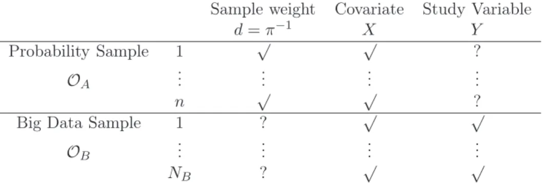
Table 1: Two data sources. “√” and “?” indicate observed and unobserved data, respectively. Sample weight Covariate Study Variable
d=π−1 X Y
Probability Sample 1 √ √ ?
OA ... ... ... ...
n √ √ ?
Big Data Sample 1 ? √ √
OB ... ... ... ...
NB ? √ √
Sample A is a probability sample, and Sample B is a big data but may have selection biases. to estimate the general finite population parameter µg=N−1PiN=1g(Yi) for some knowng(·). For example, if g(Y) = Y, µg = N−1PNi=1Yi is the population mean of Y. If g(Y) = I(Y < c) for some constantc,µg =N−1PiN=1I(Yi< c) is the population proportion of Y less than c.
Suppose that there are two data sources, one from a probability sample, referred to as Sample A, and the other from a big data source, referred to as Sample B. Table 1 illustrates the observed data structure. Sample A contains observations OA ={(di =πi−1, Xi) : i ∈ A} with sample size
n=|A|,where πi =P(i∈A) is known throughout Sample A, and Sample B contains observations OB = {(Xi, Yi) : i ∈ B} with sample size NB = |B|. Although the big data source has a large sample size, the sampling mechanism is often unknown, and we cannot compute the first-order inclusion probability for Horvitz-Thompson estimation. The naive estimators without adjusting for the sampling process are subject to selection biases. On the other hand, although the probability sample with sampling weights represents the finite population, it does not observe the study variable. 2.2 Assumptions
Let f(Y | X) be the conditional distribution of Y given X in the superpopulation model ζ. We define δB to be the indicator of selection to Sample B. We first make the following assumption. Assumption 1 (Ignorability) Conditional on X, the distribution of Y in Sample B follows the superpopulation model; i.e., f(Y |X;δB= 1) =f(Y |X).
Assumption 1 states the ignorability of the selection mechanism to Sample B conditional upon the covariates. This assumption is also a missingness at random assumption (Rubin; 1976).
Now, let f(X) and f(X | δB = 1) be the density function of X in the finite population and Sample B, respectively. We also require the following assumption.
Assumption 2 (Common support) The vector of covariates X has a compact and convex sup-port, with its density bounded and bounded away from zero. There exist constants Cl and Cu such
Assumption 2 implies that the support of X in Sample B is the same as that in the finite population. This assumption can also be formulated as a positivity assumption that P(δB = 1 |
X) > 0 for all X. This is necessary, because if the probability of selection into Sample B given some X is zero, then Sample B cannot provide adequate Y information for the units in this region without extrapolation.
3
Methodology
3.1 Nearest neighbor imputation
For estimation, ifYi were observed throughout Sample A, the Horvitz–Thompson estimatorµˆg,HT=
N−1Pi∈Aπi−1g(Yi)can be used. Our primary focus will be on the imputation estimator ofµg, given by µˆg,I =N−1Pi∈Aπi−1g(Yi∗),where Yi∗ is an imputed value forYi. Creating imputed values for the whole data is called mass imputation (Chipperfield et al.; 2012; Kim and Rao; 2012).
To find suitable imputed values, we consider nearest neighbor imputation; that is, find the closest matching unit from Sample B based on theX values and use the corresponding Y value from this unit as the imputed value. This approach has been called statistical matching by Rivers (2007). To investigate the theoretical properties, we first consider matching with replacement with single imputation; the discussion onk nearest neighbor imputation is presented in§ 4.
The nearest neighbor approach to mass imputation can be described in the following steps: Step 1. For each uniti∈A, find the nearest neighbor from Sample B with the minimum distance
betweenXj andXi. Leti(1)be the index of its nearest neighbor, which satisfiesd(Xi(1), Xi)≤
d(Xj, Xi), for j ∈ B, where d(Xi, Xj) is a distance function between Xi and Xj. Without loss of generality, we use the Euclidean distance, d(Xi, Xj) = ||Xi −Xj||, where ||X|| =
(XTX)1/2, to determine neighbors; our theoretical development applies to other distances (Abadie and Imbens; 2006).
Step 2. The nearest neighbor imputation estimator ofµg is
ˆ µg,nni= 1 N X i∈A π−i 1g(Yi(1)). (1)
The matching estimator is attractive in practice because it does not require parametric model assumptions. Secondly, it does not require Sample A and Sample B to have common units, but requires only Assumption 2. Assumption 2 ensures that for anyXi in Sample A, we can find a value
Xi(1) in Sample B that is arbitrarily close to Xi as NB → ∞. Then, by Assumption 1, g(Yi(1))
has the same distribution of g(Yi), given Xi. Moreover, for the same imputed dataset, one can estimate different parameters by choosing reasonable g(·). The main weakness of nearest neighbor imputation is that it is subject to the curse of dimensionality whenXis a vector, but such weakness is not applicable when the size of the matching donor pool is huge as in our big data setup.
3.2 Asymptotic results
To study the asymptotic properties of µˆg,nni, we impose the following regularity conditions on the
functional continuity and finite moments (e.g., Mack; 1981) and the sampling design for Sample A (Fuller; 2009, Ch. 1).
Assumption 3 (i) f(X) and µg(X) = E{g(Y) |X} are continuously differentiable for any
con-tinuous and bounded g(Y), and (ii) E{g(Y)β |X} is bounded for β = 0,1,2.
Assumption 4 (i) There exist positive constantsC1 andC2 such thatC1 ≤N n−1πi ≤C2,fori=
1, . . . , N; (ii) the sampling fraction for Sample A is negligible, nN−1 =o(1); and (iii) the sequence of
the Horvitz-Thompson estimatorsµˆg,HTsatisfiesvarp(ˆµg,HT) =O(n−1)and{varp(ˆµg,HT)}−1/2(ˆµg,HT−
µg) | FN → N(0,1) in distribution, as n→ ∞, where varp(·) is the variance under the sampling
design for Sample A.
We derive the asymptotic theory for µˆg,nni in the following theorem and defer its proof to the
Supplementary Material.
Theorem 1 Under Assumptions 1–3 andN NB−1=O(1), µˆg,nni has the same distribution asµˆg,HT
as NB→ ∞. Furthermore, under Assumption 4,µˆg,nni is consistent forµg, and
n1/2(ˆµg,nni−µg)→ N(0, Vnni), (2) where Vnni= lim n→∞ n N2E " varp ( X i∈A πi−1g(Yi) )# .
Theorem 1 implies that the standard point estimator can be applied to the imputed data{(Xi, Yi(1)) :
i ∈ A} as if the Yi(1)’s were observed values. Let πij be the joint inclusion probability for units
i and j. We show in the Supplementary Material that the direct variable estimator based on the imputed data ˆ Vnni= n N2 X i∈A X j∈A πij −πiπj πiπj g(Yi(1)) πi g(Yj(1)) πj .
is consistent for Vnni.
4
Other techniques for mass imputation
4.1 k-nearest neighbor imputation
Instead of using a single imputed value, we now consider fractional imputation with k imputed values for each missing outcome. Fractional imputation is designed to reduce the variance of the final estimator due to imputation (Kalton and Kish; 1984; Kim and Fuller; 2004).
Assume no matching ties, let Jk(i) be the set ofknearest neighbors for unit i Jk(i) = l∈B : X j∈B 1{d(Xj,Xi)≤d(Xl,Xi)} ≤k ={i(1), . . . , i(k)}.
The knearest neighbor approach to mass imputation can be described in the following steps: Step 1. For each unit i ∈ A, find the k nearest neighbors from Sample B, Jk(i). Impute the Y
value for unitiby µˆg(Xi) =k−1Pkj=1g(Yi(j)).
Step 2. Theknearest neighbor imputation estimator ofµg is
ˆ µg,knn= 1 N X i∈A πi−1µˆg(Xi).
In the nonparametric estimation literature, researchers have investigated the asymptotic properties of theknearest neighbor imputation estimators extensively. See, e.g., Mack and Rosenblatt (1979) and Mack (1981) for early references. Cheng (1994) established root-nconsistency of the knearest neighbor imputation estimator of the outcome mean when the outcome is subject to missingness. We derive the asymptotic theory for µˆg,knn in the context of mass imputation combining a probability
sample and a big data sample in the following theorem and defer its proof to the Supplementary Material.
Theorem 2 Under Assumptions 1–4, n(k/N)4/p→0, k/n→0, and k2/n→ ∞,
n1/2(ˆµg,knn−µg)→ N(0, Vknn), (3) where Vknn= lim n→∞ n N2 E " varp ( X i∈A π−i 1µg(Xi) )# +E 1−πB(X) πB(X) σg2(X) ! , andπB(X) =P(δB = 1|X).
If πB(X) goes to1,Vknn reduces to limn→∞ n/N2EvarpPi∈Aπ−i 1µg(Xi) . In this case,
Vknn is smaller than Vnni, suggesting that µˆg,knn gains efficiency over µˆg,nni. In finite samples,
Beretta and Santaniello (2016) conduct a simulation study to compare nearest neighbor imputation and k nearest neighbor imputation in the setting with independent and identically distributed data. They found that knearest neighbor imputation with a smallkoutperforms nearest neighbor imputation in terms of mean squared error.
4.2 Generalized additive models
Nearest neighbor imputation methods are nonparametric. On the other hand, parametric models especially linear models are sensitive to model misspecification. We now consider semiparamet-ric methods for mass imputation. Among semiparametsemiparamet-ric methods, generalized additive models
(Hastie and Tibshirani; 1990) are flexible regarding model specification of the dependence of Y on
X by specifying the model only through smooth functions rather than assuming a parametric re-lationship. We apply generalized additive models to leverage the predictive power of the big data sample to produce a predictive model for Y given X, so as to facilitate mass imputation for the probability sample.
We assume that g(Yi) givenXi follows some exponential family distribution, and
h−1{µg(Xi)}=f1(Xi1) +f2(Xi2) +· · ·fp(Xip), (4) where h(·) is an inverse link function, and each fk(·) is a smooth function ofXk, for k= 1, . . . , p. Model (4) allows for rather flexible specification of the dependence of Y on X. The estimated function fk(Xk) can reveal possible nonlinearities of the relationship ofY andXk.
There are several challenges in fitting model (4). First, fk(x) is an infinite-dimensional parame-ter, estimation of which often relies on some approximation. Second, we need to decide how smooth thefk(x) should be to balance the trade-off between model complexity and overfitting to the data at hand.
To solve the first issue, a common way to approximate fk(x) using splines. Let Bm(x) be the basis spline functions for m = 1, . . . , M (Ruppert et al.; 2009). We approximate fk(x) by
fk(x) =PMm=1γmkBm(x) with spline coefficients γmk. This leads to an approximation of model (4):
h−1[ ˆE{g(Yi)|Xi}] = p X k=1 M X m=1 γmkBm(Xik). (5)
In (5), a large M allows for increased model complexity and also an increased chance of overfit-ting; while a smallM may result in an inadequate model. This trade-off is balanced by choosing a relative largeMand then penalizing the model complexity in the estimation stage (Eilers and Marx; 1996). Let the vector of spline coefficients beγT
k = (γ1k, . . . , γmk)andγT= (γ1T, . . . , γpT). The estimate
ˆ
γ is obtained by maximizing the penalized likelihood: −2l(γ) +
p
X
k=1
λkγkTSkγk (6)
wherel(γ)is the log likelihood function ofγ,Skis a matrix with the(m, l)th componentR Bm′′(x)Bl′′(x)dx,
γT
kSkγk regularizes fk to be smooth for which the degree of smoothness is controlled by λk. Given the smoothing parameterλT= (λ
1, . . . , λp),the penalized likelihood function in (6) is optimized by a penalized version of the iteratively reweighted least squares algorithm (Nelder and Baker; 1972; McCullagh; 1984) to obtain γˆ. Regarding the choice of λ, we note that λ controls the trade-off between model complexity and overfitting, which can be estimated separately from other model co-efficients using generalized cross-validation or estimated simultaneously using restricted maximum likelihood estimation (Wood; 2006). In practice, the model performance is not sensitive to the choice of the number of basis functions, but rather estimation of the smoothing parameter is critical to
control the model complexity.
Once fitting the model, we can create an imputed value for each element iin Sample A as
ˆ
µg,GAM(Xi) =h{fˆ1(Xi1) + ˆf2(Xi2) +· · ·fˆp(Xip)},
where fˆk(x) = PMm=1γˆmkBm(x) for k = 1, . . . , p. The mass imputation estimator based on the generalized additive model is
ˆ µg,GAM= 1 N X i∈A π−i 1µˆg,GAM(Xi).
Because in our context, the sample size of Sample B is much larger than that of Sample A, the estimation error in the imputation model can be negligible compared to the sampling variability of
ˆ µg,GAM.
To close this subsection, it is worth commenting on the assumption of additive effects of X in model (4). This assumption may be fairly strong one. To relax the additivity assumption, we can extend model (4) to include interactions through using the tensor product basis. For example, we can include a bivariate interaction surfacef12(X1, X2) =PMm=1
PL
l=1γmlBm(X1)Bl(X2).
5
Regression calibration
In practice, especially for government agencies, one nearest neighbor may be preferred because of its simplicity in implementation and data storage. We now consider another strategy to improve the efficiency forµˆg,nni when additionally the membership to Sample B can be determined throughout
Sample A with the indicator δB. We can obtain δB by matching or directly asking about the membership to Sample B. The key insight is that the subsample of units in Sample A with δB = 1 constitutes a second-phase sample from Sample B, where Sample B acts as a new population.
Let h(δB, X, Y) be a multi-dimensional function of δB, δBX and δBY, e.g., h(δB, X, Y) =
(δB,1−δB, δBX, δBY)T. For simplicity of notation, we usehi to denoteh(δBi, Xi, Yi). We can cal-culate the population quantity H =N−1PN
i=1hi from Sample B. This insight enables the typical calibration weighting in survey sampling with known marginal totals. In Sample A, we treat the im-puted values as observed values, and the design weighted estimator ofH isHˆA=N−1Pi∈Aπi−1hi. In general, HˆA is not equal toH. We can use the known information H to improve the efficiency of µˆg,nni.
This suggests the following calibration strategy. We modify the original design weights{di :i∈
A} inµˆg,nni to a new set of weights{ωi:i∈A} by minimizing a distance function
X i∈A G(ωi, di) = X i∈A di ωi di − 1 2 , (7)
subject to the calibration constraints N−1P
be called generalized regression weights.
The proposed estimator utilizing the new set of weights is
ˆ µg,RC= 1 N X i∈A ωig(Yi(1)), (8)
which is asymptotically equivalent to a generalized regression estimator (Park and Fuller; 2012). We derive the asymptotic theory for µˆg,RC in the following theorem and defer its proof to the
Supplementary Material.
Theorem 3 Under Assumptions 1–4,
n1/2(ˆµg,RC−µg)→ N(0, VRC), (9) in distribution, as n→ ∞, where VRC= lim n→∞ n N2E varp " X i∈A πi−1{g(Yi)−hTiβN} #! , and βN =PNi=1hihTi −1PN i=1hig(Yi).
The calibrated estimator µˆg,RC improves the efficiency ofµˆg,nniin the sense that VRC is at most
as large as Vnni given in Theorem 1. Moreover, µˆg,RC is robust in the sense that we do not require
any modeling assumption.
Remark 1 (Choice of distance functions) Different distance functions in (7) can be consid-ered. If we chooseG(ωi, di) =−dilog(ωi/di), it leads to empirical likelihood estimation (Newey and Smith;
2004). If we choose the Kullback–Leibler distance function G(ωi, di) =ωilog(di/ωi), it leads to
ex-ponential tilting estimation (Kitamura and Stutzer; 1997; Imbens et al.; 1998; Schennach; 2007). Under mild conditions, these procedures provide a set of weights that is asymptotically equivalent to the set of regression weights (Deville and Särndal; 1992; Breidt and Opsomer; 2017).
For variance estimation, by Theorem (3), we construct a consistent variance estimator forµˆg,RC
asVbRC/n, where b VRC= n N2 X i∈A X j∈A πij−πiπj πij ˆ ei πi ˆ ej πj ,
witheˆi=g(Yi(1))−hTiβˆ, and
ˆ β= N X i=1 hihTi !−1 PN i=1δBig(Yi) P i∈Aπi−1(1−δBi)g(Yi(1)) PN i=1δBiXig(Yi) PN i=1δBiYig(Yi) .
6
Empirical experiments
In this section, we evaluate the finite sample performance of the proposed estimator using simulation studies, one based on artificial data and the other based on a synthetic population file from a single month sample of the U.S. Census Bureau’s Monthly Retail Trade Survey.
6.1 A simulation study
We generate the data according to the following mechanism. We first generate a finite population FN = {Xi = (X1i, X2i), Yi = (Y1i, Y2i) : i = 1, . . . N} with size N = 1,000,000, where Y1i is a continuous outcome and Y2i is a binary outcome. From the finite population, we select a big data sample B where the inclusion indicator δBi ∼Ber(pi) with pi the inclusion probability for unit i, and we obtain a representative sample A of size n = 1,000 using simple random sampling. The parameters of interest are the population mean N−1PNi=1Yi and the conditional population mean of Y1 givenY2= 1.
For generating the finite population, we consider linear models
Y1i = 1 +X1i+X2i+αi+ǫi, (10)
P(Y2i = 1|X1i, X2i;αi) = logit(1 +X1i+X2i+αi), and nonlinear models
Yi = 0.5(X1i−1.5)2+X22i+αi+ǫi, (11)
P(Y2i= 1|X1i, X2i;αi) = logit0.5(X1i−1.5)2+X22i+αi ,
whereX1i∼ N(1,1),X2i∼Exp(1),αi ∼ N(0,1),ǫi ∼ N(0,1), andX1i,X2i,αiandǫiare mutually independent. The variablesαi induce the dependence ofY1iandY2i even adjusting forX1i andX2i. For the big-data inclusion probability, we also consider a logistic linear model
logit(pi) =X2i, (12)
and a nonlinear logistic model
logit(pi) =−3 + (X1i−1.5)2+ (X2i−2)2. (13)
We consider the following combinations: I. (10) and (12); II. (10) and (13); II. (11) and (12); and IV. (11) and (13) for data generating mechanisms. Therefore, the simulation setup is a 2×2 factorial design with two levels in each factor.
Kim and Wang (2018) proposed the inverse propensity score weighting estimator using the estimated probability of selection into Sample B and the double robust estimator which further incorporates an outcome regression model. To evaluate the robustness and efficiency, we compare
the following estimators:
1. µˆHT, the Horvitz–Thompson estimator assuming the Yi’s were observed in Sample A for the purpose of benchmark comparison;
2. µˆipw, the inverse propensity score weighting estimator,
ˆ µipw = 1 N X i∈B 1 pi(ˆη) Yi(1),
where pi(η) = P(δBi = 1 |Xi;η) is a logistic regression model with a linear predictor X2i as a working model, and ηˆis an estimator of η based on Sample A;
3. µˆdr, the double robust estimator,
ˆ µdr= 1 N X i∈B 1 pi(ˆη) Yi(1)−XiTβˆ + 1 n X i∈A XT i β,ˆ
where βˆ is the estimated regression coefficients using (10) as the working outcome regression model based on Sample B;
4. µˆnni, the nearest neighbor imputation estimator;
5. µˆknn, the k nearest neighbor imputation estimator withk= 5;
6. µˆGAM, the generalized additive model imputation estimator;
7. µˆRC, the regression calibration estimator based onµˆnniwith calibration variablesH(δB, X, Y) =
(δB,1−δB, δBX, δBY)T.
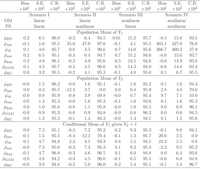
All simulation results are based on 1,000 Monte Carlo runs. Table 2 summarizes the simulation results with biases, standard errors, and coverage rates of95%confidence intervals using asymptotic normality of the point estiamtors. The following observations can be made from Table 2. µˆipw has
large biases when the propensity score is misspecified. µˆdr gains robustness over µˆipw if one of the
outcome regression model or the propensity score is correctly specified. However, if both models are misspecified, µˆdr has a larger bias. µˆnni has small biases across four scenarios, which shows its
robustness. Importantly, the performance ofµˆnni is close to that ofµˆHTin terms of standard errors
and coverage rates, which is consistent with our theory in Theorem 1. Moreover, as predicted by our theoretical results,µˆknn improves µˆnni in terms of efficiency. Also, µˆGAM shows robustness because
of the flexibility of the model specification. The regression calibration estimator µˆRC has small
biases across all scenarios and therefore shows robustness against model specifications for sampling score and outcome. Moreover, it has smaller standard errors than bothµˆnniandµˆknn. The coverage
Table 2: Simulation results: bias, standard error, and coverage rate of 95% confidence intervals under four scenarios based on 1,000 Monte Carlo samples. OM: outcome model; PS: propensity score model
Bias S.E. C.R. Bias S.E. C.R. Bias S.E. C.R. Bias S.E. C.R.
×102 ×102 ×102 ×102 ×102 ×102 ×102 ×102 ×102 ×102 ×102 ×102
Scenario I Scenario II Scenario III Scenario IV
OM linear linear nonlinear nonlinear
PS linear nonlinear linear nonlinear
Population Mean ofY1 ˆ µHT 0.2 6.5 96.0 -0.2 6.4 94.5 0.61 15.2 95.7 -0.5 15.6 93.5 ˆ µipw -0.1 1.6 95.5 25.0 47.0 97.6 -0.1 4.1 95.5 465.1 427.0 76.8 ˆ µdr 0.1 4.6 95.7 0.0 4.5 96.6 0.7 14.0 95.6 266.7 460.2 37.9 ˆ µnni 0.2 6.5 95.1 -0.3 6.4 94.7 0.7 15.2 94.6 -0.6 15.6 93.7 ˆ µknn 0.2 4.9 96.1 -0.3 4.9 95.6 0.5 14.5 94.6 -0.6 14.9 93.8 ˆ µGAM 0.1 4.5 95.7 -0.2 4.5 96.0 0.5 14.3 94.9 -0.6 14.8 93.4 ˆ µRC 0.0 3.2 95.5 -0.2 4.1 95.3 -0.1 4.8 95.0 0.1 6.7 95.5 Population Mean ofY2 ˆ µHT -0.0 1.5 96.2 -0.0 1.6 95.1 -0.1 1.6 95.2 0.1 1.6 94.4 ˆ µipw 0.0 0.2 95.5 -12.3 3.7 0.0 0.0 0.4 95.9 2.8 4.0 70.6 ˆ µdr -0.0 0.8 95.9 -0.8 3.8 69.8 -0.0 0.7 95.4 9.7 7.1 10.0 ˆ µnni 0.0 1.4 95.3 -0.0 1.6 95.3 -0.1 1.6 94.6 0.1 1.6 95.3 ˆ µknn 0.0 1.0 95.8 -0.0 1.1 95.8 -0.0 1.0 95.2 0.0 0.9 96.1 ˆ µGAM -0.0 0.9 95.3 -0.0 0.9 94.8 -0.0 0.8 96.2 0.0 0.8 94.5 ˆ µRC 0.0 1.2 95.5 -0.1 1.4 94.2 -0.0 1.4 94.1 0.1 1.5 95.6
Conditional Mean of Y1 given Y2 = 1
ˆ µHT 0.0 7.3 95.1 -0.3 7.2 95.2 0.2 9.3 95.3 -0.1 9.8 94.1 ˆ µipw -0.1 1.5 95.5 -8.4 12.2 70.4 -0.1 1.3 95.7 20.6 2.5 0.0 ˆ µdr 0.1 4.7 94.8 2.3 4.5 93.3 0.8 5.5 94.5 24.2 5.5 0.8 ˆ µnni -0.0 7.3 95.0 -0.3 7.3 95.3 0.1 9.2 95.4 -2.2 9.5 95.2 ˆ µknn -0.1 4.7 96.8 -0.3 4.6 96.5 0.1 6.0 94.8 0.0 6.4 93.6 ˆ µGAM 0.0 4.8 94.2 -0.3 4.5 96.0 -0.1 6.5 95.5 -0.6 6.8 94.8 ˆ µRC -0.0 3.9 94.8 -0.2 5.0 96.0 -0.2 5.4 95.1 -0.1 5.4 96.7
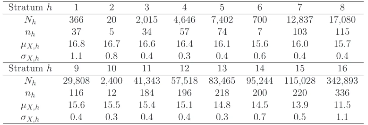
Table 3: The stratum size, sample allocation, mean and standard error of the inventory data on the log scale extracted from the 2014 Monthly Retail Trade Survey
Stratumh 1 2 3 4 5 6 7 8 Nh 366 20 2,015 4,646 7,402 700 12,837 17,080 nh 37 5 34 57 74 7 103 115 µX,h 16.8 16.7 16.6 16.4 16.1 15.6 16.0 15.7 σX,h 1.1 0.8 0.4 0.3 0.4 0.6 0.4 0.4 Stratumh 9 10 11 12 13 14 15 16 Nh 29,808 2,400 41,343 57,518 83,465 95,244 115,028 342,893 nh 116 12 184 196 218 200 220 336 µX,h 15.6 15.5 15.4 15.1 14.8 14.5 13.9 11.5 σX,h 0.4 0.3 0.4 0.4 0.3 0.7 0.5 1.1
6.2 Monthly retail trade survey
To demonstrate the practical relevance, we consider the U.S. Census Bureau’s 2014 Monthly Retail Trade Survey (Mulry et al.; 2014). The Monthly Retail Trade Survey is an economic indicator survey whose monthly estimates are inputs to the Gross Domestic Product estimates. This survey selects a sample of about12,000retail businesses each month with paid employees to collect data on sales and inventories. It employs an one-stage stratified sample with stratification based on major industry, further substratified by the estimated annual sales referred to as the size variable.
For simulation purpose, according to the 2014 Monthly Retail Trade Survey, we generate a finite population of N = 812,765 retail businesses with16 strata with a stratum identifier h, sales
Y, inventories X, and a size variable Z on the log scale. Table 3 reports some summary statistics extracted from the actual survey. We generate the inventory and size data fromXhi∼N(µX,h, σX,h2 ) andZhi∼N(µX,h, σ2X,h), fori= 1, . . . , Nhandh= 1, . . . ,16, and the sales data from a linear model
Yhi = β0+Xhi+Zhi+ǫhi, (14)
and a nonlinear model
Yhi =β0+ Xhi2 +Zhi2 +ǫhi, (15)
where ǫhi ∼ N(0,0.52). In (14) and (15), we specify different values forβ0 so that the parameter
of interest, µ=N−1P16h=1PNhi=1Yhi, matches with the true population mean 12.73.
We also generate a big data sample SB where the inclusion indicator δhi ∼Ber(phi) with the inclusion probability phi for unit iin stratumh. The big data sample in practice is often available from E-commercial companies who monitor inventories and sales for retail businesses. For the big data inclusion probability, we consider a logistic linear model
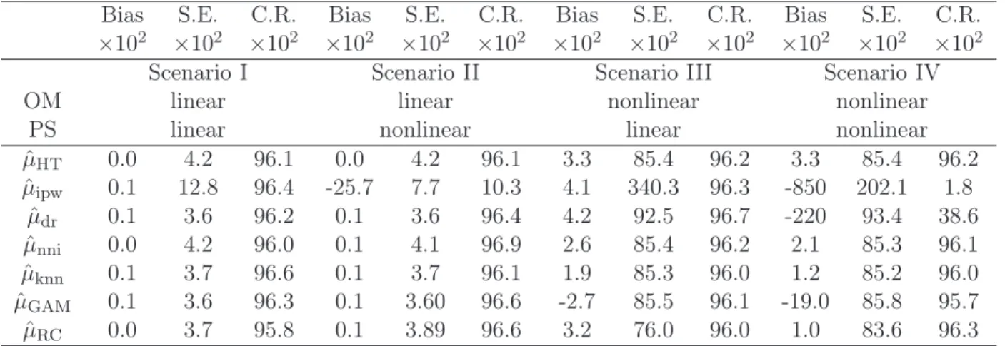
Table 4: Simulation results: bias, standard error, and coverage rate of 95% confidence intervals under four scenarios based on 1,000 Monte Carlo runs for the 2014 Monthly Retail Trade Survey. OM: outcome model; PS: propensity score model
Bias S.E. C.R. Bias S.E. C.R. Bias S.E. C.R. Bias S.E. C.R.
×102 ×102 ×102 ×102 ×102 ×102 ×102 ×102 ×102 ×102 ×102 ×102
Scenario I Scenario II Scenario III Scenario IV
OM linear linear nonlinear nonlinear
PS linear nonlinear linear nonlinear
ˆ µHT 0.0 4.2 96.1 0.0 4.2 96.1 3.3 85.4 96.2 3.3 85.4 96.2 ˆ µipw 0.1 12.8 96.4 -25.7 7.7 10.3 4.1 340.3 96.3 -850 202.1 1.8 ˆ µdr 0.1 3.6 96.2 0.1 3.6 96.4 4.2 92.5 96.7 -220 93.4 38.6 ˆ µnni 0.0 4.2 96.0 0.1 4.1 96.9 2.6 85.4 96.2 2.1 85.3 96.1 ˆ µknn 0.1 3.7 96.6 0.1 3.7 96.1 1.9 85.3 96.0 1.2 85.2 96.0 ˆ µGAM 0.1 3.6 96.3 0.1 3.60 96.6 -2.7 85.5 96.1 -19.0 85.8 95.7 ˆ µRC 0.0 3.7 95.8 0.1 3.89 96.6 3.2 76.0 96.0 1.0 83.6 96.3
and a nonlinear logistic model
logit(phi) =α0+Xhi+Zhi2, (17)
where we specify different values forα0so that the mean inclusion probability is about30%. Lastly,
we generate a representative sampleSAby stratified sampling with simple random sampling within strata without replacement; see Table 3 for the sample allocation.
We consider the seven estimators in§6.1 adopted for stratified sampling. In each mass imputed dataset, we apply the following point estimator and variance estimator: µˆ=N−1PHh=1Nhy¯nhwith
¯
ynh is the sample mean of y in the hth stratum, Vˆ(ˆµ) = N−2PhH=1Nh2(1−nh/Nh)s2nh/nh with
s2nh = (nh−1)−1Pinh=1(yhi−y¯nh)2.
Table 4 summarizes the simulation results. A similar discussion to§6.1 applies. µˆipw is sensitive
to misspecification of the selection model; whileµˆdr has double robustness feature, which still relies
on at least one model to be correctly specified. Mass imputation based on nearest neighbor im-putation, k nearest neighbor imputation and generalized additive model shows good performances by leveraging the representativeness of the survey sample and the predictive power of the big data sample. In addition, if the big data membership is known throughout the survey data, the regression calibration estimator gains efficiency while maintaining the robustness against model misspecifica-tion.
7
Discussion
Mass imputation is an important technique for survey data integration. When the training dataset for imputation is obtained from a probability sample, the theory of Kim and Rao (2012) can be directly applied. If the training dataset is a non-probability sample and its size is huge, we have shown in this article that various nonparametric methods can be used for mass imputation, and
the estimation error in the imputation model can be safely ignored, under the assumption that the sampling mechanism for training data is missing at random in the sense of Rubin (1976). If the sampling mechanism is believed to be not missing not at random, imputation techniques can be developed under the strong model assumptions for the sampling mechanism (e.g. Riddles et al.; 2016; Morikawa and Kim; 2018). Also, when the training dataset has a hierarchical structure, multi-level models can be used to develop mass imputation. This is closely related to unit-multi-level small area estimation in survey sampling (Rao and Molina; 2015). These are topics for future research.
Supplementary Material
Supplementary material includes the proofs for three theorems.
References
Abadie, A. and Imbens, G. W. (2006). Large sample properties of matching estimators for average treatment effects, Econometrica74: 235–267.
Baker, R., Brick, J. M., Bates, N. A., Battaglia, M., Couper, M. P., Dever, J. A., Gile, K. J. and Tourangeau, R. (2013). Summary report of the aapor task force on non-probability sampling, Journal of Survey Statistics and Methodology 1: 90–143.
Beretta, L. and Santaniello, A. (2016). Nearest neighbor imputation algorithms: a critical evalua-tion, BMC Med. Inform. Decis. Mak. 16: 198–208.
Breidt, F. J., McVey, A. and Fuller, W. A. (1996). Two-phase estimation by imputation, Journal of the Indian Society of Agricultural Statistics 49: 79–90.
Breidt, F. J. and Opsomer, J. D. (2017). Model-assisted survey estimation with modern prediction techniques, Statist. Sci.32: 190–205.
Cheng, P. E. (1994). Nonparametric estimation of mean functionals with data missing at random, Journal of the American Statistical Association 89: 81–87.
Chipperfield, J., Chessman, J. and Lim, R. (2012). Combining household surveys using mass imputation to estimate population totals,Australian & New Zealand Journal of Statistics54: 223– 238.
Deville, J.-C. and Särndal, C.-E. (1992). Calibration estimators in survey sampling, J. Am. Stat. Assoc. 87: 376–382.
Eilers, P. H. and Marx, B. D. (1996). Flexible smoothing with b-splines and penalties, Statistical Science 11: 89–102.
Hastie, T. and Tibshirani, R. (1990). Generalized Additive Models, NY: Chapman and Hall, Inc. Imbens, G., Johnson, P. and Spady, R. H. (1998). Information theoretic approaches to inference in
moment condition models, Econometrika66: 333–357.
Kalton, G. and Kish, L. (1984). Some efficient random imputation methods, Communications in Statistics-Theory and Methods 13: 1919–1939.
Keiding, N. and Louis, T. A. (2016). Perils and potentials of self-selected entry to epidemiological studies and surveys, Journal of the Royal Statistical Society: Series A (Statistics in Society) 179: 319–376.
Kim, J. K. and Fuller, W. (2004). Fractional hot deck imputation,Biometrika 91: 559–578. Kim, J. K. and Rao, J. N. K. (2012). Combining data from two independent surveys: a
model-assisted approach, Biometrika 99: 85–100.
Kitamura, Y. and Stutzer, M. (1997). An information-theoretic alternative to generalized method of moments estimation, Econometrica 65: 861–874.
Klenke, A. (2006). Probability Theory, Springer-Verlag: Heidelberg.
Mack, Y.-P. (1981). Local properties of k-NN regression estimates, SIAM Journal on Algebraic Discrete Methods 2: 311–323.
Mack, Y. and Rosenblatt, M. (1979). Multivariate k-nearest neighbor density estimates,Journal of Multivariate Analysis9: 1–15.
McCullagh, P. (1984). Generalized linear models, Eur. J. Oper. Res. 16: 285–292.
Morikawa, K. and Kim, J. K. (2018). A note on the equivalence of two semiparametric estimation methods for nonignorable nonresponse, Statistics & Probability Letters140: 1–6.
Mulry, M. H., Oliver, B. E. and Kaputa, S. J. (2014). Detecting and treating verified influential values in a Monthly Retail Trade Survey, J. Offic. Stat.30: 721–747.
Nelder, J. A. and Baker, R. J. (1972). Generalized Linear Models, Wiley Online Library.
Newey, W. K. and Smith, R. J. (2004). Higher order properties of GMM and generalized empirical likelihood estimators, Econometrica72: 219–255.
Park, M. and Fuller, W. A. (2012). Generalized regression estimators, Encyclopedia of Environ-metrics 2: 1162–1166.
Rao, J. N. and Molina, I. (2015). Small Area Estimation, Wiley: New York.
Riddles, M. K., Kim, J. K. and Im, J. (2016). A propensity-score-adjustment method for nonignor-able nonresponse, Journal of Survey Statistics and Methodology 4: 215–245.
Rivers, D. (2007). Sampling for web surveys,Joint Statistical Meetings. Rubin, D. B. (1976). Inference and missing data, Biometrika 63: 581–592.
Ruppert, D., Wand, M. P. and Carroll, R. J. (2009). Semiparametric regression during 2003–2007, Electronic Journal of Statistics3: 1193–1256.
Schennach, S. M. (2007). Point estimation with exponentially tilted empirical likelihood, Ann. Statist. 35: 634–672.
van der Vaart, A. W. (2000). Asymptotic Statistics, Cambridge University Press, Cambridge, MA. Wood, S. N. (2006).Generalized Additive Models: an Introduction with R, Chapman and Hall/CRC.
Supplementary material
by Shu Yang and Jae Kwang Kim
S1
Proofs
S1.1 Proof for Theorem 1
For a givenXi=xin Sample A, we show that Xi(1) converges to x in probability asNB→ ∞.To show this, consider for anyǫ >0,
P{d(Xi(1), x)> ǫ} = P{d(Xj, x)> ǫ ∀j∈B}
= [P{d(Xj, x)> ǫ}]NB. (S1)
By Assumption 2, x is in the support of X in Sample B. This leads to P{d(Xj, x) < ǫ} >0 and
P{d(Xj, x)> ǫ}<1. Therefore, (S1) converges to zero, andXi(1) converges tox in probability as
NB → ∞.
Given Xi =x, for any continuous and bounded g(y),
E{g(Yi(1))|Xi =x} = E[E{g(Yi(1))|Xi(1)} |Xi =x]
= E{µg(Xi(1))|Xi =x} → E{µg(Xi)|Xi=x}
= E{g(Yi)|Xi=x},
in probability asNB → ∞, where → follows from the fact that µg(x) is bounded and continuous. Then, by Portmanteau Lemma (Klenke; 2006), Yi(1) → Yi |(Xi =x) in distribution as NB → ∞. By Assumption 1, g(Yi(1)) |Xi → µg(Xi) +eg∗(Xi) in distribution as NB → ∞, where e∗g(Xi) has the same distribution as{g(Yi)|Xi} −µg(Xi).
We now show that for i6=j ∈A, e∗g(Xi) and e∗g(Xj) are conditionally independent, given data OA. It is sufficient to show that P{i(1) =j(1)} → 0 asNB → ∞; in other words, the same unit can not be matched for unit i and unit j with probability 1. This can be shown using (S1) with
ǫ= mini6=j∈A||Xi−Xj||.
Therefore, conditional on data OA,
ˆ µg,nni= 1 N X i∈A πi−1g(Yi(1))→ 1 N X i∈A πi−1g(Yi) = ˆµg,HT
Let ˜ Vnni= n N2 X i∈A X j∈A πij −πiπj πiπj g(Yi) πi g(Yj) πj . (S2)
Then, V˜nniis consistent forVnni.
Similar to the above argument, fori, j∈A, conditional on dataOA,g(Yi(1))g(Yj(1))→g(Yi)g(Yj) asNB → ∞. Therefore, conditional on dataOA,
ˆ Vnni= n N2 X i∈A X j∈A πij −πiπj πiπj g(Yi(1)) πi g(Yj(1)) πj → ˜ Vnni, (S3)
in distribution as NB→ ∞. Combining (S2) and (S3), Vˆnni is consistent for Vnni.
S1.2 Proof for Theorem 2
To investigate the asymptotic properties of µˆg,knn, we re-express
ˆ µg(x) = P j∈BKRx(x−Xj)g(Yj) P j∈BKRx(x−Xj) , where Kh(u) = 1 hpK u h , K(u) = 0.5I(||u|| ≤1),
and the bandwidth h =Rx is the random distance between x and its furthest among the k near-est neighbors. Therefore, µˆg,knn can be viewed as a kernel estimator incorporating a data-driven
bandwidth.
In the literature, asymptotic properties of theknearest neighbor imputation estimator have been studied extensively. The result shown in the following lemma on k nearest neighbor imputation is extracted from Mack (1981).
Lemma S1 Under Assumptions 1–3,
N−1 N X j=1 δB,jKRx(x−Xj)g(Yj) =f(x)πB(x)µg(x) +Op ( k N 2/p + 1 k ) . (S4) We now express ˆ µg,knn = 1 N N X i=1 πi−1δA,iµg(Xi) + 1 N N X i=1 π−i 1δA,i{µˆg(Xi)−µg(Xi)}.
Let TN = N−1PNi=1πi−1δA,i{µˆg(Xi)−µg(Xi)}. To study the properties for TN, we first look at
ˆ
µg(x), which can be expressed as
ˆ µg(x) =
hN(x)
fN(x)
where hN(x)≡N−1PNj=1δB,jKRx(x−Xj)g(Yj) andfN(x)≡N−1PNj=1δB,jKRx(x−Xj). By the result in Lemma S1, we obtain
hN(x) = f(x)πB(x)µg(x) +Op ( k N 2/p + 1 k ) fN(x) = f(x)πB(x) +Op ( k N 2/p + 1 k ) .
Now, by a Taylor expansion, we obtain
ˆ µg(x)−µg(x) = hN(x) fN(x) − µg(x) = 1 f(x)πB(x){ hN(x)−f(x)πB(x)µg(x)} −f(x)πB(x)µg(x) {f(x)πB(x)}2 { fN(x)−f(x)πB(x)}+Op ( k N 2/p + 1 k ) = 1 f(x)πB(x){ hN(x)−fN(x)µg(x)}+Op ( k N 2/p + 1 k ) . Therefore, we obtain TN = 1 N2 N X i=1 δA,i πi 1 f(Xi)πB(Xi) N X j=1 δB,jKRXi(Xi−Xj){g(Yj)−µg(Xi)}+Op ( k N 2/p + 1 k ) .
Under the assumption in Theorem 2, it is easy to drive that (k/N)2/p+ 1/k = o(n−1/2), and therefore, TN = 1 N2 N X i=1 δA,i πi 1 f(Xi)πB(Xi) N X j=1 δB,jKRXi(Xi−Xj){g(Yj)−µg(Xi)}+op(n−1/2).
We then express TN in a form of U-statistics (van der Vaart; 2000; Ch. 12):
TN = 1 N(N −1) N X i=1 X j6=i h(Zi, Zj) +op(n−1/2),
where Zi = (Xi, Yi, δA,i, δB,i) and
h(Zi, Zj) = 1 2 δA,iδB,j πi 1 f(Xi)πB(Xi) KRXi(Xi−Xj){g(Yj)−µg(Xi)} + δA,jδB,i πj 1 f(Xj)πB(Xj) KRXj(Xj−Xi){g(Yi)−µg(Xj)} ≡ 12(ζij +ζji).
Now, by Lemma S1, we obtain E(ζij |Zi) = E δ A,iδB,j πi 1 f(Xi)πB(Xi) KRXi(Xi−Xj){g(Yj)−µg(Xi)} |Zi = δA,i πi 1 f(Xi)πB(Xi) EhδB,jKRXi(Xi−Xj){g(Yj)−µg(Xi)} |Zi i = O ( k N 2/p +1 k ) , and E(ζji|Zi) = E δA,jδB,i πj 1 f(Xj)πB(Xj) KRXj(Xj −Xi){g(Yi)−µg(Xj)} |Zi = δB,iE E δA,j πj 1 f(Xj)πB(Xj) KRXj(Xj−Xi){g(Yi)−µg(Xj)} |RXj, Zi |Zi = δB,i πB(Xi){ g(Yi)−µg(Xi)}+O ( k N 2/p + 1 k ) .
Therefore, by the theory of U-statistics, we obtain
TN = 2 N N X i=1 E{h(Zi, Zj)|Zi}+op(n−1/2) = 1 N N X i=1 δB,i πB(Xi){ g(Yi)−µg(Xi)}+op(n−1/2).
Combining the above results leads to
ˆ µg,knn−µg = 1 N N X i=1 πi−1δA,iµg(Xi)−µg(Xi) +1 N N X i=1 δ B,i πB(Xi) − 1 {g(Yi)−µg(Xi)}+op(n−1/2). (S5) Then, the asymptotic results in Theorem 2 follow by Assumptions 1–4 and (S5).
S1.3 Proof for Theorem 3
The consistency and asymptotic normality of n1/2µˆg,nni follow by the standard arguments under
Assumptions 1–4. The remaining is to show that the asymptotic variance of n1/2µˆg,nni is Vnni.
leads to generalized regression estimation (Park and Fuller; 2012). Therefore, we express n1/2µˆg = n 1/2 N X i∈A ωig(Yi(1)) = n 1/2 N X i∈A π−i 1g(Yi(1))−n 1/2 N X i∈A π−i 1hT iβN− N X i=1 hT iβN ! +op(n−1/2). (S6)
Similar to the argument in the proof for Theorem 1, we express
n1/2µˆg = n1/2 N X i∈A πi−1g(Yi(1))−n 1/2 N X i∈A πi−1hT iβN − N X i=1 hT iβN ! +op(n−1/2) = n 1/2 N X i∈A πi−1g(Yi(1))−hTiβN +n 1/2 N N X i=1 hT iβN +op(n−1/2). (S7)
It is straightforward to show the variance of the second term in (S7) is negligible givennN−1=o(1). Following the arguments in the proof for Theorems 1 and 2,g(Yi(1))has the asymptotic distribution
asg(Yi) given the data OAfrom Sample A. Therefore, the asymptotic variance of n1/2µˆg is
VRC = lim n→∞var " n1/2 N X i∈A πi−1{g(Yi)−hTiβN} # .