Investigating different levels of joining entity and relation classification

(1)

Institute for Natural Language Processing University of Stuttgart

Pfaffenwaldring 5B D–70569 Stuttgart

Bachelorarbeit

Investigating Different Levels of

Joining Entity and Relation

Classification

Milan Milovanovic

Course of Study: Informatik

Examiner: Prof. Dr. Sebastian Padó, Dr. Roman Klinger

Supervisor: Heike Adel

Commenced: April 4, 2018

(2)

Abstract

Named entities, such as persons or locations, are crucial bearers of infor-mation within an unstructured text. Recognition and classification of these (named) entities is an essential part of information extraction. Relation clas-sification, the process of categorizing semantic relations between two entities within a text, is another task closely linked to named entities. Those two tasks – entity and relation classification – have been commonly treated as a pipeline of two separate models. While this separation simplifies the problem, it also disregards underlying dependencies and connections between the two subtasks. As a consequence, merging both subtasks into one joint model for entity and relation classification is the next logical step.

A thorough investigation and comparison of different levels of joining the two tasks is the goal of this thesis. This thesis will accomplish the objective by defining different levels of joint entity and relation classification and develop-ing (implementdevelop-ing and evaluatdevelop-ing) and analyzdevelop-ing machine learndevelop-ing models for each level. The levels which will be investigated are:

• (L1) a pipeline of independent models for entity classification and re-lation classification

• (L2) using the entity class predictions as features for relation classifi-cation

• (L3) global features for both entity and relation classification

• (L4) explicit utilization of a single joint model for entity and relation classification

The best results are achieved using the model for level 3 with an F1 score of

(3)

Kurzfassung

Entitäten, wie Personen oder Orte sind ausschlaggebende Informationsträger in unstrukturierten Texten. Das Erkennen und das Klassifizieren dieser En-titäten ist eine entscheidende Aufgabe in der Informationsextraktion. Das Klassifizieren von semantischen Relationen zwischen zwei Entitäten in einem Text ist eine weitere Aufgabe, die eng mit Entitäten verbunden ist. Diese zwei Aufgaben (Entitäts- und Relationsklassifikation) werden üblicherweise in einer Pipeline hintereinander mit zwei verschiedenen Modellen durchge-führt. Während die Aufteilung der beiden Probleme den Klassifizierungspro-zess vereinfacht, ignoriert sie aber auch darunterliegende Abhängigkeiten und Zusammenhänge zwischen den beiden Aufgaben. Daher scheint es ratsam, ein gemeinsames Modell für beide Probleme zu entwickeln.

Eine umfassende Untersuchung von verschiedenen Stufen der Verknüpfung der beiden Aufgaben ist das Ziel dieser Bachelorarbeit. Dazu werden Modelle für die unterschiedlichen Stufen der Verknüpfung zwischen Entitäts- und Re-lationsklassifikation definiert und mittels maschinellen Lernens ausgewertet und evaluiert. Die verschiedenen Stufen die betrachtet werden, sind:

• (L1) Verwendung einer Pipeline zum sequentiellen und unabh¨angigen Ausf¨uhren beider Modelle

• (L2) Verwendung der Vorhersagen über die Entitätsklassen als Merk-male für die Relationsklassifikation

• (L3) Verwendung von globalen Merkmale f¨ur sowohl die Entit¨ atsklassi-fikation als auch f¨ur die Relationsklassifikation

• (L4) Explizite Verwendung eines gemeinsamen Modells zur Entit¨ ats-und Relationsklassifikation

Die besten Resultate wurden mit dem Modell f¨ur Level 3 erreicht. Das F1

-Maß der Entit¨atsklassifikation betr¨agt 0.830 und das F1-Maß der

(4)

1 Introduction

Information Extraction (IE) describes the process of taking unstructured text as input and creating structured and unambiguous data as output. This usually requires a text processing task to identify and recognize necessary information, such as named entities and relations among them. Named en-tities include many different types of words such as locations, persons or organisations. Named entity recognition and classification is defined as the task of detecting and classifying named entities in an unstructured text. Several learning methods using diverse classifiers for supervised learning or more uncommon unsupervised learning are in use (McCallum and Li, 2003). The recognition and classification of named entities is a necessity to extract relations between two or more entities from a sentence. Relations typically include physical relations (located etc.) or social relations (family, employ-ment etc.) among others (Wang et al., 2006). As the extraction of relations is based on the recognition and classification of entities, the two tasks have been commonly treated as a pipeline of two independent models (Miwa and Sasaki, 2014). While this separation simplifies the task, it also disregards un-derlying dependencies and connections between the two subtasks (Miwa and Sasaki, 2014). The model is prone to error propagation due to the pipeline approach as errors in entity recognition are propagated downwards to relation extraction. Furthermore, the model does not consider cross-task dependen-cies. Thus, a combination of both subtasks into one joint model seems like the next logical step (Li and Ji, 2014).

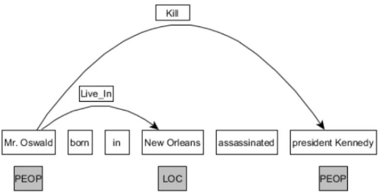
Figure 1 shows a visualization of a sentence with already annotated named entities and relations. A Kill relation requires two People entities and a Live In relation requires People and Loc entities. The task of extracting re-lations is not possible without recognition and classification of the required named entities.

(7)

Figure 1: An example of entity and relation. Named entities persons (Peop) and locations (Loc) are connected by relations Kill and Live In (Roth and Yih, 2004).

1.1 Goal of the Thesis

The purpose of this thesis is therefore to investigate different levels of joining entity and relation classification by examining the results for each level. The dataset used for this thesis is the ”entity and relation recognition” (ERR) dataset from (Roth and Yih, 2004). The models for each level have a gradi-ent increase of joining the two subtasks by using an incremgradi-ental amount of cross-task features per level similar to (Li and Ji, 2014). Level one to three use a linear-chain conditional random field (CRF) as introduced by Lafferty et al. (2001) for entity classification while understanding the task of relation extraction as a multi-class classification problem (Zhou et al., 2005). The extraction of relations can be understood as the process of finding the nec-essary named entities and using a pair of entities as model input for relation classification. Given an entity pair {e1, e2} the classification method has to decide what relation (if any) exists between the given pair (Roth and Yih, 2004; Zhou et al., 2005).

While level one uses the pipeline model of two independent subtasks, level two increases the level of joining entity and relation classification by using

(8)

en-tity type information for relation extraction similar to Giuliano et al. (2007). Furthermore, level three uses relation type features for entity classification while keeping all other features. The model utilized for level four uses a single joint model for entity and relation classification similar to the one described by (Zheng et al., 2017).

The main research question investigated in this thesis is

• Which level or joining entity and relation classification performs the best?

This can be further divided into the following sub-questions:

• Which model performs the best?

• Which features are key to the performance?

Structure of the Thesis

This thesis is structured in the following manner:

Chapter 1-Introduction:The topic and goals of the thesis are introduced. Chapter 2 - Related Work: Related work is introduced.

Chapter 3 -Background:The fundamentals needed for named entity and relation classification are explained. This includes the principles of evaluation metrics and the definition of classification methods.

Chapter 4 -Data:This chapter focuses on the data and necessary prepro-cessing steps.

Chapter 5 - Models: The models, features and hyperparameters used for this thesis are introduced and specified.

Chapter 6-Results and Analysis:The experiments and their results will be presented and analysed.

Chapter 7 -Conclusion and Future Work:The main findings are sum-marized and possible directions for future works are identified.

(9)

2 Related Work

The two tasks, entity and relation classification, have had multiple proposed models over the past years. A very popular model is the pipeline approach of treating the two tasks as a pipeline of two independent models. Other models use end-to-end methods to join entity and relation classification. A special focus will be put on works and studies using the same dataset as this thesis.

Traditional methods to handle this task is a pipeline manner, recognizing the entities first and then extracting their relations (Zheng et al., 2017). Most existing named entity recognition models use linear-chain conditional random fields (CRF) whose performances heavily rely on annotated features extracted by NLP tools (Wang et al., 2006; Lafferty et al., 2001; Yao et al., 2009). Florian et al. (2003) present a classifier-combination framework for named entity recognition using gazetteer information as features. The tradi-tional models used for relation classification largely rely on feature represen-tation (Kambhatla, 2004) or kernel design (Zelenko et al., 2003). Recently new models using neural networks have been proposed to both tasks with great success such as the combination of bidirectional LSTMs and conditional random fields by Lample et al. (2016) for named entity recognition and the introduction of dependency-based neural networks for relation classification by Liu et al. (2015).

Multiple studies and works use the ”entity and relation recognition” (ERR) dataset (Roth and Yih, 2004; 2007) although with different models. Roth and Yih (2004) use linear programming with constraints to normalize en-tity types and relations on a global scale. In contrast to the typically used pipeline framework, this model does not trust the results of classification and is therefore able to overcome mistakes made by classifiers with the us-age of constraints (Roth and Yih, 2004). Kate and Mooney (2010) describe a novel method for joint entity and relation extracting by using a card-pyramid

(10)

graph which encodes all possible entities and relations in a sentence, reducing the task of their joint extraction to jointly labeling its nodes. Giuliano et al. (2007) use entity type information for relation extraction without training both tasks in a joint model. Furthermore, Giuliano et al. (2007) use a com-bination of kernel functions to integrate two different information sources which include the whole sentence where the relation appears and the local contexts around the entities participating in the relation. The results of re-lation extraction show that the novel approach of using entity type informa-tion as features for relainforma-tion extracinforma-tion, significantly improves previous results achieved on the same dataset (Giuliano et al., 2007). Miwa and Sasaki (2014) propose a novel learning approach that jointly extracts entities and relations of a sentence by introducing a flexible table representation of entities and relations. The task of entity and relation classification is then mapped to a simple table-filling problem which outperforms the pipeline approach. Adel and Sch¨utze (2017) note that previous works also use a variety of linguistic features, such as part-of-speech tags. Other works not using the ERR dataset include a single probabilistic graphical system for both tasks (Singh et al., 2013) and a model to incrementally join entity and relation extraction using structured perceptron with efficient beam-search (Li and Ji, 2014). Li and Ji (2014) assess that the results of entity recognition affect the performance of relation classification. Zheng et al. (2017) introduce a novel tagging scheme converting the task of joining entity and relation extraction to a tagging problem.

Similar to Roth and Yih (2004), Kate and Mooney (2010) and Giuliano et al. (2007) the models used for level one to three train separate models for entity and relation classification on the dataset while understanding the task of relation extraction as the task of identifying relations between named entity pairs. Thus, the query entities for relation extraction are only named entity pairs.

(11)

The features for the models used for named entity recognition and classi-fication are similar to the features used by Florian et al. (2003) and Miwa and Sasaki (2014) and includes annotated features such as part-of-speech tags, word types and surrounding words. Some features are more general and the gazetteer information is excluded. Features for relation extraction include the usage of shortest dependency paths and their length similar to Xu et al. (2015) and context information such as the sentence the query entity pairs appear in. The model for level two also uses entity type information as features for relation extraction as introduced by Giuliano et al. (2007). The model for level three uses global features similar to Miwa and Sasaki (2014). The model for level four uses a similar tagging scheme as Zheng et al. (2017) with the inclusion of adjacency nodes in the dependency graph as features.

In contrast to most works, the goal of this thesis is the investigation of differ-ent levels of joining differ-entity and relation classification. Miwa and Sasaki (2014) compare two different levels of joining both tasks while this thesis defines and investigates four different levels of joining entity and relation classification. Thus, the usage of features has to be constant across all levels with the in-cremental increase of cross-task features that help evaluating the process of finding out which level of joining the both tasks leads to the best result.

(12)

3 Background

3.1 Evaluation Metrics

The metric chosen for evaluation is very decisive. The selection of metrics influences how the performance of machine learning algorithms is measured and compared. The focus on different weights of characteristics is dependent on the choice of the evaluation metrics. Accuracy, Precision-Recall, F1 score

and confusion matrices are common options when deciding for a classification metric (Hossin and Sulaiman, 2015).

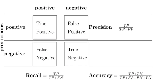
Precision and recall are classification metrics used to evaluate systems. Pre-cision is the percentage of relevant answers in the result and recall is the percentage of relevant answers that have been predicted (Kent et al., 1955). In binary classification, a classifier labels documents as either positive or neg-ative. This decision can be represented in a so called confusion matrix (or contingency table). The four categories of the table are the following: True positives (TP), false positives (FP), false negatives (FN) and true negatives (TN). True positives are positives which have been correctly labeled as posi-tives. Likewise, true negatives are negatives which have been correctly labeled as negatives. False positives and false negatives however have an incorrect label. While false positives refer to negatives that have been wrongly labeled as positives, false negatives are positives that have been incorrectly labeled as negatives.

Table 1 shows the confusion matrix and the definitions of precision and recall where TP, FP and FN denote the number of true positives, false positives and false negatives, respectively.

(13)

predictions gold values positive negative positive True Positive False Positive Precision= T P T P+F P negative False Negative True Negative Recall= _{T P}T P₊_{F N} Accuracy= _{T P}₊_{F P}T P₊+_{F N}T N₊_{T N} Table 1: Confusion matrix

The standard way to combine precision and recall into one single performance measure is through the F1 score. The F1 score is the harmonic average of

precision and recall. It reaches its best value at 1 and its worst score at 0. (1) F1 = 2 1 precision + 1 recall = 2·precision·recall precision + recall = TP TP + FP + FN 2

Two different methods are commonly used to determine the average; Micro-and macro average. Micro- Micro-and macro-averages are computed slightly dif-ferently and thus their interpretation differs. A macro-average computes the metric independently for each label and then takes the average. It treats all classes equally. Whereas a micro-average tries to aggregate the contributions of all classes to compute the average metric. The micro-average is affected less by performance on rare labels. Thus, it is preferable to use the micro-average in a multi-label classification problem (Lipton, Zachary Chase and Elkan, Charles and Narayanaswamy, Balakrishnan, 2014). The two methods can both be applied to both evaluation metrics, PR and F1 score.

(14)

3.2 Part-of-Speech

Part-of-speech tagging is the assignment of words and punctuation characters of a text to their corresponding part-of-speech label. A part of speech is a category of lexical items with similar properties Brill (1992). A list of part-of-speech tags can be found in the appendix (Figure 11).

3.3 Training, Test and Validation Sets

One of the core concepts of machine learning is the notion of creating a model, capable of accurately making predictions on test data. Machine learning mod-els need information to precisely make predictions. The training set is used to give the necessary information to the models (train) while the test set, like the name implies, is used for testing. The test set is untouched during training and only used in the end for testing and analysing the generalisability of the model. A third set needs to be prepared to estimate the prediction error for model selection, the validation set or development set (Guyon, 1997). While performing machine learning the following steps are advised: Initially the gold data is utilized to train the model by pairing the input with the expected output. Then in order to estimate how well the model has been trained and to adjust model properties (to find optimal numbers) a validation set is used (Hastie, Trevor and Tibshirani, Robert and Friedman, Jerome, 2001). Lastly a test set is utilized to assess the performance of a trained model and to en-sure unbiased classification. Tuning the model after assessing the model on the test set is not advised as it leads to an underestimation of the true test er-ror and is prone to biased decisions. Using cross-validation or a validation set may give an overall insight on how the model will predict a completely new dataset (Hastie, Trevor and Tibshirani, Robert and Friedman, Jerome, 2001).

As a general rule a typical split might be 50% for training, and 25% each for validation and testing (Hastie, Trevor and Tibshirani, Robert and Friedman, Jerome, 2001). Determining what fraction of the data set should be reserved

(15)

as a validation set is a controversial topic as optimal performance depends on various factors (Guyon, 1997). This thesis uses a 60%−20%−20% split of the training, validation and test set (see Section 4).

3.4 N-Gram

N-Grams are the results of partitioning a given text into fragments. An n-gram is a contiguous sequence of n characters or words of a given sample. An n-gram size of n = 1 is called unigram, size 2 is called bigram and an n-gram of size 3 is a trigram (Hastie, Trevor and Tibshirani, Robert and Friedman, Jerome, 2001). Sometimes the beginning and end of a text are explicity modeled to match beginning-of-word and ending-of-word situations (Cavnar, William B and Trenkle, John M and others, 1994) and a special character (e.g. ” ”) is used to represent blanks. Therefore the word ”Word” has the following character:

• unigrams: , W, O, R, D,

• bigrams: W, WO, OR, RD, D

• trigrams: WO, WOR, ORD, RD , D

3.5 Vector Space Model and Bag-of-Words Model

Vector space model as introduced by Salton et al. (1975) is an algebraic model for representing a set of documents as vectors in a common vector space. As raw data (a sequence of characters) cannot be put into algorithms because they expect numerical features, the text documents have to undergo a vectorization process. In general this describes the process of turning a col-lection of text documents into numerical feature vectors (Ko, 2012). In the vector space model, a document is represented as a vector d= (w1, ..., w|V|),

(16)

term w1 represents how much the term w1 contributes to the semantics of

the document d (Ko, 2012). The term weight may be a binary value (with 1 indicating that the term occured in the document, and 0 indicating that it did not occur in the document) or a term frequency value tft,d (equal to

the number of occurrences of term t in the document d) among others. The model of only counting the occurrences of each term but ignoring their rel-ative position information in the document is called the bag-of-words model (Sch¨utze et al., 2008). Thus, the documents d1 = ”John likes Mary” and

d2 = ”Mary likes John” appear the same in this model. As term frequency is

not necessarily the best representation for a text due to common words like ”the” or ”a” being almost always among the highest frequency terms in the text, the utilization of stop words is recommended (Tsz-Wai Lo et al., 2005).

3.6 Encoding with BILOU

The task of named entity recognition is commonly viewed as a prediction problem with the aim to assign the correct label for each token. There are many different ways of encoding information into a set of labels. This leads to many different representations of chunks. Two frequently used schemes are BILOU and BIO (Ratinov and Roth, 2009).

BIO stands for (B)eginning, (I)nside and (O)utside encoding of a text seg-ment. Beginning signifies the beginning of a named entity. Inside signifies that the word is inside a named entity and outside signifies that the word is just a regular word outside of a named entity. Below is a sample sentence annotated in BIO:

• Tuvia Tzafir is from Israel

• B-Person I-Person O O B-Location

In BIO encoding labels can either be the beginning of an entity (B X) or the continuation of an entity (I X).

(17)

BILOUencodes the (B)eginning, the (I)nside and the (L)ast token of multi-token entities while (U)nit multi-tokens are separated from other entities. (O)utside still signifies regular words not in a named entity. The same sentence is dif-ferently annotated in BILOU:

• Tuvia Tzafir is from Israel

• B-Person L-Person O O U-Location

In BILOU encoding, I X can only follow B X and L X can either follow B X or I X. Ratinov and Roth (2009) have shown that for some datasets, BILOU outperforms BIO.

3.7 Classification

In text classification, a fixed set of classes C ={c1, c2, ..., cn}and an amount

of inputs (which can be documents, sentences or words, depending on the task)d ∈X is given. Classes can also be called categories or labels. A prime example of classes are spam or non-spam emails. Furthermore a training set

D of labeled inputs is given where each input hd, ci, where hd, ci ∈ X ×C

(e.g. hd, ci=hJ ohn F. Kennedy, P erson i).

Using a learning method, we then wish to learn a classifierfthat maps inputs to their label: f : X → C (Sch¨utze et al., 2008). This is called supervised learning. Supervised learning can be seen as a function y = f(x) where y

needs to be predicted, x is the data while f is a function that needs to be learned. In short, supervised learning describes the process (given an already known training set of correctly labeled documents) of identifying to which set of categories a new document belongs to.

This process can be enhanced by using features. Features (or attributes) are representing characteristics of the input. Features for text classification

(18)

may include the frequency of specific terms or the amount of punctuation characters. Features for named entity recognition usually include lexical fea-tures such as word types (lowercase, pos-tags etc.) or contextual feafea-tures like surrounding words or variables indicating the position of the word in the sentence. Section 5.6 shows the features used for this thesis. Features also need to be turned into a vector model as classifiers need numerical features to represent a document.

In the following sections the classifiers used for this thesis will be presented.

3.7.1 Support Vector Machine

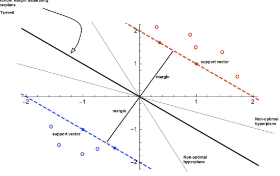
A Support Vector Machine (SVM) is a classifier defined by a separating max-margin hyperplane. Given already labeled training data, the algorithm tries to create an optimal hyperplane to categorize new examples. In two-dimensional space the hyperplane is a line and in three-two-dimensional space it is an ordinary plane. A vector w is defined as a weight vector which is perpendicular to the hyperplane and an intercept term b is defined. All points x on the hyperplane satisfy: wT_x₊_b _{= 0. Quadratic optimization}

can be used to find the plane. In a binary classification problem the two classes are yi = +1 and yi = −1. The linear classifier is then defined as

f(x) =sign(wT_x₊_b_{) where the sign indicates the class. As multiple}

hyper-planes exist the hyperplane with the highest margin should be selected as it guarantees the best generalisability (Sch¨utze et al., 2008). Figure 2 shows the maximum-margin separating hyperplane in a simple two-dimensional binary classification problem. The margin is maximized for all points on the selected hyperplane. Non-optimal hyperplanes do not satisfy this requirement.

3.7.2 Perceptron

The perceptron is an algorithm used to classify binary data. The perceptron algorithm learns to separate data by changing weights w and bias b using

(19)

Figure 2: Example of a hyperplane.

iteration. A variable 0 < α≤1 is defined as the learning rate, which indicates how quickly the algorithm responds to changes. The functionf is defined as:

f(x) =    1 if wT_x₊_{b >}₀ 0 otherwise Perceptron follows an update rule:

1. Perform the following steps for all inputs xi for each example i in the

training set where fi is the predicted output and di is the desired

out-put. Two classes are defined as di = 1 if xi belongs to that class and

di = 0 otherwise.

2. Initializing the algorithm with w(0), b(0), t= 0

2a. Calculate the output by computing the dot product:

(20)

2b. Update the weights and bias accordingly for the next iteration:

wi(t+ 1) =wi(t) +α(di −fi(t))xi

b(t+ 1) =b(t) +α(di−fi(t))

t=t+ 1

The perceptron is guaranteed to converge if the training set is linearly sep-arable (Collins, 2002). The perceptron can naturally be generalized to learn and classify multiclass classification problems. (Collins, 2002).

3.7.3 Decision Tree Classification

Decision Trees are a supervised learning method used for classification. The Decision Tree Classification uses decision trees to create a model that makes predictions by learning simple decision rules inferred from data features. In the context of named entity recognition, asked questions may include ”Is the word in lowercase?” among others. The decision tree classifier asks questions with the highest information gain first aiming to reduce uncertainty.

3.7.4 Logistic Regression

Logistic regression, also known as Maximum Entropy (Manning and Klein, 2003), is a statistical model used to estimate probabilities. At the core of the method lies the logistic function 1/(1 +eX_{). Input values} _x

i are combined

using weights (coefficients) w to predict a score:

score(xi, k) =w0,k+w1,kx1,i+...+wN,kxN,i=wk·xi

In machine learning, logistic regression is a widely used method with the goal to model the probability of a random variable y being 0 or 1:

(2) p(y|x) =    hθ(x) if y= 1 1−hθ(x) if y= 0

(21)

where θ is the set of weights w (θ is the vector of weights) and hθ(x) =

1

1 +e−θT_X =P r(Y = 1|X;θ)

The probability function can be written as:

(3) p(y|x) = (hθ(x))y(1−hθ(x))1−y

Using the maximum log-likelihood forN observation to estimate parameters:

l(θ|x) = log[ N Y n=1 (hθ(xn))yn(1−hθ(xn))1−yn] (4) l(θ|x) = N X n=1 [ynloghθ(xn) + (1−yn) log(1−hθ(xn))] (5)

While logistic regression is a probabilistic model for binomial cases, it can easily be extended for multinomial cases (multinomial logistic regression):

(6) p(y|x) =                        exp(θT 1x) PN i=1exp(θ T i x) if y = 1 exp(θT 2x) PN i=1exp(θTi x) if y = 2 . . . exp(θ_NTx) PN i=1exp(θTi x) if y =N

The following steps are omitted as they are corresponding to the binomial model. Unlike Naive Bayes Classifiers, Maximum Entropy does not assume statistical independence of features. In short, the logistic regression classifier computes the posterior class probability of an example by evaluating the normalized product of the active weights (Florian et al., 2003).

3.7.5 Conditional Random Field

A Conditional Random Field (CRF) is a method used for structured predic-tion. A Linear-Chain CRF is a special form of a CRF with linear structure

(22)

(mainly used in natural language processing) used to predict sequences of labels for sequences of input samples. In a linear-chain CRF for text process-ing, each feature function fi is a function that takes as input: The sentence

s, the positioni of a word in the sentence s, the labelli of the current word

and the label li−1 of the previous word (Lafferty et al., 2001). Assigning a

weight λj (finding the value of the weight by e.g. gradient descent) to each

feature functionfj allows to score a labeling lofsby adding up the weighted

features over all words in the sentence:

(7) score(l|s) = m X j=1 n X i=1 λjfj(s, i, li, li−1)

Where n is the amount of words in the sentence and m is the amount of sentences in the data. Transform the scores into probabilities p(l|s) between 0 and 1: (8) p(l|s) = Pexp[score(l|s)] l0exp[score(l0|s)] = exp[ Pm j=1 Pn i=1λjfj(s, i, li, li−1)] P l0exp[ Pm j=1 Pn i=1λjfj(s, i, li0, l 0 i−1)]

The formula only includes features for the current and previous word’s iden-tity. Extending the linear-chain formula to include richer features such as prefixes and suffixes of the current word and the identities of surrounding words is fortunately very simple as the definition is quite extensible (Sutton et al., 2012).

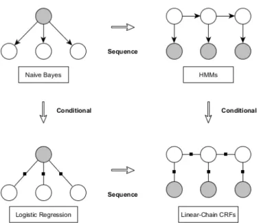
Equation 8 is similar to the ones used in logistic regression as CRFs are basically the sequential version of logistic regression (Sutton et al., 2012). Figure 3 shows the relationship of naive bayes, logistic regression, hidden markov models (HMMs) and linear-chain CRFs. The also shown HMMs are another possible sequence model which is not used in this thesis.

(23)

Figure 3: Relationships between Naive Bayes, Logistic Regression, HMMs and Linear-Chain CRFs (Sutton et al., 2012)

3.7.6 Stochastic Gradient Descent Classifier

Stochastic Gradient Descent (SGD) is a simple stochastic approximation of the gradient descent optimization method for minimizing a function. SGD tries to find minima (or maxima) by iteration. Hence, the SGD Classifier is a linear classifier that uses SGD for training by looking for the minima of the loss function using SGD. The loss function may be linear SVMs or logistic regression.

3.8 Dependency Grammar

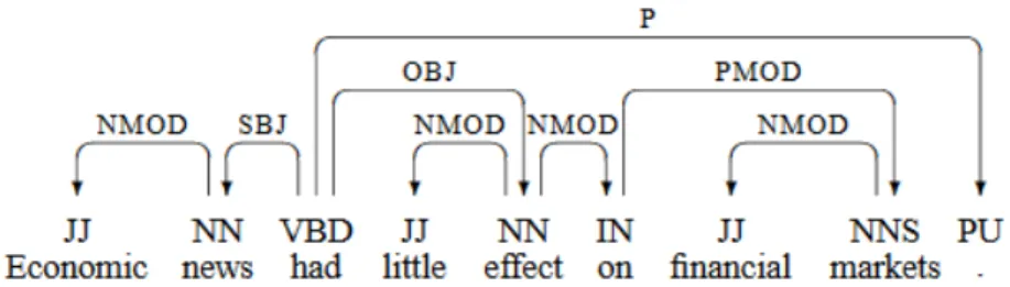
In dependency grammars the syntactic structure of a sentence is described by the words in a sentence and an associated set of grammatical relations. Unlike phrase structure grammar, dependency grammar only focuses on how words relate to other words.

(24)

Figure 4: Dependency structure for an English sentence from the Penn Tree-bank (Kubler et al., 2009): Arrows point from heads to their dependents while labels indicate the grammatical function of the word as either subject or object.

(25)

4 Data

CoNLL (Conference Computational Natural Language Learning) is a con-ference organized by the SIGNLL (ACL’s Special Interest Group on Natural Language Learning). The Text REtrieval Conference (TREC) is a series of conferences focusing on different information retrieval topics and research areas. The dataset which will be used for the experiments and analysis of this thesis is the ”Entity and Relation Recognition” dataset1_{. It consists of}

5516 sentences from the TREC corpus which have been manually annotated with four entity types and relations between them (Roth and Yih, 2004).

4.1 Structure of the Data

The data is split into a block for each sentence. Each block contains infor-mation about the entities and relations of one sentence. The format of each block is the following:

• the sentence and all the other columns in a table model

• empty line

• relation assignments (may be empty if no relations exist in the sentence)

• empty line

It is certainly possible for a sentence in the dataset to not contain any re-lations. When this is the case, the relation descriptors are omitted as they serve no purpose. It is also possible for a sentence to have more than one relation. The additional relations are simply added below.

In the block, each row represents an element (a single word, consecutive words or punctuation characters) of the sentence. The columns hold different amounts of expressiveness. The columns contain the following information:

1

(26)

• Column 1: SentenceID (sentence order number)

• Column 2: (Named) Entity class label

• Column 3: TokenID (The order of the elements in the sentence)

• Column 4: O

• Column 5: Part-of-speech tags

• Column 6: Tokens (words or punctuation characters)

• Column 7: O

• Column 8: O

• Column 9: O

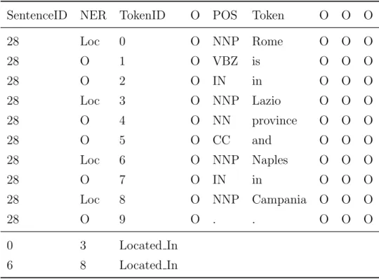
As shown in the enumeration afore, the only columns to contain valuable information are columns one to three, five and six. All other columns can simply be ignored. Table 2 shows an exemplary sentence with relations in the dataset.

Four named entities are given in the CoNLL-2004 dataset: Location, Or-ganisation, People and Other. Likewise, five relations are given in the CoNLL-2004 dataset:Located In,Work For,OrgBased In,Live Inand Kill. The entity-relation dependencies are defined as shown in Table 3. There are no other possible relations other than those shown in the table. It is pos-sible that a single named entity participates in more than one relation. It is however not possible that a single relation includes more (or less) than two named entities. Relations between eponymous entity types are reasonable except for the entity type Organisation. Relations are directed and are not reversible. Thus, a Person named Mike is able to live in Rome, Rome is not able to live in a Person named Mike.

(27)

SentenceID NER TokenID O POS Token O O O 28 Loc 0 O NNP Rome O O O 28 O 1 O VBZ is O O O 28 O 2 O IN in O O O 28 Loc 3 O NNP Lazio O O O 28 O 4 O NN province O O O 28 O 5 O CC and O O O 28 Loc 6 O NNP Naples O O O 28 O 7 O IN in O O O 28 Loc 8 O NNP Campania O O O 28 O 9 O . . O O O 0 3 Located In 6 8 Located In

Table 2: Example of a sentence with relations

4.2 Data Preprocessing

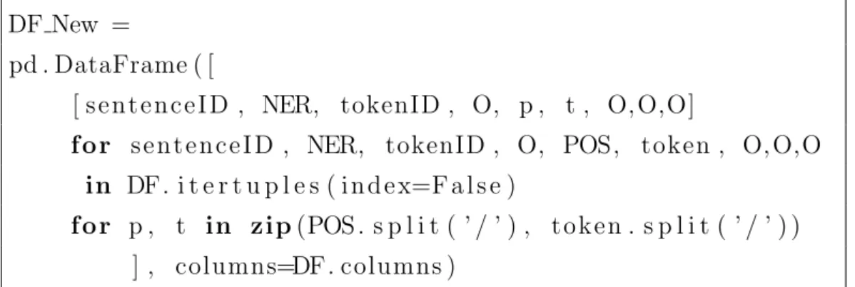
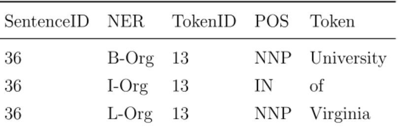
As the data is already annotated there is almost no need to revise it. It is how-ever necessary to split multi-token entities (Table 4) into single tokens to get them into the BILOU encoding scheme (Table 5). Splitting multi-token enti-ties is done by splitting on a special character. Most special characters such as brackets or parentheses are for instance replaced by -LRB- (Left Round Bracket) and -RRB- (Right Round Bracket). The special character ”\” still appears in the column token. In the data the backslash is used to separate multi-token entities. The words in those tokens share the same TokenID and NER tags while their POS tags could potentially be different. They are be-ing grouped due to the fact that they only contribute to a relation if they are jointed. For example, New York City is a location in the United States but the word ”city” alone is neither a descriptive location nor a necessary

(28)

Location Organisation People Other Location Located In

Organisation OrgBased In

People Live In Work For Kill Other

Table 3: Entity-Relation Dependencies

SentenceID NER TokenID POS Token

36 Org 13 NNP/IN/NNP University/of/Virginia

Table 4: Example of a multi token entity

information carrier for this relation. For named entity recognition however it is quintessential to separate all multi-token entities (Vincze et al., 2011). The following algorithm creates a new DataFrame (see Section 5.7) splitting the old DataFrame on a given character.

DF New =

pd . DataFrame ( [

[ s e n t e n c e I D , NER, tokenID , O, p , t , O, O,O]

f o r s e n t e n c e I D , NER, tokenID , O, POS, token , O, O,O in DF. i t e r t u p l e s ( i n d e x=F a l s e )

f o r p , t in zip(POS . s p l i t ( ’ / ’ ) , t o k e n . s p l i t ( ’ / ’ ) ) ] , columns=DF. columns )

Splitting the data is a needed procedure to encode them into the aforemen-tioned BILOU scheme. Encoding the tokens with their accurate BILOU tag is a process of iterating over the dataset and setting the proper tag accord-ing to the established rules. Multi-token entities cannot have tags other than

(29)

SentenceID NER TokenID POS Token

36 B-Org 13 NNP University

36 I-Org 13 IN of

36 L-Org 13 NNP Virginia

Table 5: Example of a splitted multi-token entity with BILOU encoding

(a) percentage of unused sentences (b) distribution of sets

Figure 5: Distribution of data

beginning, inside and last. The result of the encoding process can be found in Table 5.

The data needs to be split into a training, a test and a validation set. Follow-ing prior work (Gupta et al., 2016), only sentences with relations are used. Figure 5a shows the distribution of used and unused sentences. That implies that every sentence in each set possesses one or more relation. There are 1441 sentences with one or more relations. Splitting the sentences according to Gupta et al. (2016); Adel and Sch¨utze (2017) into a training and a test set. The training set contains 1153 sentences and the test set contains 288 sen-tences. Additionally, the training set is randomly split (74−26%) into a train

(30)

Figure 6: Named entity types

and a validation set (Figure 5b). The train-test split can be found online2_.

Indices within the respective set determine the belonging of the sentence.

4.3 Data Statistics

This section provides statistics of the dataset. The used sets for named en-tity recognition and classification (and relation classification) contain 1441 sentences and 33519 + 8337 = 41856 tokens. The number of tokens without a named entity tag is 31912, meaning that 1−31912

41856 ≈24.8% of the tokens are

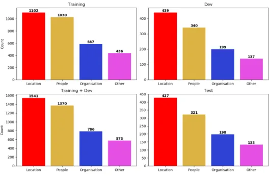
named entities. The distribution of each type of named entity can be found in Figure 6.

The distribution of the named entity types is roughly the same across all different datasets. Location (1968) is the named entity type with the most

(31)

Figure 7: Relation types

appearances in the dataset with People (1691) following close behind while Organisation (984) and Other (706) occur about half as often.

All sentences contain at least one relation and two named entities are needed for a relation. Due to the distribution of the named entity types, certain relations occur much more frequently than others. The distribution of the relation types can be found in Figure 7. Unlike the distribution of the named entity types, the distribution of the relation types is not very similar across the different datasets. Live In (521) is overall the relation type with the most appearances. OrgBased In (452) is the second most common relation type. Located In (406) and Work For(401) are approximately equally represented in the dataset while Kill (258) has a noticeably low amount of occurrences. The distribution of relation types in each set however does not follow the same principle. The relation Live In for example has the highest amount of appearances in the training and the dev set while having the second highest

(32)

amount of occurrences in the actual test set. Located In has a low number of occurrences in the training set while being close to the top in both dev and test. The relation Kill at least has the lowest amount of appearances across sets. The different distribution of the validation set might stem from its creation by random sampling.

(33)

5 Models

In this section the models used for named entity classification and relation classification for each level are defined. Entities and relations are extracted from a sentence. As described in Section 4 entities can span over multiple tokens and relations are directed. For extracting relations by multinomial classification, a new relation called ”N” is created. This relation type signi-fies there is no relation between two probed entities. The investigation distin-guishes between four different levels of joining entity and relation classifica-tion. The data is usable after undergoing data preprocessing like described in Section 4. The predicted labels are compared with the expected labels at the end of each model returning a classification report, which includes precision, recall and F1 score.

5.1 Level One

In Level one a pipeline of independent models for entity and relation classi-fication is used. The model used for entity classiclassi-fication was first introduced by Lafferty et al. (2001). In the first step, a linear-chain CRF is used to recog-nize and classify entities by setting a sequence of tokens with corresponding features as the input and expecting a sequence of named entity types (labels) as output. A predicted label counts as correctly predicted if the entire label matches the entire named entity type with BILOU encoding. After predict-ing the entity labels, the predicted data is restructured to fit into the needed form to extract relations. In this process, all tokens with a predicted label that is not a named entity type are ignored. Thus, only tokens with a label of a named entity types will be left. All sequential entities with the same entity type are grouped into one entity with ”B-” and ”L-” being the start and the end of an entity boundary (likewise with ”U-”). Then all entities in a sentence are put against all other entities in the same sentence meaning there arey = (n−1)·n(∀n >1) many possibilities of relation pairs fornextracted

(34)

SentenceID Entity1 Entity2 Relation

10 Israel Tuvia Tzafir N

10 Tuvia Tzafir Israel Live In

Table 6: Showing relation pairs of two entities. All other columns in this DataFrame are omitted as they would only cluster the table; Multi-token entities are treated as a single entity and any relations are mapped on the respective last token of the multi-token entity

entity pairs. The order of the relation is reflected by the order of the entities in the table: Entity1 ⇒ Entity2. An example table demonstrating this can be found in Table 6. Similar to Miwa and Sasaki (2014) relations on entities are mapped on the last words of the entities. In the last step the entity pair (Entity1, Entity2) in a vectorized form and a FeatureVector as described in Section 5.6 are used as input for the respective classifier.

5.2 Level Two

Level two utilizes the same aforementioned model although the model now includes entity type predictions as input for the classifiers as described by Giuliano et al. (2007). The best results have been achieved using only the named entity type prediction excluding the BILOU label.

5.3 Level Three

Level three uses global features to make more accurate predictions on the test set. The level three models still use local features as the level two models and global features in addition. In particular, the predictions of the entity

(35)

clas-sification are used for relation clasclas-sification and afterwards the predictions of relation classification are used to predict better named entity tags. The predictions of linear support vector machines have been utilized as global features for entity-relation.

5.4 Level Four

Level four uses a model to join entity and relation classification. A linear-chain CRF is used to classify the data after being fitted on the train set. A sequence of tokens with corresponding features is the input and a sequence of the following format is the output:

• Y −ARGX +Z.

• X is the number of the argument. As relations are directed, the relation has a first and a second argument. X is the identifier of the relation argument.

• Y is a relation type such as Live In or Kill of the token (or phrase)

• Z is the BILOU label of the token (or phrase)

• Examples: ”Live In-ARG1+B” or ”Kill-ARG2+U”

If the token does not participate in any relations a simple ”N” will be given as the label. Table 7 shows already preprocessed data with the new label. As the input only expects a binary classification problem, the model has to be run multiple times with different relation types as labels with the same model type (CRF). Thus, one model is used for each relation type. The model cannot include entities with multi-labels (ARG1 and ARG2 for the same re-lation type). Therefore all tokens with multi-labels are modelled into tokens with one label. As this only happens in a miniscule amount of cases (around 1%) it should not affect the evaluation. Evaluating the predictions is not as

(36)

SentenceID Token NER Relation Label

10 Israel U-Loc Live In Live In-ARG2+U

10 television O N N 10 rejected O N N 10 a O N N 10 skit O N N 10 by O N N 10 comedian O N N

10 Tuvia B-Peop Live In Live In-ARG1+B

10 Tzafir L-Peop Live In Live In-ARG1+L

· · · ·

Table 7: Result of restructuring the data of sentence 10 to fit the model used for level 4. In comparison to Table 6, all tokens have to be relabeled.

simple as it was for level one to three. First the tokens have to be converted into entities respective to their predicted label. As the order is already estab-lished there is no reason to determine the direction as seen in Table 6. Thus, only the predicted order is saved. A relation counts as correctly predicted if the entity boundaries are accurate and the order of the entity pair and the order of the arguments is correct. For entity classification the model chooses the predicted BILOU label and concatenates it with the appropriate named entity tag related to the position of the entity in the argument (see Table 3). Thus, only entities that participate in relations can be recognized. The entity type ”Other” cannot be predicted using this model since this entity type does not participate in any relation.

Figures 8 and 9 showcase the different models. Figure 8 shows the model of level one to three while Figure 9 shows the model of level four. All tokens that do not participate in relations have the label N.

(37)

Figure 8: Model of level one to three of the sentence ”Apple Inc. is based in Cupertino, California”. The color red is used to mark features introduced by level two while the color green is used to mark features used for entity classification of level three.

Figure 9: Model of level four of the sentence ”Apple Inc. is based in Cupertino, California”. Two different relations are found in the sentence indicating the usage of two different CRF models.

(38)

5.5 Hyperparameters

Hyperparameter optimization has been performed on named entity classifi-cation of levels one to three and on the joint model of level four. The opti-mization has been performed on regulation parameters (c1, c2) of the CRF classifier using randomized search and 3-fold cross-validation. The model was fitted 50∗3 = 150 times during the process. Hyperparameter optimization on the joint model of level four was done in a similar way for all relation types.

Optimizing the classifiers for relation classification has been done on a much smaller scale as hyperparameter optimization of five different classifiers per level is computationally expensive. Thus, only the parameter class weight

has been optimized for all classifiers. The LinearSVC classifier underwent an additional optimization process of finding the best value ofCamong multiple values. Parameters can be found in the appendix in Table 24.

5.6 Features

In this section the features are explained. The features for words (entities) are similar to the features used by Florian et al. (2003) and Miwa and Sasaki (2014). Some features are more general and the gazetteer information is ex-cluded. For relations, a variety of different features is used. Cross-task fea-tures for entity recognition and classification are used in level three to repre-sent dependencies between entity and relation. (Shortest) Dependency paths features are similar to Xu et al. (2015). The features used for each level can be found in the Table 8 to 11. The features marked with colour indicate fea-tures that are introduced in that respective level. Feafea-tures marked with red are introduced in level two and features marked with green are introduced in level three. The colours are similar to the colours used in Figure 8.

(39)

Target Category Features

Entity Lexical Word (first 2/3 characters)

Word types (word lower, initial-capitalized, all-digits, all-puncts, title) Part-Of-Speech Tags ( + pos bigrams) Contextual Word (+ word bigrams within a

con-text window of 3 words (i-1,i,i+1) Word types (as described) in a context window of 3 words (i-1,i,i+1)

PoS-tags within a context window of 3 words(i-1,i,i+1)

Begin of Sentence, End of Sentence Relation Entities Entities in bag-of-words model

Contextual Sentences (bigrams of characters) in which the entities appear

Shortest path

Shortest dependency path between two entities (entity1-dependency-entity2) The length of the paths

(40)

Begin of Sentence, End of Sentence Relation Entities Entities in bag-of-words model

Shortest path

Entity type

Predictions of entity label for each en-tity

Table 9: Features for Level 2. The features which are different to level 1 are highlighted in red.

(41)

Begin of Sentence, End of Sentence

Entity-relation

Relation label and the label of its par-ticipating entity

Relation Entities Entities in bag-of-words model

Shortest path

Entity type

Predictions of entity label for each en-tity

Table 10: Features for Level 3. The features which are different to level 2 are highlighted in green.

(42)

Target Category Features Entity and

Relation

Lexical Word (first 2/3 characters)

Begin of Sentence, End of Sentence Adjacency

nodes

Adjacency nodes of all words from the dependency tree

(43)

5.7 Implementation Methods

Python has been chosen as the programming language to implement the models as Python offers various libraries dedicated to natural language pro-cessing and machine learning.

Scikit-learn3 _{offers simple and efficient tools for data mining and data}

ana-lysis built on NumPy, SciPy and matplotlib. Scikit-learn is an open source library offering a wide range of state-of-the-art machine learning algorithms for supervised and unsupervised learning (Pedregosa et al., 2011). Used al-gorithms and methods for this thesis include CountVectorizer, a converter of text documents into matrices of token counts and the implementations of classifiers such as linear support vector machines.

Pandas4 _{is an open source library providing data structures and data}

anal-ysis tools for Python. Pandas.DataFrames are the primary data structure of pandas. DataFrames are two-dimensional tabular data structures with la-beled axes, capable of allowing arithmetic operations on both row and column labels and mutable in size. In the context of this thesis, DataFrames are used to store all data in a flexible structure.

SpaCy5 _{is a free open source library for NLP in Python. Alongside its wide}

area of NLP related tasks, it offers labelled dependency parsing. As our fea-tures include the dependency grammar, a combination of SpaCy and Net-workX6 are used to create the graphs using trained tokenization models7. NetworkX algorithms are then applied to find the shortest path between two words in a graph and to calculate the length of the path. Furthermore, adjacent nodes within the graph are found and used as features for level four.

3_{http://scikit-learn.org/stable/} 4_{https://pandas.pydata.org/} 5_{https://spacy.io/}

6_{https://networkx.github.io/} 7_{https://spacy.io/usage/models}

(44)

6 Results and Analysis

In this section, the experiments and their results will be presented and ana-lyzed.

6.1 Experiments and Results

The models have been applied to the development set for validation and hy-perparameter tuning and the test set for testing. The results of entity recog-nition and classification can be found in Table 12 and 13. Table 14 shows the results of each entity type with BILOU encoding for each level while Table 12 shows the results of each level for entity classification. All entity types (including Other) are included in the table. The results of level four are excluded as it uses a different model and therefore only includes named entities that participate in relations. Thus, the results are not comparable. The results of named entity recognition and classification for level four can be found in the appendix (see Figure 25 and Figure 26). Level one and level two use the same model for entity classification and hence their results are identical. The results show that level three has the best overallF1 score with

a value of 0.830. Level one and level two are equal with anF1 score of 0.815.

There is no noticeable discrepancy between precision and recall for level one and two. A slight discrepancy exists for level three as the score for recall is about 0.1 worse than the score for precision. Level four has a comparable precision score with 0.822. The accuracy score is comparable across all levels with level three having slightly better results than level one and two.

Table 13 shows the results of each level for entity classification with the ex-clusion of the entity typeOther and an exclusion of the results of level four as aforementioned. The results for the remaining entity types Person, Location andOrganisation are displayed in the table above. Level three has the overall best results for Person and Organisation, with 0.884 and 0.816 respectively while having the second best result of Location with anF1score of 0.811. The

(45)

Level All Entities Accuracy Level 1 0.828 / 0.810 / 0.815 0.940 Level 2 0.828 / 0.810 / 0.815 0.940 Level 3 0.881 / 0.796 / 0.830 0.943

Table 12: Results of entity classification with all entity types (including Other) on the test set (precision / recall / F1 score)

Level 1 & 2 Level 3

Person 0.838 / 0.905 / 0.869 0.889 / 0.880 / 0.884 Location 0.880 / 0.806 / 0.838 0.914 / 0.744 / 0.811 Organisation 0.739 / 0.747 / 0.741 0.844 / 0.794 / 0.816 Average 0.819 / 0.819 / 0.816 0.884 / 0.806 / 0.837 Table 13: Results of entity classification with named entity types (excluding Other) on the test set (precision / recall / F1 score)

model of level one and two offers slightly worse results. The precision scores of level four are nearly ideal for entity types Person and Location with 0.947 and 0.991 respectively. Table 14 is validating this observation. The entity type Location has the best precision scores with Person having the overall best recall scores and hence the best overall F1 score. The labelU-Other has

(46)

Level 1 Level 2 Level 3 Level 4 B-Loc 0.91/0.76/0.83 0.91/0.76/0.83 0.98/0.66/0.79 1.00/0.37/0.54 I-Loc 0.95/0.69/0.80 0.95/0.69/0.80 0.97/0.58/0.73 1.00/0.52/0.68 L-Loc 0.88/0.74/0.80 0.88/0.74/0.80 0.98/0.66/0.79 1.00/0.37/0.54 U-Loc 0.85/0.89/0.87 0.85/0.89/0.87 0.83/0.87/0.85 0.98/0.34/0.51 B-Org 0.69/0.72/0.70 0.69/0.72/0.70 0.81/0.80/0.81 0.85/0.38/0.53 I-Org 0.69/0.77/0.73 0.69/0.77/0.73 0.89/0.87/0.88 0.76/0.38/0.50 L-Org 0.76/0.80/0.78 0.76/0.80/0.78 0.83/0.82/0.82 0.92/0.40/0.56 U-Org 0.86/0.67/0.76 0.86/0.67/0.76 0.85/0.62/0.72 1.00/0.28/0.43 B-Peop 0.82/0.88/0.84 0.82/0.88/0.84 0.89/0.89/0.89 0.92/0.55/0.69 I-Peop 0.82/0.95/0.88 0.82/0.95/0.88 0.94/0.91/0.92 0.98/0.68/0.80 L-Peop 0.87/0.94/0.91 0.87/0.94/0.91 0.89/0.89/0.89 0.94/0.56/0.70 U-Peop 0.83/0.81/0.82 0.83/0.81/0.82 0.80/0.78/0.79 1.00/0.29/0.45 B-Other 0.89/0.74/0.81 0.89/0.74/0.81 0.94/0.79/0.86 * I-Other 0.84/0.70/0.76 0.84/0.70/0.76 0.91/0.76/0.83 * L-Other 0.87/0.73/0.79 0.87/0.73/0.79 0.91/0.76/0.83 * U-Other 0.58/0.45/0.51 0.58/0.45/0.51 0.54/0.39/0.45 *

Table 14: Results of entity classification visualized with all entity types in BILOU encoding (precision/recall/F1 score). The * selected cells cannot be

(47)

Table 15 shows the results of each classifier used for relation extraction and classification for all levels. Five different classifiers have been used to extract and classify relations: Linear Support Vector Machine (LinearSVC), Decision Tree Classifier (DTC), Perceptron, Stochastic Gradient Descent Classifier (SGDC) and Maximum Entropy (MaxEnt). The arithmetic mean is added below the results for each level. Due to the different model of level four the relation extraction and classification of level four is done via linear-chain CRF with and without graph features. The used features can be found in Section 5.6.

The results for level one are mixed. DTC and SGDC have low F1 scores

with 0.32 and 0.36 respectively, whereas LinearSVC, Perceptron and Max-Ent have about 20% higher F1 scores with around 0.44. The accuracy score

is about equal for all classifiers with a value of approximately 0.89. There is, however a noticeable discrepancy between precision and recall for LinearSVC and DTC. Consequently, LinearSVC performs the best for level one and DTC performs the worst.

Level two sees distinguished improvements on all sides compared to level one. All classifiers have increased recall and F1 scores with LinearSVC and

Perceptron being the best classifiers with an F1 score of 0.54. While

preci-sion went down for LinearSVC and SGDC, the increase of recall raised the

F1 score. Particularly the enhancement of the decision tree classifier is

no-ticeable. With an increase of its recall score from 0.24 to 0.43, which is nearly an increase of 100% it augmented its F1 score from a poor 0.32 to a solid

0.49. There are no huge differences when comparing the results of level two to the results of level three. SGD Classifier saw a small increase of 0.04 while the other classifiers stayed mostly the same. Thus, level three offers slightly better results than level two and given the results of the other levels, the best results of all levels with an average F1 score of 0.52.

(48)

Level 1

Classifier All Relations Accuracy LinearSVC 0.66 / 0.36 / 0.46 0.912 DTC 0.51 / 0.24 / 0.32 0.897 Perceptron 0.52 / 0.41 / 0.44 0.881 SGDC 0.45 / 0.36 / 0.36 0.876 MaxEnt 0.50 / 0.42 / 0.44 0.888 avg/total 0.53 / 0.36 / 0.40 0.891 Level 2 LinearSVC 0.62 / 0.49 / 0.54 0.914 DTC 0.60 / 0.43 / 0.49 0.914 Perceptron 0.55 / 0.55 / 0.54 0.897 SGDC 0.40 / 0.59 / 0.46 0.857 MaxEnt 0.50 / 0.56 / 0.52 0.892 avg/total 0.53 / 0.52 / 0.51 0.895 Level 3 LinearSVC 0.58 / 0.49 / 0.53 0.915 DTC 0.61 / 0.44 / 0.49 0.914 Perceptron 0.53 / 0.55 / 0.53 0.894 SGDC 0.47 / 0.55 / 0.50 0.878 MaxEnt 0.49 / 0.58 / 0.53 0.892 avg/total 0.54 / 0.52 / 0.52 0.899 Level 4 CRF Graph 0.82 / 0.28 / 0.42 0.913 CRF 0.86 / 0.31 / 0.43 0.915 avg/total 0.84 / 0.30 / 0.42 0.914

Table 15: Results of relation extraction on the test set and using (precision / recall / F1 score) and accuracy to evaluate

(49)

The results for level four show two linear-chain CRFs. One used graph fea-tures such as adjacency nodes while the other did not include graph feafea-tures. Comparing the two models returns almost identical F1 scores of 0.42 for a

CRF with graph features and 0.43 for a CRF without graph features. The recall scores follow the same scheme, whereas the precision scores show slight differences with the CRF without graph features being marginally better than the CRF with graph features. Level four has slightly better accuracy scores compared to the other levels. However, accuracy as an evaluation metric is flawed when it comes to an unbalanced amount of positives and negatives. Thus, predicting N for all cases always results in high accuracy scores. Con-sequently, the F1 score is the better alternative to compare results.

Table 16 and 17 show the results of each relation type for each classifier and level. Table 16 includes the relation typesKill,Live In andLocated In whilst Table 17 shows the results of relation typesWork For andOrgBased In. The first noticeable thing about the table is the fact that the relation type Kill has by far the best F1 score of all relations with the DTC reaching 0.90 for

level two and three. By way of contrast, the relation Located In has by far the worstF1 score reaching a value of 0.38 at best while using the perceptron

classifier for level two and three. The results of OrgBased In and Work For are more or less equal while the results for Live In are worse.

Moreover, Table 27 in the appendix shows the results of the used model for level four. Here, the F1 scores for each argument of each relation are

dis-played. Additionally, each argument was split into all possible BILOU labels to provide further information. CRF Dev describes the result on the valida-tion set while CRF Test and CRF Test Graph describe the results on the test set without graph features and with graph features. In short, the precision scores are very high while the recall scores are somewhere between very low and very good, as seen in all labels starting with Kill. Thus, performance of the model is not as stable as the performance of level two and three.

(50)

Level 1

Kill Live In Located In

LinearSVC 0.84/0.79/0.81 0.64/0.27/0.38 0.43/0.21/0.29 DTC 0.88/0.64/0.74 0.48/0.22/0.30 0.35/0.09/0.14 Perceptron 0.68/0.81/0.74 0.44/0.31/0.36 0.22/0.38/0.28 SGDC 0.45/0.89/0.60 0.46/0.19/0.27 0.30/0.17/0.22 MaxEnt 0.68/0.85/0.75 0.46/0.28/0.35 0.32/0.32/0.32 Level 2 LinearSVC 0.79/0.79/0.79 0.50/0.55/0.53 0.49/0.21/0.30 DTC 0.93/0.87/0.90 0.54/0.43/0.48 0.40/0.11/0.17 Perceptron 0.75/0.83/0.79 0.39/0.58/0.47 0.35/0.41/0.38 SGDC 0.66/0.89/0.72 0.39/0.58/0.47 0.42/0.26/0.32 MaxEnt 0.66/0.87/0.75 0.40/0.59/0.48 0.34/0.38/0.36 Level 3 LinearSVC 0.79/0.79/0.79 0.49/0.51/0.50 0.45/0.24/0.32 DTC 0.93/0.85/0.89 0.52/0.38/0.44 0.52/0.14/0.22 Perceptron 0.76/0.81/0.78 0.39/0.53/0.45 0.32/0.45/0.38 SGDC 0.51/0.91/0.65 0.43/0.54/0.48 0.27/0.44/0.33 MaxEnt 0.67/0.85/0.75 0.41/0.55/0.47 0.34/0.41/0.37 Level 4 CRF Graph 0.89/0.72/0.80 0.92/0.23/0.37 0.62/0.20/0.30 CRF 0.87/0.72/0.79 0.95/0.19/0.32 0.72/0.20/0.30 Table 16: Results of relation extraction (i) on the data set using (precision / recall / F1 score) to evaluate

(51)

Level 1

OrgBased In Work For LinearSVC 0.82/0.43/0.56 0.64/0.30/0.41 DTC 0.56/0.29/0.38 0.46/0.14/0.22 Perceptron 0.80/0.34/0.48 0.51/0.45/0.48 SGDC 0.69/0.34/0.46 0.30/0.49/0.37 MaxEnt 0.72/0.39/0.51 0.37/0.49/0.42 Level 2 LinearSVC 0.70/0.54/0.61 0.69/0.50/0.58 DTC 0.61/0.50/0.55 0.71/0.49/0.58 Perceptron 0.75/0.51/0.61 0.63/0.55/0.59 SGDC 0.29/0.70/0.41 0.44/0.67/0.53 MaxEnt 0.58/0.56/0.57 0.59/0.55/0.57 Level 3 LinearSVC 0.67/0.55/0.61 0.62/0.49/0.53 DTC 0.62/0.50/0.56 0.62/0.53/0.57 Perceptron 0.71/0.51/0.60 0.59/0.58/0.58 SGDC 0.62/0.46/0.53 0.52/0.63/0.57 MaxEnt 0.58/0.58/0.58 0.56/0.64/0.60 Level 4 CRF Graph 0.88/0.28/0.43 0.71/0.16/0.26 CRF 0.92/0.31/0.47 0.77/0.17/0.28

Table 17: Results of relation extraction (ii) on the data set using (precision / recall / F1 score) to evaluate

(52)

6.2 Analysis

The previous section introduced and presented the experiments the results. The goal of this section is a comprehensive analysis of the results for both, entity and relation classification starting from level one. The analysis of the results of entity and relation recognition and classification will be divided into two parts. First, the entity and relation classification for level one, two and level three will be analysed and evaluated and then the joint approach for level four will be examined.

Level 1 & 2 Level 3

Top Likely

I-Org ⇒ L-Org 7.5 B-Org ⇒L-Org 6.5 B-Org⇒L-Org 7.1 B-Org ⇒I-Org 6.4 B-Loc ⇒L-Loc 7.0 I-Org ⇒L-Org 6.2 B-Org⇒I-Org 6.6 I-Org ⇒I-Org 6.0 I-Org ⇒I-Org 6.6 B-Loc ⇒ L-Loc 6.0 B-Loc ⇒I-Loc 6.6 B-Peop ⇒ L-Peop 5.9 I-Peop⇒L-Peop 6.2 I-Peop ⇒ L-Peop 5.6

Bot Likely O⇒ I-Org -4.2 O ⇒ L-Loc -2.1 I-Other ⇒O -4.1 B-Loc ⇒ O -2.1 O⇒ L-Loc -3.6 O ⇒ I-Peop -2.0 O⇒ I-Other -3.3 O ⇒ I-Org -2.0 B-Other ⇒O -3.3 B-Org ⇒O -1.7 B-Loc ⇒ O -3.2 O ⇒ L-Peop -1.5 I-Loc ⇒O -3.1 B-Peop ⇒ O -1.5 Table 18: Transitions of CRF labels

(53)

6.2.1 Entity Classification

Table 14 is an extensive spreadsheet showcasing the results for all possible labels. The first step in analyzing the CRF layer is the extraction of the most (and the least) likely transitions and the extraction of indicating words. Table 18 shows the seven most and least likely transitions while Table 19 displays the five top positive and negative words for level one to three. All correlations and transitions between entity types are accurate. It is very likely that the beginning of an organisation name is followed by a token inside the name (I-Org) or a token at the end of the name of the organisation. The same applies for the relation type People. Transitions from and to tokens with the labelO are penalized. TheOrganisation labels have the most appearances in the table even though Organisation as an entity type has one of the worst F1

scores (see Table 13). However when looking at Table 19 there are no appear-ances of Org labels in the rows for level one and two. The first appearance of an Org label is on position 12 with ”+1:word.lower():nomination”. There is no appearance at all when looking at the top negatives. Thus even though Organisation as a label has the most likely transitions, it does not have many words indicating that the respective word does indeed belong to an Organ-isation. The tagging is however very good once the beginning token of a multi-token entity has been accurately labeled. Furthermore, the transition score may indicates a better performance for entity recognition and classifi-cation for level one and two than for level three but Table 19 weakens that particular sentiment as the top positives are dominated by all relation type features (global) with the prime example being ”relation:N” with an out-standing score of 12. The other relation types are all having positive scores indicating that the inclusion of relation types as features is very helpful for entity recognition. Another perk of including relation types as features is the usage of context as for example the label U-Peop has the negative feature ”-1:word.lower():in”. This means that the wordin before an entity implicitly denies the possibility of the entity being a person. Worth mentioning is the occurrence of an entity with two relation types which indicates a location.

(54)

Label Feature Score Level 1/2 Pos U-Other +1:word.lower():basque 7.12 U-Other word.lower():rice 6.6 O word[-2:]:94 5.2 U-Loc word.lower():beijing 5.0 U-Loc word.lower():france 4.6 Level 1/2 Neg O 1:word.lower():18th -4.0 O postag:NNP -3.7 O +1:word.lower():side -3.2 L-Peop +1:postag[:2]:NN -2.6 O +1:word.lower():plant -2.6 Level 3 Pos O relation:N 12.0

U-Loc relation: Located In 4.3

U-Peop relation: Kill 4.1

U-Org relation: Work For 3.7

. . . .

U-Loc relation: Located In OrgBased In 3.2

Level 3 Neg

U-Other +1:postag[:2]:NN -2.5

L-Peop +1:postag:NNP -1.9

U-Peop -1:word.lower():in -1.8

Investigating different levels of joining entity and relation classification

Investigating Different Levels of

Joining Entity and Relation

Classification

Contents

1

Introduction

1.1

Goal of the Thesis

Structure of the Thesis

2

Related Work

3

Background

3.1

Evaluation Metrics

3.2

Part-of-Speech

3.3

Training, Test and Validation Sets

3.4

N-Gram

3.5

Vector Space Model and Bag-of-Words Model

3.6

Encoding with BILOU

3.7

Classification

3.8

Dependency Grammar

4

Data

4.1

Structure of the Data

4.2

Data Preprocessing

4.3

Data Statistics

5

Models

5.1

Level One

5.2

Level Two

5.3

Level Three

5.4

Level Four

5.5

Hyperparameters

5.6

Features

5.7

Implementation Methods

6

Results and Analysis

6.1

Experiments and Results

6.2

Analysis