Self-supervised Face Representation Learning

(1)

Self-supervised Face Representation

Learning

zur Erlangung des akademischen Grades eines

Doktors der Ingenieurwissenschaften

von der KIT-Fakultät für Informatik

des Karlsruher Instituts für Technologie (KIT)

genehmigte

Dissertation

von

Vivek Sharma

aus Siliguri, India

Tag der mündlichen Prüfung: 14. May 2020

Hauptreferent:

Prof. Dr.-Ing. Rainer Stiefelhagen

Karlsruher Institut für Technologie

Korreferent:

Prof. Dr.-Ing. Tamim Asfour

Karlsruher Institut für Technologie

(2)

(3)

Abstract

This thesis investigates fine-tuning deep face features in a self-supervised manner for discriminative face representation learning, wherein we develop methods to automatically generate pseudo-labels for training a neural network. Most importantly solving this problem helps us to advance the state-of-the-art in representation learning and can be beneficial to a variety of practical downstream tasks. Fortunately, there is a vast amount of videos on the internet that can be used by machines to learn an effective representation. We present methods that can learn a strong face representation from large-scale data be the form of images or video.

However, while learning a good representation using a deep learning algorithm requires a large-scale dataset with manually curated labels, we propose self-supervised approaches to generate pseudo-labels utilizing the temporal structure of the video data and similarity constraints to get supervision from the data itself.

We aim to learn a representation that exhibits small distances between samples from the same person, and large inter-person distances in feature space. Using metric learning one could achieve that as it is comprised of a pull-term, pulling data points from the same class closer, and a push-term, pushing data points from a different class further away. Metric learning for improving feature quality is useful but requires some form of external supervision to provide labels for the same or different pairs. In the case of face clustering in TV series, we may obtain this supervision from tracks and other cues. The tracking acts as a form of high precision clustering (grouping detections within a shot) and is used to automatically generate positive and negative pairs of face images. Inspired from that we propose two variants of discriminative approaches: Track-supervised Siamese network (TSiam) and Self-supervised Siamese network (SSiam). In TSiam, we utilize the tracking supervision to obtain the pair, additional we include negative training pairs for singleton tracks – tracks that are not

(4)

temporally co-occurring. As supervision from tracking may not always be available, to enable the use of metric learning without any supervision we propose an effective approach SSiam that can generate the required pairs automatically during training. In SSiam, we leverage dynamic generation of positive and negative pairs based on sorting distances (i.e. ranking) on a subset of frames and do not have to only rely on video/track based supervision.

Next, we present a method namely Clustering-based Contrastive Learning (CCL), a new clustering-based representation learning approach that utilizes automatically discovered partitions obtained from a clustering algorithm (FINCH) as weak super-vision along with inherent video constraints to learn discriminative face features. As annotating datasets is costly and difficult, using label-free and weak supervision ob-tained from a clustering algorithm as a proxy learning task is promising. Through our analysis, we show that creating positive and negative training pairs using clustering predictions help to improve the performance for video face clustering.

We then propose a method face grouping on graphs (FGG), a method for unsupervised fine-tuning of deep face feature representations. We utilize a graph structure with positive and negative edges over a set of face-tracks based on their temporal structure of the video data and similarity-based constraints. Using graph neural networks, the features communicate over the edges allowing each track’s feature to exchange information with its neighbors, and thus push each representation in a direction in feature space that groups all representations of the same person together and separates representations of a different person.

Having developed these methods to generate weak-labels for face representation learning, next we propose to learn compact yet effective representation for describing face tracks in videos into compact descriptors, that can complement previous methods towards learning a more powerful face representation. Specifically, we propose Temporal Compact Bilinear Pooling (TCBP) to encode the temporal segments in videos into a compact descriptor. TCBP possesses the ability to capture interactions between each element of the feature representation with one-another over a long-range temporal context. We integrated our previous methods TSiam, SSiam and CCL with TCBP and demonstrated that TCBP has excellent capabilities in learning a strong face representation. We further show TCBP has exceptional transfer abilities to applications such as multimodal video clip representation that jointly encodes images, audio, video and text, and video classification.

(5)

Abstract iii

All of these contributions are demonstrated on benchmark video clustering datasets:

The Big Bang Theory, Buffy the Vampire Slayer andHarry Potter 1. We provide extensive evaluations on these datasets achieving a significant boost in performance over the base features, and in comparison to the state-of-the-art results.

(6)

(7)

Acknowledgements

Firstly, I would like to thank my supervisor Rainer Stiefelhagen for his guidance, support, advice and most importantly, encouragement. I also thank Tamim Asfour for kindly agreeing to be a reviewer and helping to improve the quality of this thesis. I thank my main collaborators Ali Diba, M. Saquib Sarfraz and Makarand Tapaswi. They have been an inspiration to me. Their daily and sometimes weekly conversations have proved to be one of my best learning experiences during my Ph.D. thesis. Special thanks to Corinna Haas-Hecker for her help with the university’s administra-tive things and making me feel welcome.

I thank my previous supervisor, Luc Van Gool at KU Leuven/ETH Zürich. He is one of the most intelligent and inspiring people I have known. He taught me how to think outside of the box and introduced me to the field of computer vision.

I would also like to thank my other advisors at Massachusetts Institute of Technology, Harvard Medical School and Harvard University. Ramesh Raskar is to be thanked for his brilliant ideas and inspiration. Rajiv Gupta inspired me to work harder and better on problems that can impact billions of lives. Mauricio Santillana inspired me to work on tracking epidemic outbreaks. I thoroughly enjoyed our weekly conversations to bounce ideas off of and debate with.

I thank all other collaborators including Davy Neven, Michael S. Brown, Gabriela Csurka, Naila Murray, Diane Larlus, Ali Pazandeh, Hamed Pirsiavash, Veith Röth-lingshöfer, Mohsen Fayyaz, Manohar Paluri, Juergen Gall, Praneeth Vepakomma, Tristan Swedish, Ken Chang, Jayashree Kalpathy-Cramer, Congcong Wang, Faouzi Alaya Cheikh, Azeddine Beghdadi, Ole Jacob Elle, Jon Yngve Hardeberg, Sony

(8)

George, . . . for your support and help. The final three dots should be interpreted as the people I forgot to mention here and as an apology.

Further, during my Ph.D. thesis, I was lucky and fortunate enough to find wonderful numerous friends. Without their company my social life would have been incomplete. I would also like to thank them. These include Keni Bernardin (the most available, reliable and lively party guy I have known. Without you, I would have never known the real music: James Brown, funky jazz, acid jazz, blues and many more, thanks for that!), Ertunc Ertekin (my unstoppable boxing coach), André Nordbø (my always reliable soundboard for discussions), Haroon Mughal, Constantin Seibold (after 4am we start working), Sebastian Bullinger, Piyush Verma, Abhishek Singh, Subhash Chandra Sadhu, Himi Mathur, Connor Henley (Boston nightlife belongs to you!), Samuel Schöb (The Muddy Charles Pub misses you!), Kevin Marty (my MIT social backbone), Fatima Villa (coffee tastes better when you’re around), Guy Satat, Tjada Schult, Hao Li (the after MIT tech review party stays memorable!), Backtosch Mustafa (you indeed have impressive social skills - Harvard is complementary!), César Roberto de Souza, Uta Büchler, Patrick Buehler, Biagio Brattoli, Alessandra Bernardi, Rafael Rezende, Lagnojita Sinha, Tomohiro Maeda, Arun Nair (we share the pride of ACMMM’19 best paper together!), Eric Marengaux (you own Mont Aiguille!), Christoph Feichtenhofer, David Ross, Du Tran, Sourish Chaudhuri, Georg Buchner, Anca Nicoleta Ciubotaru, Pablo Galindo Zapata, Bert De Brabandere, Daniel Koester, Elsa Itambo, Amey Chaware, Ankit Ranjan, Syed Qasim Bukhari (the guy who knows the A-Z of human connections and communication), Ewa Szyszka, Prithvi Rajasekaran, Andres Mafla Delgado, Martin Humenberger (I agree, you told me, graduating earlier is better), Ferran Hueto Puig, Leonie Malzacher, Eva Schlindwein (my first awesome unofficial Ph.D. examiner - secret stays between us!),

. . .

Most importantly, I would like to thank my family for their inestimable support, understanding, love, care and believing in me.

(9)

List of Abbreviations

TSiam Track-supervised Siamese network . . . 5

SSiam Self-supervised Siamese network . . . 5

CCL Clustering-based Contrastive Learning . . . 6

FGG Face Grouping on Graphs . . . 6

TCBP Temporal Compact Bilinear Pooling . . . 6

MLP Multilayer Perceptron . . . 10

ReLU Rectifying Linear Unit . . . 10

CNN Convolutional Neural Network . . . 16

ELU Exponential Linear Unit . . . 16

SELU Scaled Exponential Linear Unit . . . 16

BBT The Big Bang Theory. . . .21

BF Buffy - The Vampire Slayer . . . 21

ACCIO Harry Potter 1 . . . 22

WCP Weighted Clustering Purity . . . 24

ACC Clustering Accuracy . . . 24

VAE Variational Autoencoder . . . 30

HAC Hierarchical Agglomerative Clustering . . . 35

BN Batch Normalization. . . .65

GCN Graph Convolutional Network . . . 78

FC Fully-Connected . . . 82

resGC residual Graph Convolution . . . 82

(14)

(15)

Basic Notations

Unless indicated otherwise, lower-case letters type-set in bold denote vectors, upper-case letters represent a matrix or tensor and lower-upper-case letters represent scalars.

(16)

(17)

List of Figures

2.1 Multilayer perceptron (MLP): an example neural network scheme with 3 layers. . . 10 2.2 Landscape of popular optimizers. Figure taken from Ruder(2016) . . 15 2.3 Common neural network architectures. . . 17 2.4 Common face recognition neural network architectures. . . 19 2.5 Example images for a few characters from our dataset. We show

one easy sample and one difficult sample. The extreme variation in illumination, pose, resolution, and attributes (spectacles) make the datasets challenging. . . 21 2.6 Co-occurrence matrix of ACCIO . . . 23 2.7 B3 _{metric explanation . . . 25}

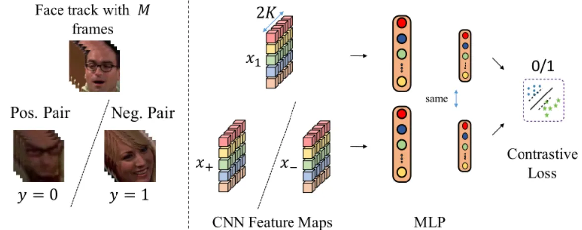
3.1 Track-supervised Siamese network (TSiam). Illustration of the Siamese architecture used in our track-supervised Siamese networks. Note that the MLP is shared across both feature maps. 2K corresponds to batch size. . . 34 3.2 Self-supervised Siamese network (SSiam). Illustration of the Siamese

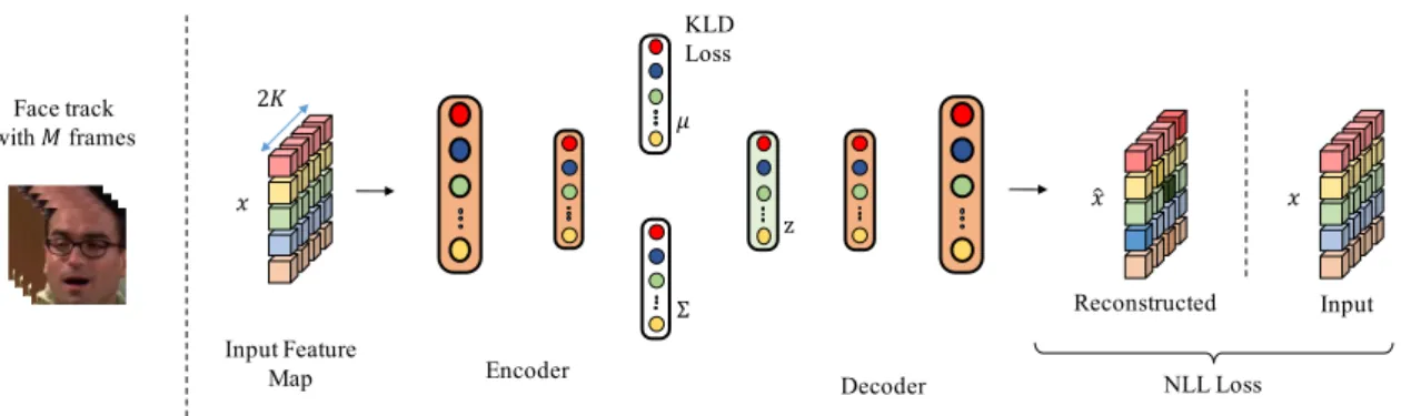
architecture used in our self-supervised Siamese networks. SSiam selects hard pairs: farthest positives and closest negatives using a ranked list based on Euclidean distance for learning similarity and dissimilarity respectively. Note that the MLP is the same across both feature maps. 2K corresponds to batch. . . 35 3.3 Illustration of a Variational Autoencoder used as a strong baseline

generative model. In contrast to the Siamese networks, the VAE sees single frames (not pairs) and is trained by two losses: KL-Divergence and the Reconstruction NLL. 2K corresponds to batch. . . 39

(18)

3.4 Illustration of the test time evaluation scheme. Given our pre-trained MLPs, TSiam or SSiam, we extract the frame-level features for the track, followed by mean pooling to obtain a track-level representation. All such track representations from the video are grouped using HAC to obtain a known number of clusters. . . 40 3.5 Histograms of pairwise cosine similarity between tracks of same identity

(positive, blue) and different identity (negative, red) for BBT-0101. Best seen in color. . . 43 3.6 Histograms of pairwise cosine similarity between tracks of same identity

(pos) and different identity (neg) for BBT-0101. . . 52 3.7 Histograms of pairwise cosine similarity between tracks of same identity

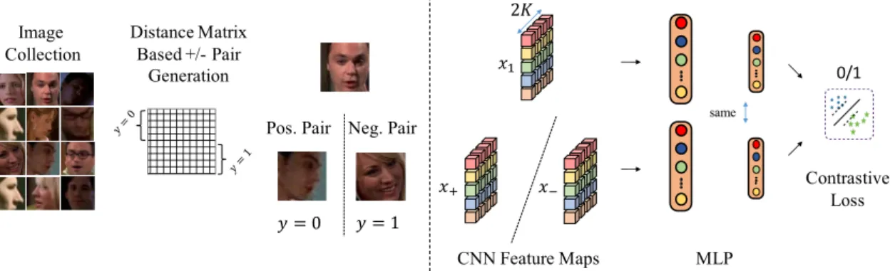
(pos) and different identity (neg) for BF-0502. . . 52 4.1 CCL training overview. Given a video with several face detections

(top left), we first start by extracting features using a deep CNN and perform clustering using FINCH to obtain a large number of small but highly pure clusters (top). We create several positive and negative face image pairs using these cluster labels and train an MLP to further improve the feature representation using the contrative loss (bottom). At test time, the MLP is used as an embedding, and we cluster our samples using Hierarchical Agglomerative Clustering (HAC). . . 60 4.2 Key characteristics of FINCH (second partition) clustering for

BBT-0101. Left: Histogram showing the number of faces in a cluster. Even if most clusters have less than 5 samples, we are able to obtain meaningful positive and negative pairs to train our model. Right: We plot the number of faces and number of tracks for each of the cluster indices (sorted by size for convenience). About 900 of the 2200 clusters created by FINCH contain faces from more than one track, leading to increased diversity of pairs. . . 69 5.1 Exemplary split of a toy graph: On the left a graph G = (S(T,1), Etc)

representing four temporally overlapping tracks. Each node represents a full track t ∈ T. No must-link edges are present. On the right G0 = (S(T,[1 3 1 1]), Etc∪Ecopy∪Etm), with trackt1 split into 3 sub-tracks.

The created nodes are t4, t5 and t6. All created nodes are completely

(19)

xvii

5.2 Our FGG model. The input is a matrix of all pooled sub-track features, the output is the updated representation of each sub-track. Note that the model never actually sees any images, they are just used to represent a sub-track here. The fully-connected layer uses the same weights for each track, i.e. the batch dimension is equivalent to|V|. . . 83 5.3 Training on BBT-0101 and BF-0502 with increasing edge dropout (left) and

added wrong edges (right). Each data point corresponds to one training run for 30 epochs. . . 91 5.4 Comparison of a PCA projection (Abdi and Williams, 2010) of feature

space at the start and end of training on BF-0502 and BBT-0101 using FGG. The ground truth character associations to each data point are color-coded. . . 95 5.5 Comparison of a t-SNE projections (van der Maaten and Hinton,2008) of

feature space at the start and end of training on BF-0502 and BBT-0101 using FGG. The ground truth character associations to each data point are color-coded. . . 96

6.1 Video ordering: Given an unordered collection of video clips, our goal is to infer their correct temporal order by utilizing a compact multimodal feature encoding that exploits high-level semantic concepts such as objects, scenes, dialogues, and sounds in each clip. We visualize five clips (first and last frame) from a scene in our dataset. Can you guess the correct order by considering all modalities? . . . 98 6.2 Deep Multimodal Feature Encoding. Illustration of the multimodal

feature encoding applied for the task of temporal ordering. See Sec. 6.3 for a detailed explanation of the feature learning scheme shown. . . . 103 6.3 CBP-Flat vs. TCBP. In this toy setup, we initialize random vectors

h, sand matrix S such thatc= 5,d= 7, and t= 3. In CBP-Flat,h

has different values across the temporal dimension, while in TCBP,

h does not depend on t. This ensures that Tensor Sketch projects features across time to the same output index. See Sec. 6.3.1 for a detailed explanation. . . 106 6.4 Examples scenes from the dataset with 2-4 clips. . . 113

(20)

(21)

List of Tables

2.1 Statistics of The Datasets. . . 22 3.1 Clustering accuracy on the base face representations. . . 42 3.2 Ignoring singleton tracks (and possibly characters) leads to significant

performance drop. Accuracy on track-level clustering. . . 43 3.3 Comparison between SSiam and pseudo-RF. . . 44 3.4 Clustering accuracy computed at track-level on the training episodes,

with a comparison to all evaluated models. . . 44 3.5 Clustering accuracy computed at track-level across episodes within

the same TV series. Numbers are averaged across 5 test episodes. . . 45 3.6 Clustering accuracy when evaluating across video series. Each row

indicates that the model was trained on one episode of BBT / BF, but evaluated on all 6 episodes of the two series. . . 46 3.7 Clustering accuracy when extending to all named characters within

the episode. BBT-0101 has 5 main and 6 named characters. BF-0502 has 6 main and 12 named characters. . . 46 3.8 In a similar spirit to Tapaswi et al. (2014b), we evaluate the number

of clusters we can reach when maintaining clustering accuracy/purity at 1. Lower is better. . . 47 3.9 Impact of training on combined dataset of BBT-0101, BF-0502, and NH. 47 3.10 Comparison to state-of-the-art. Metric is clustering accuracy (%)

evaluated at frame-level. Please note that many previous works use fewer tracks (# of frames) (also indicated in Table 2.1) making the task relatively easier. We use an updated version of face tracks provided byBäuml et al. (2013). . . 49

(22)

3.11 Performance comparison of TSiam and SSiam with JFAC (Zhang et al., 2016b) on ACCIO with 36 clusters. . . 50 3.12 Performance comparison of different methods on ACCIO with 40

clusters. . . 50 3.13 Clustering accuracy (%) performance comparison of TSiam, SSiam,

and VAE over all three dataset BBT-0101, BF-0502 and ACCIO . . . 51 4.1 Clustering accuracy of CCL and comparison to PRF (Yan et al.,2003b)

TSiam (Sharma et al., 2019a) and SSiam (Sharma et al., 2019a) at track-level. Comparison against all evaluated models. . . 66 4.2 Clustering accuracy of CCL and comparison to TSiam (Sharma et al.,

2019a) and SSiam (Sharma et al.,2019a) at track-level, extending to all named characters. BBT-0101 has 5 main and 6 named characters; BF-0502 has 6 main and 12 named characters. . . 66 4.3 A study on the impact of clustering algorithm. FINCH partitions

are created for each dataset, and shown as separate table rows. In each row, results are presented for FINCH (above) and MiniBatch

K-means (below). From left to right, Part. indicates the partition level of FINCH. #C is the total number of clusters in that partition as estimated by FINCH. Largest and smallest cluster sizes are indicated as LC/SC. Clustering purity of FINCH/K-means clusters (before CCL) is presented as ACC. L+/L- represents the number of samples correctly and wrongly clustered for the given partition. Finally, CCL-ACC is the performance of CCL: by training a model using weak labels from FINCH/K-means estimated clusters. . . 67 4.4 Impact of mining positive and negative pairs from different sources.

Track-level accuracy of CCL. . . 68 4.5 Comparison to state-of-the-art with clustering accuracy (%) at frame

level on both videos: BBT-0101 and BF-0502. . . 70 4.6 Frame-level clustering accuracy (%) of CCL and comparison to TSiam (Sharma

et al.,2019a) and SSiam (Sharma et al.,2019a) over all datasets: BBT-0101, BF-0502 and ACCIO. . . 70 4.7 Comparison of CCL with the state-of-the-art on ACCIO, evaluated at

(23)

List of Tables xxi

5.1 The layer structure for a graph G = (V, E). Note that |V| is dynamic and changes depending on the input episode. With several design choices, we optimized efficiently this network architecture that generalized over all datasets. . . 84

5.2 Comparison of WCP on each episode. The first row shows results when clustering the VGG2 (Cao et al., 2018) face representations of the main characters as they are contained in each dataset. The second row shows the performance of our proposed FGG model, averaged over 5 runs. Note that the standard deviation (std) is in units of permille (%). The drop in performance for BBT-0106 is caused by the nature of that episode: The characters are at a Halloween party wearing costumes. . . 86

5.3 WCP when evaluating across different episodes of the same dataset and a different dataset. We show values including and excluding the episode seen during training. Furthermore, we differentiate between evaluating each episode separately and then taking the mean (column separate), and clustering all features jointly (columnjoint). The best intra- and inter-series generalization is marked in bold. . . 88

5.4 Performance when evaluation on more and fewer characters than FGG is trained on. A comparison the previous works is presented in Table 5.5. . 89

5.5 Generalization to additional characters. We use the best model trained on the main cast as reported in Table 5.7. TSiam/SSiam and CCL are described in Chapter 3 (Sharma et al., 2019a) and Chapter 4 (Sharma et al.,2020) respectively. . . 89 5.6 WCP when training the FGG model with different features dis/enabled.

Mean and standard deviation are computed across 5 runs. See Sec-tion 5.4.2 for an explanaSec-tion of each experiment variaSec-tion. † indicates OUT_OF_MEMORY. . . 91

5.7 Comparison to state-of-the-art with clustering accuracy (%) at frame-level on both videos: BBT-0101 and BF-0502. Our result is the mean over five runs. . . 92

(24)

5.8 Influence of similarity-based edges on the ACCIO dataset. FGG-0 does not add any-similarity based edges. FGG-100* samples 100% of isolated nodes before splitting. This results in OUT_OF_MEMORY, indicated by †. FGG-100 computes similarity-based edges after splitting, and samples 100% of the remaining isolated nodes. Performance degrades slightly because connecting 3% of the nodes results in relatively more wrong edges compared to BBT and BF. . . 92 5.9 Performance comparison on ACCIO with 36 clusters. Score is averaged

over 5 runs. We achieve an absolute improvement of 18.5% in B3 F-Score over the previous state-of-the-art unsupervised learning method. . . 93 5.10 Performance comparison on ACCIO with 40 clusters. Score is averaged

over 5 runs. Our method outperforms previous unsupervised methods significantly, with 19% absolute improvement in B3 F-Score. . . 94 5.11 Frame-level clustering accuracy (%) of FGG and comparison to CCL (Sharma

et al., 2020), TSiam (Sharma et al., 2019a) and SSiam (Sharma et al., 2019a) over all datasets: BBT-0101, BF-0502 and ACCIO. . . 94

6.1 TCBP encodes several temporal segments without much additional overhead. Parameters c, t, d denote the number of channels, temporal segments, and the projected dimension. . . 107 6.2 Number of scenes in our dataset with 2-6 clips. . . 111 6.3 Temporal ordering performance with different t= 3 segment sampling

strategies and various modality combinations: A: Audio, P: Places, I: Objects, R: Video, and S: Subtitles/Text. . . 112 6.4 Ordering accuracy for varying number of clips per scene in the

valida-tion split. . . 114 6.5 Validation split ordering accuracy by changing the number of temporal

segments used to represent video clips. . . 114 6.6 Ordering performance with CBP and TCBP. More temporal segments

increases the gap between the two methods. . . 115 6.7 Comparing TCBP with other popular encoding strategies. . . 115 6.8 Role of negative mining for temporal ordering. . . 116 6.9 Multimodal retrieval results. The query set consists of 2770 clips, and

the test consists of 4466 clips, from 2443 scenes. TCBP with negatives.116 6.10 Qualitative top-3 retrieval results for a given query. . . 117

(25)

List of Tables xxiii

6.11 C3D ConvNets. Comparison of accuracy (%) of TCBP with C3D Con-vNet against state-of-the-art methods over all three splits of UCF101 and HMDB51. . . 118 6.12 Clustering accuracy computed at track-level on the training episodes,

with a comparison to all evaluated models. † indicates OUT_OF_MEMORY.120 6.13 Performance comparison of different methods when integrated with

TCBP on ACCIO with 36 clusters. † indicates OUT_OF_MEMORY.121 6.14 Performance comparison of different methods when integrated with

(26)

(27)

Chapter 1

Introduction

1.1 Objective and motivation

In this thesis we propose several methods to fine-tune deep face features in a self-supervised manner. Specifically, we address the problem of discriminative face representation learning in TV series and movies for face recognition tasks. Face representation learning has attracted quite some attention, due to the potential applications in video understanding, video summarization, content-based indexing & retrieval, video descriptions for visually impaired people, and more. We believe the performance of discriminative learning is driven by two factors: the (base) feature representation and the learning algorithm. It has been shown, a good initialized feature representation is complementary to the learning algorithm. An ideal representation has small distances between samples from the same class, and large inter-class distances in feature space. While considerable progress has been made using the current state-of-the-art learning algorithm - deep neural networks, learning a good representation often requires a large-scale dataset with manually curated ground-truth labels. On top of the challenges that make face recognition hard, there are issues like facial expressions, pose variations, ageing, occlusion and more. To harness the power of deep networks on smaller datasets and tasks, pre-trained models (e.g. VGG-Face (Cao et al., 2018; Parkhi et al., 2015) trained on a large number of face images) are often used as a feature extractors or fine-tuned for the new task.

(28)

Deep neural networks to learn powerful features for face recognition can be categorized into two paradigms: a fully-supervised setting where ground-truth labels are often provided by humans (Cao et al., 2018; Parkhi et al., 2015; Schroff et al., 2015; Taigman et al.,2014), and aself-supervised learning paradigm where no ground-truth labels are used for model training rather weak-information that come with the data for free are used for learning a representation. (Bäuml et al., 2013; Zhang et al., 2016a,b). This thesis falls in the pool of self-supervised learning setting where we generate weak-labels or pseudo-labels by learning objectives properly so as to get supervision from the data itself to learn discriminative face representations.

In the self-supervised learning paradigm for learning discriminative face representa-tions in videos, previously several attempts have been made. They mostly utilized pairwise constraints mined from face-tracks (Bäuml et al.,2013;Zhang et al.,2016a,b), such as themust-link constraint that two faces from the same track belong to the same person, and thecannot-link constraint that faces from tracks overlapping in time belong to different persons. These constraints are then used as a pairwise guide towards a suitable representation of each person in feature space using a loss function. Fortunately, there is a vast amounts of video material on television and the Internet that can be used by machines to learn an effective representation that exhibits a small intra-person-distance, and large inter-person-distance in feature space. This thesis develops self-supervised methods that can learn a strong face representation from large-scale data be in the form of images or video. Specific contributions are described Section 1.3.

1.2 Key challenges and tasks

There are many key challenges and tasks in dealing with the application of face recognition, here we list a few.

1.2.1 Key challenges

Appearance variations. In video face clustering, grouping all faces of the same person into a unique cluster is challenging, due to of several reasons, such as (a) variations in facial expressionse.g. anger, disgust, fear, happiness, sadness or surprise;

(29)

1.2.2 _{Key Tasks} 3

(b) pose variations around egocentric rotation angles i.e. pitch, roll and yaw, or camera changing point of views’ (c) variations in image resolution; (d) Presence or absence of structural components such as moustache, cap, and spectacles; (e) Partial face occlusion by foreground and background objects; (f) Ageing of the human face; and (g) Variations of illuminations, where low levels of lighting makes face detection and recognition hard, and high levels of lighting makes face overexposed. All the variations make the face clustering challenging.

Training data. For learning a good representation, training deep neural networks often requires a large-scale dataset with manually curated ground-truth labels. An-notation of video is expensive. For the approach to scale in the age of Netflix, YouTube and Instagram, where hundreds of hours of video material are uploaded to the internet per minute, it is vital that no manual annotation is required. The approach should furthermore not expect the ground-truth labels and rather utilize weak-information that come with the data for free for learning a good representation. In this direction, self-supervised learning has shown to be promising and usable in a general setting as collecting large-scale datasets is extremely expensive.

Speed and scalability. Nowadays, we have digital archives with huge collection of datasets, searching and indexing to find a certain specific person, object, or place is a common application. While retrieving specific instances through the video archival of hours of data and millions of frames, we expect the results to be real-time. Also, feature description is of paramount importance and needs careful design for representing faces in billions of images, such that they have: (a) Low computational overhead; (b) Extremely fast to compute; and (c) Scale to very large data and provide discrimination.

1.2.2 Key Tasks

Actor identification.An interesting multimedia application is actor identification, where the goal is to identify on-screen characters. While watching a movie or TV series, not always we remember all characters names in movie video. The objective is to identify on-screen character faces and label them with the corresponding names in the cast list. Usually, this automatic naming assignment is employed without any manual supervision and rather making use of textual cues, like cast lists, transcripts,

(30)

subtitles and closed captions. Netflix already provide these features and services to their customers.

Instances of person search. An important need in many conditions regarding video collections (archive video search/reuse, personal video organization/search, surveillance, law enforcement, protection of brand/logo use) is to locate more video segments of a certain precise person, object, or place, given a visual example. This is particularly useful on retrieving specific instances of persons in specific locations given a query image. This can save hours of efforts to manually look through the video archival.

Digital photo management.With the explosively increasing amount of personal photos, due to the rapid popularization of digital cameras and smart phones - there is a huge demand of digital photo management system for organizing photo collection. Recently several companies like Facebook, Google, Apple provide API services that provides a face-based album clustering and person search. The functionality of these API is to accurately and efficiently cluster photograph collections based totally on person identities, and group all faces of the same person into a small number of clusters.

Another rather unexpected application of digital photo management is in portrait collections, where the goal is to enable searching for portraits of famous identities. Portrait collection is of great importance to our cultural heritage as the collec-tion of portraits tell extraordinary stories of encounter, exploracollec-tion, independence, individuality and achievement of the famous identity.

1.3 Overview and Contributions

This thesis focuses on self-supervised face representation learning, wherein we pro-pose methods to automatically generate weak-labels for training a neural network. Specifically, we propose several self-supervised approaches to generate positive and negative face pairs utilizing the temporal structure of the video and similarity-based constraints to learn discriminative face representations. In this section, we list the main contributions made in this thesis. First in Chapter2, we give a brief introduc-tion of neural networks training. Following in Chapter 3 we propose a method to mine pseudo-labels by sorting distances on a subset of face images. In Chapter 4, we

(31)

1.3 _{Overview and Contributions} 5

propose a way to generate weak labels from a clustering algorithm and show how they can be used efficiently to improve video face clustering. In Chapter5we look at graph neural networks for self-supervised face grouping on graphs, wherein we utilize the video constraints: must-link/cannot-link constraints to generate weak-labels for model training. Finally in Chapter 6 we propose Temporal Compact Bilinear Pooling (TCBP) to encode face tracks in videos into a single descriptor, which we then integrate with methods presented in Chapter 3 and Chapter 4for learning a more powerful representation. The research covered in this thesis has resulted in several peer-reviewed publications. The contributions of each of these chapters are briefly discussed next.

Chapter 2briefly overviews background on the neural networks from basics building blocks to hyper-parameter optimization via training using back-propagation algorithm. We also discuss briefly the most popular convolutional neural networks for image classification and face recognition tasks. The aim of this chapter is to provide the reader an overview how a neural network is trained, and knowledge that is frequently needed in this thesis.

Chapter 3 proposes two discriminative approaches to refine the face descriptors au-tomatically: Track-supervised Siamese network (TSiam) and Self-supervised Siamese network (SSiam). In Track-supervised Siamese Network (TSiam), we utilize video-level constraints to generate a set of similar and dissimilar face pairs, and we further additionally include negative training pairs for singleton (non co-occurring) tracks by exploiting track-level distances. In Self-supervised Siamese Network (SSiam), we obtain hard positive and negative pairs by sorting distances on a subset of frames and not requiring video/track level constraints.

The content of this chapter is based on the following three publications:

• Vivek Sharma, M Saquib Sarfraz, and Rainer Stiefelhagen. “A simple and effective technique for face clustering in tv series”. In IEEE Computer Vision and Pattern Recognition (CVPR): Workshop on Brave New Motion Representations, 2017.

• Vivek Sharma, Makarand Tapaswi, M Saquib Sarfraz, and Rainer Stiefelhagen.

“Self-supervised learning of face representations for video face clus-tering”. In IEEE International Conference on Automatic Face and Gesture Recognition (FG), 2019. Oral presentation, Best paper award.

(32)

“Video face clustering with self-supervised representation learning”. IEEE Transactions on Biometrics, Behavior, and Identity Science (TBIOM), 2019.

In Chapter 4 we propose Clustering-based Contrastive Learning (CCL), a new clustering-based representation learning approach that uses labels obtained from clustering along with inherent video constraints to learn discriminative face features. Specifically, we show that we can train discriminative models using positive and negative pairs obtained through clustering and video-level constraints that do not rely on face tracking.

The content of this chapter is based on the following publication:

“Clustering based contrastive learning for improving face represen-tations”. In IEEE International Conference on Automatic Face and Gesture Recognition (FG), 2020.

In Chapter 5 we look at graph neural networks to learn face representations. We propose Face Grouping on Graphs (FGG), an approach to self-supervised face group-ing, where edges represent one of must-link/cannot-link constraints that emulates the communication. Using a neural network that operates on the graph structure and differentiates between the different edge types, the features can exchange information and assimilate their position in feature space compared to other features belonging to the same person. Additionally, we propose to work with partially pooled features as a trade-off between robustness on track-level and conservation of variance information on frame-level.

The content of this chapter is based on the following publication:

• Veith Röthlingshöfer*, Vivek Sharma*, and Rainer Stiefelhagen. “Self su-pervised face-grouping on graphs”. In ACM International Conference on Multimedia, 2019. Spotlight: oral presentation.

InChapter6 we propose Temporal Compact Bilinear Pooling (TCBP) an extension of the Tensor Sketch projection algorithm (Pham and Pagh, 2013) to incorporate a temporal dimension for representing face tracks in videos. We show that encoding

(33)

1.3 _{Overview and Contributions} 7

face tracks into a single descriptor are powerful in representing faces in images and videos.

The overall theme of this chapter is to learn multimodal clip representation that jointly encodes images, audio, video, and text using TCBP for video ordering task. Additionally, we show that TCBP features show exceptional transfer abilities to applications such as video classification, video retrieval and face video face clustering. The content of this chapter is based on the following publication:

• Vivek Sharma, Makarand Tapaswi, and Rainer Stiefelhagen. “Deep mul-timodal feature encoding for video ordering”. In IEEE International Conference on Computer Vision (ICCV): workshop on Large Scale Holistic Video Understanding, 2019. Oral presentation.

Finally, Chapter 7 concludes the thesis with a summary of the contributions, limitations and directions for future work.

(34)

(35)

Chapter 2

Background

In this chapter, we briefly overview the background information and theory related to the works presented in the manuscript. We first introduce to neural networks. We then explain the parameter estimators and learning: loss function, regularizer and training of neural networks. Finally, we present the popular neural network architectures, datasets and evaluation metrics used frequently in this thesis.

2.1 Neural Networks

Artificial neural network or neural network is the heart of the deep learning techniques. Neural networks are loosely inspired by neuroscience - biological neurons, and are designed to recognize patterns. The patterns they recognize are numerical, typically vector-valued. The neural networks can recognize patterns from the real-world data be it in the form of images, sound, text or time-series.

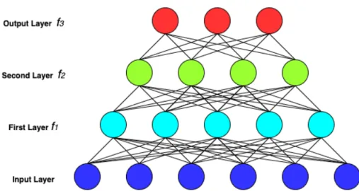
Given a training dataset with N samples D={xi,ci}Ni=1, where x∈Rm, andci is the vector of target labels corresponding to the input samplexi. A neural network is employed to learn a function f that maps an input xi to target-output ci. They are called networks because the learned function can be composed of multiple functions, connected in chain to forme.g. f(x) =f3(f2(f1(x))), wheref1 is the first layer of the

network,f2 is the second layer andf3 is the output layer of the network. ci represents the desired output of the f3 layer, while f1 and f2 are hidden layers and does not

represent the desired output. Each layer fk is parameterized by a learnable weight vector wk, fk(x) = φ(wkx), where φ is the activation function. The layer can be

(36)

Figure 2.1: Multilayer perceptron (MLP): an example neural network scheme with 3 layers.

viewed as a group of neurons, also called perceptrons where each neuron has inputs and learnable weights for each input that maps the vector input to a scalar output, also referred as Multilayer Perceptron (MLP). The activation function φ serves as a non-linearity, currently used most popular activation function being Rectifying Linear Unit (ReLU) (Glorot et al.,2011). They are used depending on the desired range of the neuron’s output, although other functions are also investigated. Neural networks can be seen as a universal approximator, meaning that if provided with enough neurons in the hidden layer and a suitable activation function. The learning of the neural network occurs through minimizing a loss function, i.e. the difference between the predicted output and the target output of the neural network. Because of the non-linearity of a neural network causes loss functions to become non-convex, neural networks are optimized by using iterative gradient descent steps on batches randomly sampled from the training set. The gradients of the loss function are computed using the back-propagation algorithm (Rumelhart et al.,1985) and the chain rule, meaning that we start from the last layers and backpropagate the estimated loss towards the preceding layers of the neural network. All the samples are shown during the training of the neural network in each epoch, and the process is repeated until convergence is reached. After a local minima is attained, the trained neural network is deployed for testing new samples that were not shown during the training phase. For a more extensive review on neural networks, we refer the reader toGoodfellow et al. (2016). Figure2.1 illustrates an example neural network scheme with 3 layers.

Often, matrix notations is used to describe the operations in a neural network. The weight of the layer fk is given as a weight matrix W ∈ Rn×m that transforms the

(37)

2.2 _{Learning: Parameter Estimators} 11

input x∈_Rn _to _y_∈

Rm following through the activation function φ. An additional

parameter, bias term (b) in the neural network is also added which is used to adjust the output along with the weighted sum of the inputs to the neuron, b∈_Rm_.

y=φ(Wx+b) (2.1)

During training a neural network, we aim to learn a set of weights for the neurons that minimizes the divergence between the predicted and target output using an appropriate loss function. The loss functions are task specific and are user defined.

2.2 Learning: Parameter Estimators

Although in this thesis, we focus on self-supervision only. Here, we explain learning for supervised setups aswell.

2.2.1 Loss Function

Regression loss. The aim of this loss is to predict a continuous value. Euclidean loss or L2-loss is the most commonly used regression loss function. L2 loss is the squared distance between the target output y and the network prediction ˆy. The L2 loss is given as:

L=kyˆ−yk2

2 (2.2)

L1 loss computes absolute differences between the target output and the network prediction. The loss is defined as:

L=kyˆ−yk1 (2.3)

Other popular regression loss functions e.g. Huber loss (Huber, 1992).

Classification loss. The aim of this loss function is to predict categorical value. The commonly used loss for classification is cross-entropy loss.

(38)

The softmax function is given as: Pq = exp(aq) PC r=1exp(ar) (2.4)

The cross entropy loss also known as softmax loss is defined as:

L=−

C X

q=1

yqlog(Pq) (2.5)

where a is the output of the last layer of neural network that is fed to a C-way softmax function, y is the vector of target labels for input data x, and C is the number of output classes.

Metric loss. The objective of this metric loss function is not to classify input samples, but to learn distances that exhibits small distances between samples for similar observations, and large distances for different ones. The commonly used metric loss functions are contrastive loss and triplet loss.

Contrastive loss. The contrastive loss (Hadsell et al., 2006) encourages small distances between samples from the same label, and far apart at least by the margin for the samples of different labels in feature space. The contrastive loss is given as follows: L= 1 2 (1−y)·(dW)2+y·(max(0, m−dW))2 (2.6) where dW is the euclidean distance between the sample pair x1,x2 with y= 0 for a

positive pair andy= 1 when corresponding to a negative pair, and m is the margin.

Triplet loss. The triplet loss (Schroff et al., 2015) encourages the distances between anchor and positive pair to be less than the distance between the anchor and negative by atleast distance margin. Triplet loss comprises of a pull-term, pulling data points from the same class closer, and a push-term, pushing data points from a different class further away. The triplet loss is formulated as:

L=max(d(x1,x2)−d(x1,x3) +m,0) (2.7)

whered is euclidean or cosine distance on the embedding space,mis the margin, and

x1, x2 and x3 are anchor, positive, negative respectively. x1, x2 andx3 are anchor,

(39)

2.2.2 _Regularizer 13

Other losses. There are several custom designed loss functions, specialized for different tasks, such as for geometric problems (Kendall and Cipolla, 2017), instance segmentation (Berman et al., 2018; Briggman et al.; De Brabandere et al.), dis-criminative face representation learning (Chopra et al., 2005; Schroff et al., 2015; Zhang et al.,2016a), image-caption retrieval (Vendrov et al., 2016) and many more tasks. In Chapter 3and Chapter 4, we propose loss functions for discriminative face representation learning and in Chapter 6 we propose to utilize a loss function for video representation learning.

2.2.2 Regularizer

A model that learns the train set too well and performs very poorly on the test set is a sign of overfitting. In such a case, the neural network has a very high variance and it cannot generalize well to the test data. Common ways to reduce overfitting are, (a) getting more training data; (b) use regularization to control the model variance. The commonly used regularization methods for neural networks are L2 regularization and dropout.

L2 regularization is also known as ridge regression or Tikhonov regularization. In L2 regularization, `2 norm penalty is added to the cost function that penalizes large

weights, and thus aim at limiting the model capacity.

Dropout randomly ignores nodes from a neural network during training to regularize it. The nodes are “dropped-out” randomly. That means other available neurons handle the representation required to make predictions. Thus, for each iteration, unique internal representations are learned by the network. In this way, the network becomes less sensitive to the specific weights of neurons, which in turn leads to better generalization and also helps to overcome from over-fitting.

(40)

2.2.3 Optimization

Once a neural network model, a loss function and a regularization is chosen, we can optimize the neural network to find the network parametersθ∗ that minimizes the cost function on the entire training set:

θ∗ = argmin θ

X

i

Li(fθ(xi),yi) (2.8)

The network parameters θ = (w,b), where (w,b) is the network weight and bias. The loss function computes loss for a single training example, while the cost function is average loss for the entire training set.

The most simple and naive way to optimize the neural network is to compute the derivative of the loss function wrt. the entire training set and then backpropagate the gradient through the preceding layers and update the network parameters. It is naive because of two reasons,

(a) It only relies on the first order information (i.e. the gradient). This can be addressed using different normalisation techniques.

(b) For computing the gradient it relies on the whole training set which is very expensive and practically not possible to compute for a large-scale dataset. This is usually addressed using a stochastic gradient descent (SGD) approximation.

Gradient Descent. The optimization is done using an iterative gradient descent optimization algorithm that makes use of the gradients to find local minima of the loss function i.e. iteratively moving in the direction of steepest descent. At each iteration, the gradients on each weight are computed using the back-propagation algorithm. Then, we update the parameters of the network, by taking a small step in the direction as defined by the negative of the gradient:

θ(t+1)=θ(t)−η ∂L

∂θ(t) (2.9)

whereη is the learning-rate and it determines the size of the step. ηshould be chosen carefully: if a very low learning rate is used, this may lead to slow convergence, and if a high learning rate is used, this may risk overshooting the lowest point and thus the training may not converge at all. SGD was used extensively in the thesis.

(41)

2.2.3 _Optimization 15

Figure 2.2: Landscape of popular optimizers. Figure taken fromRuder (2016)

Other popular optimizers are Adagrad, Adam, Adadelta, RMSProp (Duchi et al., 2011;Kingma and Ba, 2015; Qian, 1999;Zeiler, 2012). For a more detailed review on optimizer, we refer the reader to Ruder (2016). Figure2.2 shows the convergence behaviour of popular optimizers.

Back-Propagation. The back-propagation algorithm (Rumelhart et al.,1985) also known as backprop, allows to compute the gradients. Back-propagation is the method for computing the gradients of the loss function, while SGD is used to perform learning this gradient. Back-propagation adjusts each weight in the neural network in proportion to the loss function. Back-propagation is merely an application of the chain rule to find the derivatives of loss function with respect to the network parameters. The process of computing the gradients passing through preceding n

(42)

layers with activationsyi upto i-th layer for each weight wi from the loss function L is known as back-propagation, given as:

∂L ∂wi = ∂L ∂yn · ∂yn ∂yn−1 . . .∂yi−2 ∂yi−1 · ∂yi−1 ∂yi · ∂yi ∂wi (2.10)

In the next section, we discuss the convolutional neural networks, and the commonly used neural network architectures for image classification and face recognition.

2.2.4 Convolutional Neural Network (CNN)

Convolutional neural networks (LeCun et al., 1989) are simply an extension of multilayer perceptrons. Convolutional neural networks are also known as ConvNets. The basic difference between MLPs to ConvNets is that the linear layers are replaced by convolutional layers. ConvNets are easier to train and have shown to generalize better than feedforward networks or MLPs for vision tasks.

A Convolutional Neural Network (CNN) is composed of a stack of convolutional filter banks, each followed by the activation layer or non-linearity layer, and the pooling function or feature pooling layer. Each convolution layer takes an input feature map and outputs a new feature map through a set of weights called filter banks. In the convolution layer, the weights are shared that reduces the number of trainable parameters, and also since the feature map share the filter bank this benefits the convolution layers to be translation equivariant, meaning if the input changes, the output changes in the same way. Following the convolution layer, similar to MLPs we use non-linearity layer, most popular being ReLU (Glorot et al., 2011), other popular activations functions are Sigmoid, Tanh, Exponential Linear Unit (ELU), Scaled Exponential Linear Unit (SELU) and Swish (Clevert et al., 2016;He et al., 2015; Klambauer et al., 2017; Maas et al., 2013; Ramachandran et al.,2017)

Furthermore, pooling layers are used to introduce invariances in the network. Further, the other important benefit of pooling layers, is that they usually also downsample the feature maps to reduce dimensionality. Pooling layers are used together with convolution layers, the commonly use pooling functions are max pooling and average pooling.

(43)

2.2.4 _{Convolutional Neural Network (CNN)} 17

(a) LeNet-5 (LeCun et al., 1989) (b) AlexNet (Krizhevsky et al., 2012)

(c) GoogLeNet (Szegedy et al., 2015)

(d) VGG-19 (Simonyan and Zisserman,2014b)

(e) ResNet-34 (He et al., 2016)

(f) DenseNet (Huang et al., 2017)

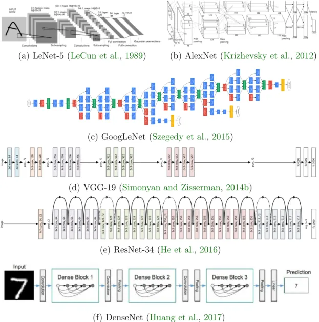
Figure 2.3: Common neural network architectures.

Now we briefly overview the commonly used neural network architectures for image classification and face recognition tasks.

Common Neural Network Architectures. Image classification is commonly used for investigating efficiency/quality trade-offs of ConvNets in computer vision community. Below we discuss the most popular networks.

LeNet. LeNet (LeCun et al., 1989) was the first convolutional neural network for classification of hand-written digits. LeNet is a 7-level convolutional network, it

(44)

consists of two convolutional layers with sigmoid non-linearity activation functions, two pooling layers and a fully connected layer, see Figure2.3a.

AlexNet. AlexNet (Krizhevsky et al., 2012) won the ILSVRC 2010 competition on the large-scale ImageNet dataset (Russakovsky et al.,2015) by reducing the top-5 error from 26% to 15.3%. AlexNet is composed of 5 convolutional layers followed by 3 fully connected layers, see Figure 2.3b. AlexNet is very similar to LeNet but was stacked with more layers to obtain a deeper network and also with more filters per layer. They replaced the sigmoid with ReLU activations.

GoogLeNet.GoogLeNet (Szegedy et al.,2015) won the ILSVRC 2014 competition by reducing the top-5 error to 6.67%. In GoogLeNet, the authors proposed the inception module. The inception module performs convolution on an input with several very small convolutions (1x1, 3x3, 5x5) in order to drastically reduce the number of parameters. GoogLeNet is composed of 22 layers, see Figure2.3c. Further, in GoogLeNet the authors propose for the first time a structured approach of stacking uniform modules.

VGG. VGG (Simonyan and Zisserman, 2014b) consists of 16 to 19 convolutional layers, and is similar to AlexNet. In difference to AlexNet, the author use only 3x3 convolutions uniformly throughout the architecture, see Figure2.3d.

ResNet.ResNet (He et al.,2016) won the ILSVRC 2015 competition by achieving a top-5 error rate of 3.57% which beats human-level performance. In ResNet, the authors introduced a novel architecture with skip connections or residual connec-tions. Skip connections are also known as gated recurrent units and share a lot of relevance from Recurrent Neural Networks (RNNs), see Figure 2.3e. ResNet has lower complexity than VGG architectures.

DenseNet. DenseNet (Huang et al., 2017) is a variant of ResNet. In DenseNet, there is a dense connectivity that directly connects the output of any layer to all subsequent layers within a module. This encourages feature re-use and and makes the network simpler and highly parameter efficient, see Figure 2.3f.

Face Recognition Networks. Another important application, where ConvNets have been very well deployed is for face recognition, where the general task is to identify faces present in images and videos.

(45)

2.2.4 _{Convolutional Neural Network (CNN)} 19

(a) FaceNet (Schroff et al., 2015)

(b) DeepFace (Taigman et al., 2014)

(c) VGGFace (Parkhi et al.,2015). Image source: Google search.

Figure 2.4: Common face recognition neural network architectures.

FaceNet. FaceNet (Schroff et al., 2015) is a convolutional neural network for tasks such as face recognition, verification and clustering. FaceNet directly learns a mapping from face images to a compact Euclidean space. To train the network, the authors use triplet loss with anchor, positive and negative examples, see Figure 2.4a.

DeepFace. DeepFace (Taigman et al., 2014) is also a deep neural network for the task of face recognition. It employs a nine-layer neural net. DeepFace is trained using a dataset of 4 million facial images belonging to around four thousand people. The model is trained using cross-entropy loss. The conventional pipeline of DeepFace consists of four stages: detect, align, represent, and classify to achieve the face recognition, see Figure 2.4b.

VGGFace.VGGFace (Parkhi et al.,2015) is based on the VGG CNN architecture and VGGFace2 (Cao et al.,2018) is based on the ResNet CNN architecture. Both face

(46)

recognition models are trained on a large scale face dataset: with 2.6 million images of

∼2,600 subjects (VGGFace), and 3.31 million images of 9,131 subjects (VGGFace2). To train the network, the authors use cross-entropy loss, see Figure2.4c. The models are freely available to the research community, unlike FaceNet and DeepFace which are not available publicly. In this thesis, we use VGGFace and VGGFace2 as the base model to extract face features.

Next we discuss the datasets and evaluation metrics used in this thesis.

2.3 Datasets

We provide a short description and notation of datasets repeatedly in this thesis. When referring to a specific episode, we stick to the scheme“[dataset]-[season][episode]”.

We conduct experiments on three challenging face clustering datasets, namely The Big Bang Theory (BBT) (Wu et al.,2013a;Zhang et al.,2016a),Buffy - The Vampire Slayer (BF) (Zhang et al., 2016b), and Harry Potter 1 (ACCIO) (Ghaleb et al., 2015).

We follow the protocol used in several recent video face clustering works (Cinbis et al.,2011;Wu et al., 2013b;Zhang et al.,2016a,b) that focus on improving feature representations for video-face clustering. First, they assume the number of main characters/clusters is known. Second, as the labels are obtained automatically, we learn episode specific embeddings. We also use the same number of characters as previous methods (Zhang et al.,2016a,b), however, it is important to note that we do not discard tracks/faces that are small or have large pose variation. We use the face tracks released by Bäuml et al. (2013) that incorporate several detectors to encompass all pan angles and in-plane rotations up to 45 degrees. Tracks are created via an online tracking-by-detection scheme with a particle filter.

Below we present key information about the datasets. In particular, note that previous works use much smaller datasets. Additionally, it is important to note that different characters have wide variations in the number of tracks, indicated by the cluster skew between largest class (LC) to smallest class (SC).

(47)

2.3.1 _{The Big Bang Theory} 21

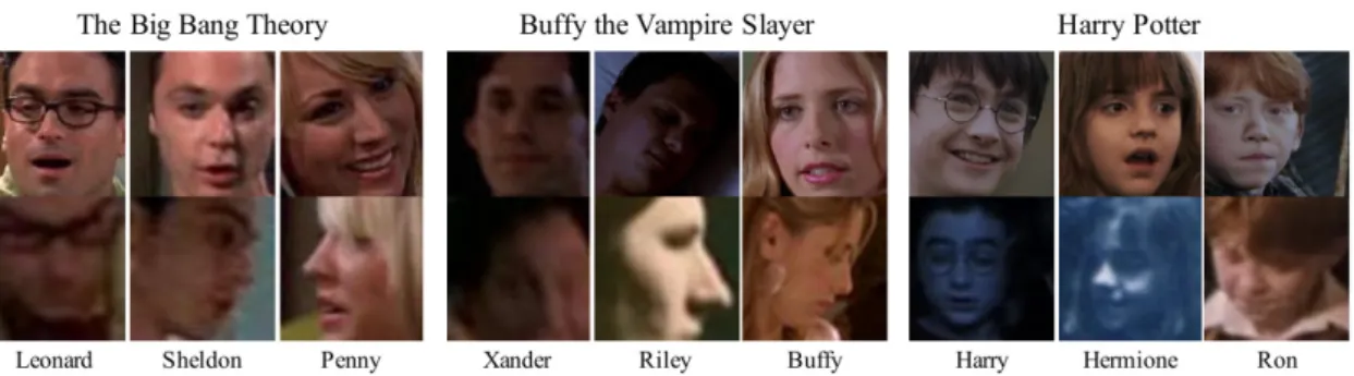
Figure 2.5: Example images for a few characters from our dataset. We show one easy sample and one difficult sample. The extreme variation in illumination, pose, resolution, and attributes (spectacles) make the datasets challenging.

2.3.1 The Big Bang Theory

The first dataset we evaluate is The Big Bang Theory (BBT) (Bäuml et al., 2013; Zhang et al., 2016a), containing face-tracks from the first six episodes of the first season. Traditionally, publications evaluating on BBT use the very first episode for reporting their performance. Since most scenes in BBT are set indoors with studio-lighting, the face-tracks are generally cleaner than in other datasets. There are five main characters, namely Sheldon, Leonard, Penny, Raj and Howard. Kurt is a sixth named character who does not count as a main character. We use the main characters for evaluation unless stated otherwise and discard all face-tracks of unknown characters, face-tracks labeled as false-positives and face-tracks containing track-switches (i.e. the track jumps from one character to another without interruption). Other works (Cinbis et al.,2011; Wu et al.,2013b; Xiao et al., 2014;Zhang et al., 2016a) use fewer tracks; many profile tracks were removed. Table2.1 shows statistics from BBT and exemplary faces can be found in Figure 2.5.

2.3.2 Buffy - The Vampire Slayer

Buffy - The Vampire Slayer (BF) is a TV series about vampires, and thus naturally contains many shots in the dark as well as action shots including motion blur or obstructed faces. The dataset (Bäuml et al., 2013; Zhang et al., 2016b) contains the first six episodes of the fifth season. The episode used for evaluation in other works is the second episode, i.e. BF-0502. There are a total of six main characters: Xander, Buffy, Dawn, Anya, Willow and Giles. Another twelve named characters exist. Similar to BBT, we use all tracks of the main characters and discard all other

(48)

Table 2.1: Statistics for each episode of The Big Bang Theory (Bäuml et al.,2013; Tapaswi et al.,2012;Wu et al., 2013a; Zhang et al., 2016a) (5 main characters), Buffy (Bäuml et al.,

2013; Zhang et al., 2016b) (6 main characters) and ACCIO (Ghaleb et al., 2015) (35 main characters). #TR and #FR is the number of face-tracks and total faces. #Overlaps is the number of tracks that overlap in time. LC/SC indicates the largest and smallest ground truth cluster with non-main characters removed. (Cinbis et al.,2011;Wu et al.,2013a,b;

Xiao et al.,2014;Zhang et al.,2016a) use fewer tracks (last column).

This work Previous work

Dataset #TR (#FR) LC/SC (%) #Overlaps #TR (#FR) BBT-0101 644 (41220) 39.3 / 4.0 313 182 (11525) BBT-0102 613 (32513) 35.1 / 8.6 302 — BBT-0103 530 (30626) 44.0 / 7.7 145 — BBT-0104 449 (27856) 42.1 / 8.5 160 — BBT-0105 404 (26418) 34.4 / 5.7 154 — BBT-0106 623 (40713) 31.3 / 13.6 443 — BF-0501 552 (37758) 42.6 / 5.1 132 — BF-0502 568 (39263) 34.0 / 5.9 173 229 (17337) BF-0503 806 (40546) 30.9 / 1.9 211 — BF-0504 288 (24429) 57.4 / 3.6 44 — BF-0505 543 (34918) 53.7 / 4.1 91 — BF-0506 535 (29340) 31.2 / 8.6 232 — ACCIO 3243 (166885) 30.7 / 0.06 1799 3243 (166885)

tracks in the dataset. Again, previous works (Cinbis et al., 2011; Wu et al., 2013b; Xiao et al., 2014; Zhang et al., 2016a) have evaluated on a smaller subset of the dataset containing less face-tracks of the main characters. In Table 2.1 statistics from each episode of BF are shown. Figure2.5 provides examples.

2.3.3 Harry Potter 1

The final dataset on which we evaluate is the first movie from the “Harry Potter” movie series (Ghaleb et al., 2015). Harry Potter 1 (ACCIO) contains a large number of dark scenes and several tracks with non-frontal faces. In the course of the movie the characters appear in many diverse lighting conditions, many of which are in dark, windowless rooms or lit by fire. In contrast to the other two datasets, ACCIO contains many more main characters, namely 35. Many of them never appear on

(49)

2.3.3 _{Harry Potter 1} 23

Figure 2.6: Co-occurrences resulting in temporal cannot-link edges on ACCIO. Brighter cells appear together more often. Table is log-scale. The regularly scaled table only has very few distinguishable cells between Harry, Ron and Hermione.

screen simultaneously as can be seen in the co-occurrence matrix in Figure 2.6. This implies that there is no cannot-link edge between these characters.

The difference in percentage of face-tracks belonging to the most frequently occurring character (Harry Potter) and the least frequently occurring character is two orders of magnitude greater compared to BBT and BF as shown in Table 2.1. Exemplary faces are shown in Figure 2.5.

Further, note that, in accordance with previous literature (Zhang et al., 2016b), for evaluation of ACCIO throughout the thesis, we use 36 and 40 clusters for the 35 main characters.

(50)

2.4 Metrics

Clustering Accuracy.The metric with which we evaluate our performance on BBT and BF is Weighted Clustering Purity (WCP) (Tapaswi et al., 2014b), also known as Clustering Accuracy (ACC) (Zhang et al.,2016b). It is computed by assigning the most common ground truth label within a cluster to all elements in that cluster: As we compare methods that generate equal numbers of clusters (number of main cast), ACC is a fair metric for comparison.

ACC = 1 N |C| X c=1 nc·pc, (2.11)

where N is the total number of tracks in the video, nc is the number of samples in the clusterc, and cluster purity pc is measured as the fraction of the largest number of samples from the same label tonc. |C| corresponds to the number of main cast members, and in our case also the number of clusters.

Additionally, we also report the clustering accuracy for ACCIO.

B3 _measures. _{The metric with which we evaluate our performance on ACCIO is}

BCubed (B3_{) Precision (P), Recall (R) and F-measure (F) (}_{Amigó et al.}_, ₂₀₀₉_;

Bagga and Baldwin, 1998; Moreno and Dias, 2015). We used BCubed metrics in order to have a fair comparison with previous work Zhang et al.(2016b). BCubed metrics (Amigó et al., 2009) is the best suited technique for evaluating clustering performance with imbalanced class distribution. This is becauseB3 _{metrics estimate}

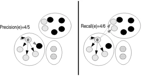
precision and recall for each element of the cluster in comparison to the clustering purity, where the most common ground truth label is assigned to all elements within the cluster for computing purity. For each element e, we can define the correctness of the relation from that element to another elemente0 (Amigó et al.,2009):

(51)

2.4 _Metrics 25

Figure 2.7: Computation ofB3 precision and recall (Amigó et al., 2009) for one element of the datasets. The value for the full dataset is the average over all elements.

Here 1 is the indicator function, L is the ground-truth label of the element, andC is the cluster to which the element is assigned. B3 _{precision and recall over the full}

dataset are then defined as

B3P recision=Avg e [ Avg e0 C(e)=C(e0₎ [Correctness(e, e0)]] (2.13) B3Recall=Avg e [ Avg e0 L(e)=L(e0) [Correctness(e, e0)]] (2.14)

The B3 _{F-Score is the harmonic mean of these values. Figure} _2.7 _{shows how to}

compute recall and precision for one element. The B3 _{score has several advantages}

over WCP discussed in Amigó et al. (2009). We follow the example of previous work (Zhang et al., 2016b) and evaluate with 36 and 40 clusters on the ACCIO dataset.

For all experiments, unless stated otherwise, clustering evaluation is performed at track-level i.e. mean-pool of frames.

(52)