The Markov Chain Monte Carlo Approach to
Importance Sampling in Stochastic Programming
by
Berk Ustun
B.S., Operations Research, University of California, Berkeley (2009)
B.A., Economics, University of California, Berkeley (2009)
Submitted to the School of Engineering
in partial fulfillment of the requirements for the degree of
Master of Science in Computation for Design and Optimization
at the
MASSACHUSETTS INSTITUTE OF TECHNOLOGY
September 2012
c
Massachusetts Institute of Technology 2012. All rights reserved.
Author . . . .
School of Engineering
August 10, 2012
Certified by . . . .
Mort Webster
Assistant Professor of Engineering Systems
Thesis Supervisor
Certified by . . . .
Youssef Marzouk
Class of 1942 Associate Professor of Aeronautics and Astronautics
Thesis Reader
Accepted by . . . .
Nicolas Hadjiconstantinou
Associate Professor of Mechanical Engineering
Director, Computation for Design and Optimization
The Markov Chain Monte Carlo Approach to Importance
Sampling in Stochastic Programming
by
Berk Ustun
Submitted to the School of Engineering on August 10, 2012, in partial fulfillment of the
requirements for the degree of
Master of Science in Computation for Design and Optimization
Abstract
Stochastic programming models are large-scale optimization problems that are used to fa-cilitate decision-making under uncertainty. Optimization algorithms for such problems need to evaluate the expected future costs of current decisions, often referred to as the recourse function. In practice, this calculation is computationally difficult as it involves the evaluation of a multidimensional integral whose integrand is an optimization problem. Accordingly, the recourse function is estimated using quadrature rules or Monte Carlo methods. Although Monte Carlo methods present numerous computational benefits over quadrature rules, they require a large number of samples to produce accurate results when they are embedded in an optimization algorithm. We present an importance sampling framework for multistage stochastic programming that can produce accurate estimates of the recourse function using a fixed number of samples. Our framework uses Markov Chain Monte Carlo and Kernel Den-sity Estimation algorithms to create a non-parametric importance sampling distribution that can form lower variance estimates of the recourse function. We demonstrate the increased accuracy and efficiency of our approach using numerical experiments in which we solve vari-ants of the Newsvendor problem. Our results show that even a simple implementation of our framework produces highly accurate estimates of the optimal solution and optimal cost for stochastic programming models, especially those with increased variance, multimodal or rare-event distributions.
Thesis Supervisor: Mort Webster
Acknowledgments
I would like to take this opportunity to thank my advisors, Mort Webster and Panos Parpas, who have supervised and funded my research at MIT over the past two years. This thesis would not have been possible without their guidance, insight and patience. I would also like to thank Youssef Marzouk, who helped develop and formalize many of the findings that I present in this thesis, as well Bryan Palmintier, who frequently helped resolve all kinds of important problems that I encountered in my research.
Much of this work has involved coding, debugging, computing and waiting... This process was incredibly frustrating at times, but it has certainly been easier in my case thanks to Jeff and Greg who manage the Svante cluster, as well as the anonymous users who post on the CPLEX forums and the StackExchange network. I very much appreciate the fact that these individuals have sacrificed their time and energy to solve problems that, quite frankly, did not affect them in any way. I look forward to the day that I can help others as selflessly as they have helped me.
Looking back at these past two years at MIT, I believe that I have been very fortunate to have been admitted to the CDO program, but even more fortunate to have Laura Koller and Barbara Lechner as my academic administrators. Their support has been invaluable, and I cannot fathom how I could have completed this degree without them.
Contents
1 Introduction 13
2 Background 17
2.1 Modeling Decision-Making Problems using SP . . . 18
2.2 Solving SP Models with Decomposition Algorithms . . . 19
2.2.1 Representing Expected Future Costs with the Recourse Function . . . 19
2.2.2 Approximating the Recourse Function with Cutting Planes . . . 20
2.2.3 Stopping Procedures . . . 21
2.2.4 Overview of Decomposition Algorithms . . . 22
2.3 Using Monte Carlo Methods in Decomposition Algorithms . . . 23
2.4 The Impact of Sampling Error in Decomposition Algorithms . . . 24
2.5 Reducing Sampling Error through Variance Reduction . . . 26
2.5.1 Stratified Sampling . . . 27
2.5.2 Quasi-Monte Carlo . . . 27
2.5.3 Importance Sampling . . . 28
2.5.4 IDG Importance Sampling . . . 30
3 The Markov Chain Monte Carlo Approach to Importance Sampling 33 3.1 Foundations of the Markov Chain Monte Carlo Approach to Importance Sam-pling . . . 34
3.1.1 The Zero-Variance Distribution . . . 34
3.1.2 Overview of MCMC Algorithms . . . 35
3.2 The Markov Chain Monte Carlo Approach to Importance Sampling . . . 37
3.3 MCMC-IS in Practice . . . 40
3.4 MCMC-IS in Theory . . . 43
4 Numerical Experiments on Sampling Properties 45 4.1 The Newsvendor Model . . . 46
4.1.1 A Simple Two-Stage Model . . . 46
4.1.2 A Multidimensional Extension . . . 46
4.1.3 A Multistage Extension . . . 47
4.2 Experimental Setup . . . 48
4.2.1 Experimental Statistics . . . 48
4.2.2 Implementation . . . 48
4.3 Sampling from the Important Regions . . . 49
4.4 The Required Number of MCMC Samples . . . 52
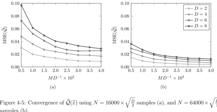
4.4.1 The Curse of Dimensionality . . . 53
4.5 The Acceptance Rate of the MCMC Algorithm . . . 55
4.6 Sampling from Bounded Regions . . . 58
4.7 Choosing Kernel Functions and Bandwidth Estimators in the KDE Algorithm 62 4.8 Comparison to Existing Variance Reduction Techniques . . . 63
4.8.1 Comparison to IDG Importance Sampling . . . 63
4.8.2 Comparison to Other Variance Reduction Techniques . . . 66
5 Numerical Experiments on Performance in Decomposition Algorithms 69 5.1 Experimental Setup . . . 70
5.1.1 Experimental Statistics . . . 70
5.1.2 Implementation . . . 71
5.2 Impact of MCMC-IS Estimates in a Decomposition Algorithm . . . 72
5.3 Impact of MCMC-IS Estimates in Stopping Tests . . . 74
5.4 Computational Performance of MCMC-IS in Multistage SP . . . 78
List of Figures
2-1 A valid sampled cut. . . 25 2-2 An invalid sampled cut. . . 25 2-3 Cross section of points from a Halton sequence (green) and a Sobol sequence
(blue). . . 28 2-4 Cross section of points from a randomized Halton sequence (green) and a
randomized Sobol sequence (blue). . . 28 3-1 Laplacian (green), Gaussian (red) and Epanetchnikov (blue) kernels functions. 37 4-1 Location of samples produced by MCMC-IS and CMC for a Newsvendor
model paired with a lower-variance lognormal distribution. . . 51 4-2 Location of samples produced by MCMC-IS and CMC for a Newsvendor
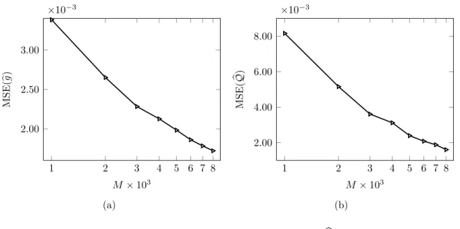
model paired with a multimodal rare-event distribution. . . 51 4-3 Convergence of bgM (a) and Qb(bx) (b). . . 53 4-4 Contours ofg* (a) andbgM for different values of M (b)-(d). . . 54
4-5 Convergence of Qb(bx) using N = 16000×
q D
2 samples (a), and N = 64000×
q D
2 samples (b). . . 55
4-6 Convergence ofQb(bx) by to the step-size of random-walk Metropolis-Hastings MCMC algorithm for a Newsvendor model paired with a lower-variance log-normal distribution (a), a higher-variance loglog-normal distribution (b), and a multimodal rare-event distribution (c). . . 59 4-7 Convergence of Qb(bx) for MCMC-IS and MCMC-IS HR for a Newsvendor
model paired with a lower-variance lognormal distribution (a), a higher-variance lognormal distribution (b) and a multimodal rare-event distribution (c). . . . 61
4-8 Convergence of Qb(bx) for various kernel functions (a) and bandwidth estima-tors (b). . . 63 4-9 Error in IDG estimates ofQb(bx) for a Newsvendor model paired with a
lower-variance lognormal distribution (a) and a higher-lower-variance lognormal distribu-tion (b). The value of p determined the boundaries Ω of the grid used to represent Ξ; higher values of pcorrespond to wider boundaries. . . 64 4-10 Error in IDG (a) and MCMC-IS (b) estimates of the recourse functionQb(bx) for
a multidimensional Newsvendor model paired with a lower-variance lognormal distribution. . . 65 4-11 Mean-squared error and standard error in estimates ofQb(bx) for a Newsvendor
model produced by MCMC-IS and other variance reduction techniques; the model is paired with a lower-variance lognormal distribution in (a)-(b), a higher-variance lognormal distribution in (c)-(d), and a multimodal rare-event distribution in (e)-(f). . . 67 5-1 Error in the estimates of the optimal solution and optimal cost for a
Newsven-dor model produced by MCMC-IS and other variance reduction techniques; the model is paired with a lower-variance lognormal distribution in (a)-(b), a higher-variance lognormal distribution in (c)-(d), and a multimodal rare-event distribution in (e)-(f). . . 73 5-2 Stopping test output from Newsvendor model paired with a lower-variance
lognormal distribution (left column), a higher-variance lognormal distribution (middle column), and a multimodal rare-event distribution (right column); we vary the value ofαin the stopping test between 0.5 - 0.9 and plot the standard error in estimates (top row), the # of cuts until convergence (second row), and the error in the estimated optimal cost (third row), and the error in the estimated optimal solution (bottom row). . . 77 5-3 (a) Complexity of SDDP with MCMC-IS grows quadratically with the
num-ber of dimensions. (b) Estimated optimal cost remains within 1% even for problems with a large number of time periods. . . 79
List of Tables
3.1 Bandwidth estimators for KDE algorithms. . . 38 4.1 Parameters of demand and sales price distributions for the Newsvendor model. 47 4.2 Sampling statistics reported in Chapter 4. . . 49 4.3 Sampling methods covered in Chapter 4. . . 50 4.4 Acceptance rates and step-sizes of MCMC algorithms used in MCMC-IS. . . 57 5.1 Sampling statistics reported in Chapter 5. . . 70 5.2 Sampling methods covered in Chapter 5. . . 71 5.3 Stopping test output from a Newsvendor model paired with a lower-variance
lognormal distribution. . . 75 5.4 Stopping test output from a Newsvendor model paired with a higher-variance
lognormal distribution. . . 76 5.5 Stopping test output from a Newsvendor Model paired with a multimodal
Chapter 1
Introduction
Stochastic programming (SP) models are large-scale optimization problems that are used to facilitate decision-making under uncertainty. Optimization algorithms for such problems require the evaluation of the expected future costs of current decisions, often referred to as the recourse function. In practice, this calculation is computationally difficult as it involves a multidimensional integral whose integrand is an optimization problem. Subsequently, many SP practitioners estimate the value of recourse function using quadrature rules ([30]) or Monte Carlo (MC) methods ([5] and [36]).
MC methods are an appealing way to estimate the recourse function in SP models because they are well-understood, easy to implement and remain computationally tractable for large-scale problems. Unfortunately, MC methods also produce estimates that are subject to sampling error, which can compound across the iterations of an optimization algorithm and produce highly inaccurate solutions for SP models. It is true that one can reduce the sampling error in MC estimates of the recourse function by increasing the number of samples used in an MC approach. In the context of SP, however, the number of samples that can be used to build an MC estimate of the recourse function is generally limited by the fact that each sample requires the solution to a separate optimization problem. As a result, MC methods are often paired with a variance reduction technique to reduce the sampling error in MC estimates of the recourse function without having to increase the number of samples. This thesis focuses on a variance reduction technique known as importance sampling, which can dramatically reduce the sampling error of MC estimates by using an importance
sampling distribution to generate samples from regions that contribute most to the value of the recourse function. Although many distributions can achieve variance reduction through importance sampling, the most effective importance sampling distributions are typically crafted in order to exploit prior knowledge about the SP model. In light of this fact, the primary contribution of this thesis is an importance sampling framework that can reduce the sampling error in MC estimates without requiring the need to specify an importance sampling distribution beforehand.
Our framework, which we refer to as the Markov Chain Monte Carlo Approach to Im-portance Sampling (MCMC-IS), is based on an imIm-portance sampling distribution that is designed to produce MC estimates with zero variance ([2]). Although this zero-variance dis-tribution cannot be used in practice, it is often used to guide the design of effective impor-tance sampling distributions. Accordingly, our framework exploits the fact the zero-variance distribution is known up to a normalizing constant in order to build an approximation to the zero-variance distribution for importance sampling. In particular, MCMC-IS uses a Markov Chain Monte Carlo (MCMC) algorithm to generate samples from the zero-variance distribution, and then uses a Kernel Density Estimation (KDE) algorithm to reconstruct an approximate variance distribution from these samples. With this approximate zero-variance distribution at hand, MCMC-IS then generates a new, larger set of samples and constructs an importance sampling estimate of the recourse function which has lower vari-ance, and thus lower sampling error.
MCMC-IS has several benefits as a sampling framework: it is non-parametric, in that it does not require users to specify a family of importance sampling distributions; flexible, in that it can accommodate a wide array of MCMC and KDE algorithms; and robust, in that it can generate good results for probability distributions that are difficult to work with using existing sampling methods. It follows that MCMC-IS is advantageous in the context of SP because it can produce accurate estimates of the recourse function and improve the accuracy of output from an optimization algorithm. However, MCMC-IS is also beneficial in this context because can produce lower-variance estimates of the recourse function that improves the performance of stopping tests that assess the convergence of optimization algorithms. Moreover, MCMC-IS is well-suited for SP models because the computational overhead
re-quired to build an approximate zero-variance distribution is negligible in comparison to the computational overhead required to evaluate the recourse function in these models.
In this thesis, we demonstrate the performance of MCMC-IS using a series of numerical experiments based on a Newsvendor model. Our results show that MCMC-IS performs well in comparison to existing various reduction techniques, such as stratified sampling methods, Quasi-Monte Carlo methods and an early importance sampling technique developed in [7] and [20]. In particular, we show that MCMC-IS significantly outperforms the these tech-niques when the uncertainty is modeled using a higher variance, rare-event or multimodal distribution. Even as our numerical experiments illustrate the computational performance of the MCMC-IS framework when it is embedded in the Stochastic Dual Dynamic Programming (SDDP) algorithm from [31], we stress that MCMC-IS can yield similar benefits in other algorithms that involve expected-value optimization, such as the sample average approxima-tion method ([36]), stochastic decomposiapproxima-tion ([17]), progressive hedging ([34]), variants of Benders’ decomposition ([5]) and approximate dynamic programming algorithms ([32]).
Although both MCMC and KDE algorithms have received considerable attention in the literature, they have not been previously combined in an importance sampling framework such as MCMC-IS, or applied to solve SP models. Nevertheless, the findings in this the-sis build on existing research on the application of variance reduction techniques for MC methods in SP: Quasi-Monte Carlo methods were studied in [21] and in [10]; control variates were proposed in [37] and in [16]; a sequential sampling algorithm was proposed in [3]; an alternative importance sampling technique for SP was first developed in [7] and [20]. A computational assessment of conditional sampling, antithetic sampling, control variates and importance sampling appeared in [16]. Similarly, Quasi Monte Carlo methods and Latin Hy-percube Sampling were compared in [19]. The link between sampling error of MC estimates and the solution quality of SP models was discussed in [23].
The remaining parts of this thesis are structured as follows. In Chapter 2, we provide a brief overview of SP models, illustrate how decomposition algorithms can produce inaccurate results when paired with an MC method, and provide an overview of variance reduction techniques to remedy this problem. In Chapter 3, we introduce MCMC-IS and provide a detailed overview of its practical and theoretical aspects. In Chapters 4 and 5, we present the
results of numerical experiments based on a Newsvendor model to illustrate the sampling properties of MCMC-IS, and highlight its benefits when it is used with a decomposition algorithm. Finally, we summarize our contributions and outline directions for future research in Chapter 6.
Chapter 2
Background
In this chapter, we explain how to model problems in decision-making under uncertainty using an SP model (Section 2.1). We then show how to simplify this model using a recourse function to represent the expected future costs of current decisions (Section 2.2.1). Next, we provide insight as how to solve this model using a decomposition algorithm (Sections 2.2.2 -2.2.4), and we discuss the merits of estimating the value of recourse function in decomposition algorithms through an MC method, especially in the context of large-scale problems. We then present a simple example to illustrate how sampling error of MC estimates of the recourse function can significantly affect the output from a decomposition algorithm (Section 2.3). Given the relationship between the sampling error of MC estimates of the recourse function and the accuracy of the output from decomposition algorithms, we end this chapter with an overview of variance reduction techniques that can decrease the impact of sampling error in MC estimates (Section 2.5).
2.1
Modeling Decision-Making Problems using SP
A multistage stochastic linear program is an optimization problem that minimizes the ex-pected cost of sequential decisions in an uncertain setting. Given a fixed time horizon T, a set of decisions vectorsx1, . . . , xT, and a set of random variablesξ2, . . . , ξT, we can formulate
the deterministic equivalent of a T-stage stochastic linear program as
z∗ = min x1,...,xT cT1x1 +E hXT t=2 ct(ξt)Txt i s.t. A1x1 =b1 At(ξt)xt=bt(ξt)−Wt(ξt)xt−1 t= 2, . . . , T xt≥0 t= 1, . . . , T (2.1)
We assume thatct ∈Rnt,At∈Rnt×mt,Wt ∈Rnt−1×mt,bt∈Rmt×1. The components of these
parameters are deterministic for t= 1, but may be random fort = 2, . . . , T. We refer to the set of all random components of the parameters at stage t using a Dt-dimensional random
vectorξt, and denote its joint probability density function, cumulative distribution function
and support as ft,Ft and Ξt respectively. In the context of two-stage problems, we simplify
our notation by dropping the time index t, using an (N1×1) vector xto represent decisions
in the first stage and an (N2×1) vector y to represent decisions in the second stage.
The deterministic equivalent formulation of a multistage stochastic linear program models the uncertainty in a decision-making problem as a scenario-tree, which implies that the solution to the linear program in (2.1) represents the optimal decisions for every branch of this tree. Although this approach is straightforward and comprehensive, it is rarely used in practice because the linear program in (2.1) grows exponentially with the number of stages and random outcomes of the underlying decision-making problem. In fact, using the deterministic equivalent to model a decision-making problem with T stages and K random outcomes per stage involves a linear program with O(TK) variables and constraints. This
represents a significant computational burden in the context of large-scale problems in terms of the memory that is required to store the linear program, and the processing power that is required to solve within an acceptable timeframe.
2.2
Solving SP Models with Decomposition Algorithms
2.2.1 Representing Expected Future Costs with the Recourse Function
Decomposition algorithms are a set of optimization algorithms that are designed to solve SP models in a computationally tractable manner. In contrast to the comprehensive determin-istic equivalent approach in (2.1), decomposition algorithms isolate the costs and decisions associated with each stage of the decision-making problem into T nested linear programs, which we denote as LP1, . . . ,LPT. In this case, LP1 is expressed as,
z∗ = min x1 c1x1+Q1(x1) s.t. A1x1 =b1 x1 ≥0 (2.2)
and LPt for t= 2. . . T are expressed as,
Qt−1(bxt−1, ξt) = min
xt ct(ξt)xt+Qt(xt)
s.t. At(ξt)xt=bt(ξt)−Wt(ξt)bxt−1
xt≥0
(2.3)
The decomposed formulation in (2.2) and (2.3) captures the sequential and uncertain structure of the decision-making process as LP2, . . . ,LPT depend on the previous stage
deci-sionxbt−1 and a realization of the uncertainty ξt. We formalize this dependence by
represent-ing the optimal cost of LPtfort = 2. . . T using the functionQt−1(bxt−1, ξt). We note that we
set QT(xT, ξT) ≡ 0 without loss of generality because we assume that our decision-making
problem ends after T stages.
The decomposition formulation in (2.2) and (2.3) frames the optimal decision at each time period as a decision that balances present costs and expected future costs. In particular, the optimal decision at stage t minimizes the sum of present costs at stage t, which are expressed as ct(ξt)xt, and expected future costs at stages t+ 1, . . . , T, which are expressed
using a functionQt(xt) that omits the expectation operator for clarity. The function Qt(xt)
is referred to as the recourse function, and it is defined as
Qt(xt) =E[Qt(xt, ξt+1)] =
Z
Ξt
Qt(xt, ξt+1)ft+1(ξt+1) (2.4)
2.2.2 Approximating the Recourse Function with Cutting Planes
The recourse function Qt(xt) defined in (2.4) represents the expected value of a linear
pro-gram with multiple random parameters. As a result, its value can only be determined by evaluating a multidimensional integral whose integrand is a linear program. Given the computational burden involved in evaluating multidimensional integrals, let alone linear programs, the recourse function should be approximated using few functional evaluations in order to solve SP models in a computationally tractable way.
Decomposition algorithms achieve this goal by constructing a piecewise linear approxi-mation to the recourse functionQt(xt) which only requires the evaluation of the
multidimen-sional integral at a limited number of points xt. The resulting approximation is a collection
of supporting hyperplanes to the recourse function at fixed points xt. In the SP literature,
the supporting hyperplanes are referred to as cutting planes or cuts, and the fixed points xt
around which the cuts are built are emphasized using the notation bxt. Given a fixed point b
xt, a cut is a linear inequality defined as,
Qt(xt)≥ Qt(bxt) +∇Qt(bxt)(xt−bxt) (2.5)
In practice, the values of the cut parametersQt(bxt, ξt+1) and∇Qt(bxt, ξt+1) are determined
using the expected values of the optimal dual variables λt+1 from LPt+1. In particular,
Qt(bxt) = E[Qt(bxt, ξt+1)] = E[λTt+1(bt(ξt+1)−Wt(ξt+1)]
∇Qt(bxt) = E[∇Qt(bxt, ξt+1)] = E[λtT+1Wt(ξt+1)]
(2.6)
Given that the linear inequality defined in (2.5) has the same number of variables as LPt, it is
of the recourse functionQt.
We note that the benefit of using the optimal dual variables in constructing the cut parameters is that they can still be determined when LPt+1 is infeasible for a given value of
the previous stage decisionbxt or the uncertain outcome ξt+1. In such cases, a decomposition
algorithm can use any feasible set of dual variables to construct a cut that will prevent infeasible instances of LPt+1. This cut is refered to as a feasibility cut, and it is defined as,
Qt(xt)≥ ∇Qt(xbt)(xt−bxt) (2.7)
2.2.3 Stopping Procedures
A generic iteration of a decomposition algorithm consists of constructingT−1 cuts to support the recourse functions Q1, . . . ,QT−1 at a set of fixed values bx1, . . . ,bxT−1, and adding these
cuts to the linear programs LP1, . . . ,LPT−1. Assuming that the cut parameters in (2.6)
can be calculated exactly, each cut that is added to LPt improves the approximation of the
recourse function Qt, and brings the estimated values of the optimal decision ˜xt and the
optimal cost ˜ztcloser to their true values x*tandz*t. Although it is impossible to determine
the true optimal cost z* of a multistage SP in a general setting, a decomposition algorithm can produce a lower bound zLB and a upper bound zUB to z*. Given that the value of the
lower bound zLB is monotonically non-decreasing with each iteration and the value of the
upper boundzUB is monotonically non-increasing with each iteration, these bounds can then
be used to stop decomposition algorithms when their difference |zLB−zUB| is smaller than
a user-prescribed tolerance.
The lower bound zLB produced by decomposition algorithms exploits the fact that a
cutting plane approximation of the recourse function consistently underestimates the value of the true recourse function. This is because the approximation is composed of supporting hyperplanes to a convex function. In this case, the convexity of the recourse function is assured as it represents the expected value of a convex function (we note that the cost of a linear program is a convex function, and the expected value operation preserves convexity). As a result, we can obtain a lower bound zLB to the true optimal costz* by considering the
incur in future stages,
zLB = min
x1
c1x1+Qb1(x1) (2.8)
Given that a cutting plane approximation of the recourse function consistently underes-timates expected future costs, it follows that decisions made with this approximate recourse function will be suboptimal. By definition, the true expected cost of these suboptimal de-cisions will exceed the optimal cost of the SP model. In other words, we can obtain an upper bound to the true optimal cost by calculating the true expected cost of the subop-timal decisions that are produced with our current approximation of the recourse function. In the context of a multistage SP, we can calculate the true expected cost of these decisions by calculating the cost associated with each sequence of uncertain outcomes ξi
2, . . . , ξTi, and
forming its expected value. Assuming that there exists K unique sequences of uncertain outcomes, the upper bound can be calculated as
zUB = K X i=1 T X t=1 ct(ξti) ˜xt(ξti)ft(ξti) (2.9) where, ˜ xit(ξti) = arg minct(ξti)xt+Qbt(xit) (2.10)
2.2.4 Overview of Decomposition Algorithms
All decomposition algorithms solve SP models hrough an iterative process that builds cuts around fixed points bxt and adds them to LPt for t = 1, . . . , T −1. The differences between
these algorithms are primarily based in the way that they choose the fixed pointsbxt around
which they build cuts, the number of cuts that they add with each iteration, and whether they keep the cuts, drop them after a fixed number of iterations, or refine them with each iteration. In the context of multistage models, decomposition algorithms can also differ in the order of the stages at which they build the cuts.
Decomposition algorithms that can be characterized using these traits include the Abridged Nested Decomposition algorithm from [9], the Cutting Plane and Partial Sampling algorithm from [6],the ReSa algorithm from [18] and the Stochastic Decomposition algorithm from [17].
In this thesis, we restrict our focus on the SDDP algorithm that is presented in [31] due to its popularity among SP practitioners. The SDDP algorithm uses a greedy procedure to pick the fixed points bxt, adds a single cut to LPt for t= 1, . . . , T −1 at each iteration, and
permanently keeps the cuts that are produced with each iteration.
We refer the interested reader to [24] for a simple theoretical comparison between decom-position algorithms, and to [5] for a comprehensive introduction to the theory and practice of multistage SP.
2.3
Using Monte Carlo Methods in Decomposition Algorithms
The computational bottleneck in solving a multistage stochastic linear program involves calculating the cut parameters in (2.6), as this requires the evaluation of a multidimensional integral whose integrand is a linear program. While the cut parameters are easy to calculate when ξt+1 is a discrete random variable with few outcomes, the calculation is intractable
whenξt+1is high-dimensional, and impossible whenξt+1continuous. Subsequently, many SP
practitioners simplify this calculation by modeling the uncertainty in their decision-making problem using scenario trees.
Scenario trees are discrete in nature, meaning that they either require models that ex-clusively contain discrete random variables, or a discretization procedure that can represent continuous random variables using a finite set of outcomes and probabilities. In the latter case, we note the optimal solution to an SP model in which the continuous random variables are discretized may differ from the optimal solution of an SP model in which the continuous random variables are kept in place. Even in situations where a scenario tree approach can produce accurate solutions, this level of accuracy is difficult to maintain in large-scale prob-lems with multiple random variables and time periods due to the exponential growth in the size of the scenario tree. In such cases, scenario trees impose an unnecessary choice between high-resolution discrete approximations that yield accurate solutions but are difficult to store and solve, and low-resolution discrete approximations that may yield inaccurate solutions but are easier to store and solve.
advantages of this approach are that it can accommodate discrete or continuous random vari-ables, remain computationally tractable for models with a large number of random variables and produce estimates of the recourse function whose error does not depend on the number of random variables in the model. In practice, an MC method involves randomly samplingN
i.i.d. outcomes of the uncertain parametersξ1
t+1. . . ξtN+1, and estimating the expected values
of the cut parameters in (2.6) through the sample averages,
Qt(bxt) ≈ Qbt(xbt) = 1 N N X i=1 Qt(bxt, ξti+1) ∇Qt(bxt) ≈ ∇Qbt(xbt) = 1 N N X i=1 ∇Qt(bxt, ξti+1) (2.11)
Given that the cut parameters in (2.11) are produced by random sampling, it follows that they are subject to sampling error. In turn, the supporting hyperplane that is produced using these parameters is also subject to sampling error. We refer to this supporting hyperplane as a sampled cut, and note that it has the form,
Qt(xt)≥Qbt(bxt) +∇Qbt(bxt)(xt−bxt) (2.12)
2.4
The Impact of Sampling Error in Decomposition Algorithms
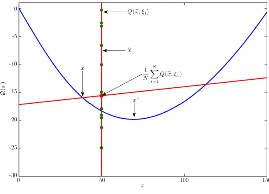
In comparison to the exact cut in (2.5), the sampled cut in (2.12) may produce an invalid approximation of the recourse function. We illustrate this phenomenon in Figures 2-1 and 2-2, where we plot sampled cuts that are produced when a crude MC method is paired with a decomposition algorithm to solve a simple two-stage Newsvendor model. We note that the parameters of this model are specified in Section 4.1.1.
Both cuts in this example were constructed using N = 50 samples. For clarity, we plot a subset of the sample values Q(bx, ξi) fori= 1, . . . , N along the vertical line ofbx, as well as
their sample average N1 PNi=1Q(bx, ξi). In Figure 2-1, we are able to generate a valid sampled
cut, which is valid because it underestimates the true recourse function Q(x) at all values of
x. However, it is possible to generate a sampled cut that in some regions overestimates, and in other regions underestimates the true recourse functionQ(x). We illustrate this situation
x Q ( x ) 1 N N X i=1 Q(bx, ξi) ˜ x 0 -5 -10 -15 -20 -25 -30 0 50 100 150 x∗ b x Q(bx, ξi)
Figure 2-1: A valid sampled cut.
x Q ( x ) x∗ b x 1 N N X i=1 Q(bx, ξi) Q(x, ξb i) 0 -5 -10 -15 -20 -25 -30 0 50 100 150
in Figure 2-2, where the sampled cut excludes the true optimal solution at x∗ ≈ 69 with
z∗ ≈ −20. Assuming that the decomposition algorithm will only generate valid sampled cuts until it converges, the resulting estimates of x∗ and z∗ will be ˜x ≈ 38 and ˜z ≈ −15, corresponding to errors of 80% and 25% respectively. We note that the optimal solution x∗
corresponds to the value ofxthat minimizes the sum of the first-stage costs and the recourse function, and not the value of xthat minimizes the recourse function (although these values appear to be very close to each other in Figures 2-1 and 2-2).
Even in cases where sampling error in MC estimates of the cut parameters is negligible, its presence can have a significant impact on the final values of the optimal solution and optimal cost that are produced from a decomposition algorithm. This is because multiple quantities that affect the final output in a decomposition algorithm also depend on the cut parameters, such as the values of the lower bound zLB and the upper bound zUB that are
used to stop the algorithm. In this case, the presence of sampling error means that these quantities are no longer deterministic values but random distributed estimates and a suitable statistical procedure is required in order to stop the algorithm. As we demonstrate in Section 5.3, a poorly designed procedure in such situations may stop decomposition algorithm before it has converged, and thereby result in highly inaccurate estimates of the optimal solution and the value.
2.5
Reducing Sampling Error through Variance Reduction
It is well-known that the sampling error in MC estimates of the cut parameters can be expressed as, SE(Qbt(bxt)) = q Var[Qbt(bxt)] = σQt(bxt) √ N SE(∇Qbt(bxt)) = q Var[∇Qbt(bxt)] = σ∇Qt(bxt) √ N (2.13)
where σQt(xbt and σ∇Qt(bxt) represent the true standard deviation of the recourse function
and its gradient at the fixed point bxt respectively. Although (2.13) implies that we can
reduce the sampling error of MC estimates by increasing the number of samples, theO(√1
convergence rate implies that we have to solve four times as many linear programs in order to halve the sampling error of the cut parameters. Given the time that is required to solve a linear program within a large-scale multistage SP model, such an approach is simply not tractable. As a result, MC methods are typically paired with a variance reduction technique that can reduce the sampling error of MC estimates by either improving the convergence rate or reducing the underlying variance of the model.
Variance reduction techniques have generated much interest due to the application of MC methods across numerous fields; we refer the interested reader to [12], [22] and [25] for an introductory overview of these techniques.
2.5.1 Stratified Sampling
Stratified sampling techniques are a set of variance reduction techniques that first split the support Ξ of a random variable ξ into K strata, and generate samples from each of the K
strata. This approach ensures that the samples are randomly distributed while achieving some variance reduction by spreading samples across the entire sample space. WhenK =N
strata are used, the stratified sampling technique is referred to as Latin Hypercube Sampling (LHS), and it produces estimates whose sampling error converges at a rate of O(√1
N) albeit
within a constant factor of traditional MC methods. We note that this convergence rate is slow in comparison to state-of-the-art stratified sampling techniques, which can increase the rate by allocating the N samples in proportion to the variance of each K strata. We recommend [26] and [40] for a more detailed overview of stratified sampling and LHS.
2.5.2 Quasi-Monte Carlo
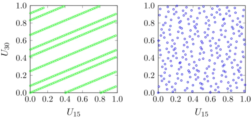
Quasi Monte Carlo (QMC) methods are a set of variance reduction techniques that reduce the sampling error in MC estimates by using a deterministic sequence of points that is uniformly distributed across multiple dimensions. Examples of such sequences include Halton and Sobol sequences, whose points are depicted in Figure 2-3.
QMC methods are typically paired with a scrambling algorithm that is specifically de-signed to randomize a particular sequence of points. Popular examples of scrambling algo-rithms include the Owen scrambling algorithm for Sobol sequences, and the Reverse-Radix
0.0 0.2 0.4 0.6 0.8 1.0 0.0 0.2 0.4 0.6 0.8 1.0 U15 U30 0.0 0.2 0.4 0.6 0.8 1.0 0.0 0.2 0.4 0.6 0.8 1.0 U15
Figure 2-3: Cross section of points from a Halton sequence (green) and a Sobol sequence (blue).
2 algorithm for Halton sequences. As shown in Figure 2-4, scrambling randomizes the points from QMC sequences while maintaining their uniformity across each dimension.
0.0 0.2 0.4 0.6 0.8 1.0 0.0 0.2 0.4 0.6 0.8 1.0 U15 U30 0.0 0.2 0.4 0.6 0.8 1.0 0.0 0.2 0.4 0.6 0.8 1.0 U15
Figure 2-4: Cross section of points from a randomized Halton sequence (green) and a ran-domized Sobol sequence (blue).
In the cases that an MC estimate is produced using N randomized points from a QMC method, it has been shown that the sampling error in the estimates converges at an improved rate of O(logN1N.5
0.5(D−1)
) so long as the recourse function is smooth. For a more detailed introduction to QMC methods, we refer the reader to [28] and [29].
2.5.3 Importance Sampling
Importance sampling is a variance reduction technique that aims to reduces the sampling error in MC estimates by generating samples from an importance sampling distribution g, as opposed to the original sampling distribution f. When samples are generated from an
importance sampling distribution g, the recourse function can be calculated as, Q(bx) =Ef[Q(bx, ξ)] = Z Ξ Q(bx, ξ)f(ξ)dξ = Z Ξ Q(bx, ξ)f(ξ)g(ξ) g(ξ)dξ = Z Ξ Q(bx, ξ)f(ξ) g(ξ)g(ξ)dξ = Z Ξ Q(bx, ξ)Λ(ξ)g(ξ)dξ =Eg[Q(bx,Λ(ξ)] (2.14) In (2.14), the function Λ : Ξ→R, Λ(ξ) = f(ξ) g(ξ) (2.15)
is typically refered to as the likelihood function, and it is used to correct the bias that is produced by the fact that we generated samples from the importance sampling distribution
g instead of the original distributionf. Once we select a suitable important sampling distri-bution g, we can generate a set of N i.i.d. samplesξ1, . . . , ξN, and construct an importance
sampling estimate of the recourse function as,
b Q(bx) = 1 N N X i=1 Q(bx, ξi)Λ(ξi) (2.16)
In theory, importance sampling simply reflects a change in the measure with which we compute the recourse function at a fixed pointbx. Accordingly, any distributiongcan be used as an importance sampling distribution as long as the likelihood function Λ is well-defined over the support of f. In other words, the importance sampling distribution g should be chosen so thatg(ξ)>0 at all values ofξ wheref(ξ)>0. When this requirement is satisfied, the sampling error of importance sampling methods also converges at a rate ofO(√1
N), albeit
with a different constant factor than traditional MC methods.
Ideally, an importance sampling distributiong is one that can generate samples at regions where Q(bx)f(ξ) attains high values, which are referred to as the important regions of the
recourse function. Nevertheless, we stress that the importance sampling distributiongshould also be able to evaluate the probability g(ξ) of each sample to a high degree of accuracy. This is because misspecified values of the importance sampling distributiong(ξ) will produce misspecified values of the likelihood Λ(ξ), and produce an importance sampling estimate that is highly biased.
We refer the interested reader to [2] for a more detailed review of importance sampling.
2.5.4 IDG Importance Sampling
Importance sampling was first applied to SP in [7] and [20]. We refer to this importance sampling distribution proposed as the Infanger-Dantzig-Glynn (IDG) distribution. The IDG distribution has been shown to mitigate the issues associated with the use of sampled cuts in decomposition algorithms that we cover in Section 2.3. Unfortunately, the IDG distribution in these papers makes several assumptions which severely limit its applicability to a broad range of SP models.
To begin with, the IDG distribution can only be used in SP models where the uncertainty is modeled using discrete random variables. As a result, any SP model where we can use the IDG distribution for importance sampling is subject to the same computational issues that we attribute to the scenario tree approach in Section 2.3.
Moreover, the IDG distribution assumes that the cost surface Q(bx, ξ) is additively sepa-rable in the random dimensions, meaning that
Q(bx, ξ)≈
D X d=1
Qd(bx, ξd) (2.17)
In SP models where such an approximation does not hold, the sampling error in the IDG estimate will still converges at a rate that is O(√1
N) but with a much larger constant than
traditional MC methods. In such cases, the IDG distribution produces estimates that are have high rates of error.
A final issue with the IDG distribution is that it requires practioners to know or determine the value of random outcomeξwhich minimizes the cost surfaceQ(bx, ξ). In a general setting, the only way to determine the value is to perform an exhaustive search across all the uncertain
outcomes ξ ∈Ξ.
It is true that there exist practical ways to work around these assumptions. However, we note that our numerical experiments in Section 4.8.1 suggest that the performance of the IDG distribution is critically determined by these factors. In turn, there remains a need for an alternative approach importance sampling that does not suffer from such issues for a broader range of SP models.
Chapter 3
The Markov Chain Monte Carlo
Approach to Importance Sampling
In this chapter, we introduce the zero-variance importance sampling distribution (Section 3.1.1) and provide an overview of MCMC algorithms (Section 3.1.2) and KDE algorithms (Section 3.1.3). We then proceed to explain how these algorithms can be combined to build an importance sampling distribution that approximates the zero-variance distribution (Section 3.2) - a procedure that we refer to as the Markov Chain Monte Carlo Approach to Importance Sampling (MCMC-IS). Having introduced MCMC-IS, we present a simple MCMC-IS implementation to illustrate how MCMC-IS can be used in practice (Section 3.3). We end this chapter with a discussion of the theoretical aspects of MCMC-IS where we cover the ingredients of a convergence analysis (Section 3.4).
3.1
Foundations of the Markov Chain Monte Carlo Approach to
Importance Sampling
3.1.1 The Zero-Variance Distribution
Importance sampling is most effective in the context of SP models when the importance sampling distribution g can generate samples from regions that contribute the most to the value of the recourse function Q(bx). In fact, when an importance sampling distribution can generate samples according to the exact importance of each region as,
g∗(ξ) = |Q(bx, ξ)|f(ξ)
Ef[|Q(bx, ξ)|]
(3.1)
then the variance and sampling error of its estimates will be minimized (see [2]). Moreover, if the recourse functionQ(x, ξ)>0 for allξ ∈Ξ, then the importance sampling distribution
g* can produce a perfect estimate of the recourse function with only a single sampleξ 1 as, b Q(bx) = 1 N N X i=1 Q(bx, ξi)Λ(ξi) =Q(bx, ξ1) f(ξ1) g*(ξ 1) =Q(bx, ξ1) f(ξ1) Q(bx, ξ1)f(ξ1) Ef[Q(bx, ξ)] =Ef[Q(bx, ξ)] (3.2)
In light of this fact, the importance sampling distribution g* is often referred to as the
zero-variance importance sampling distribution. The problem with using the zero-variance distributiong* in practice is that it requires knowledge of
Ef[|Q(x, ξ)|], which is the quantity
that we sought to compute in the first place. In turn, we are faced with a ”curse of circularity” in that we can use the zero-variance distributiong* to construct perfect estimates if and only
3.1.2 Overview of MCMC Algorithms
MCMC algorithms are an established set of MC methods that can sample from a distribution which is known up to a normalizing constant. In contrast to other MC methods, MCMC algorithms generate a serially correlated sequence of samples ξ1, . . . , ξM. This sequence
constitutes a Markov chain whose stationary distribution is equal to the distribution that we wish to sample from.
The simplest MCMC algorithm is the Metropolis-Hastings algorithm from [27], which we refer to throughout this thesis and cover in detail in Section 3.3. The Metropolis-Hastings algorithm generates samples from a target distribution g by proposing new samples through a proposal distribution q and accepting each sample as the next state of the Markov chain using a simple accept-reject rule.
In addition, we refer to the Adaptive Metropolis algorithm from [14] in Section 4.5, which uses a random walk distribution as the proposal distribution in the Metropolis-Hastings algorithm and automatically scales the step-size within this distribution. Lastly, we cover the Hit-and-Run algorithm from [39] in Section 4.6, which is designed to generate samples within bounded regions by using an accept-reject approach that resembles the Metropolis-Hastings algorithm.
We note that numerous other MCMC algorithms have been developed for different prac-tical applications, and many of them can be used in the importance sampling framework that we present in this thesis. We refer the interested reader to [1],[11], and [13] for a comprehensive overview of the theoretical and practical aspects of MCMC algorithms.
3.1.3 Overview of KDE Algorithms
KDE algorithms are an established set of techniques that are designed to reconstruct a continuous probability distribution from a finite set of samples. Given a set of aM samples,
ξ1, . . . , ξM, the output of a KDE algorithm is an empirical probability distribution function, b gM(ξ) = 1 M M X i=1 KH(ξ, ξi) (3.3)
where the function KH is referred to as a kernel function, and the matrix H ∈ RD×D
is referred to as the bandwidth matrix. We note that the kernel function KH in (3.3)
determines the probability of the region that surrounds each of the M samples ξ1, . . . ξM
while the bandwidth matrix H determines the width of the region spanned by the kernel function KH at each sample.
In theory, the kernel function KH has to be chosen so that the output from the KDE
algorithm bgM(ξ) is a probability distribution. In the multidimensional case, this requires a function KH such that
KH(·,·)≥0 Z Ξ KH(ξ,·)dξ = 1 Z Ξ ξKH(ξ,·)dξ = 0 Z Ξ ξξTKH(ξ,·)dξ = 0 (3.4)
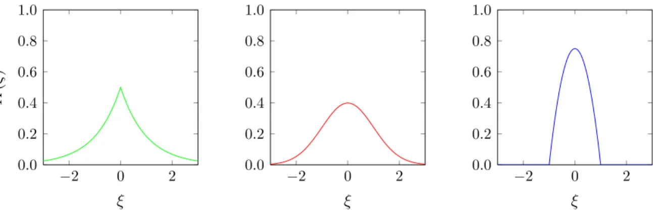
Assuming that these conditions are satisfied, the kernel function is said to be well-behaved, and its shape does not significantly impact the empirical distribution bgM that is produced by a KDE algorithm. In practice, KH is typically set as the product of D one-dimensional
kernel functions K1, . . . , KD that are symmetric around the origin in order to reduce the
computational burden associated with KDE algorithms. Examples of such functions include the Gaussian, Laplacian or Epatchenikov kernel functions, which we plot in Figure 3-1.
In comparison to the impact of the kernel function KH, the bandwidth matrix H can
−2 0 2 0.0 0.2 0.4 0.6 0.8 1.0 ξ K ( ξ ) −2 0 2 0.0 0.2 0.4 0.6 0.8 1.0 ξ −2 0 2 0.0 0.2 0.4 0.6 0.8 1.0 ξ
Figure 3-1: Laplacian (green), Gaussian (red) and Epanetchnikov (blue) kernels functions.
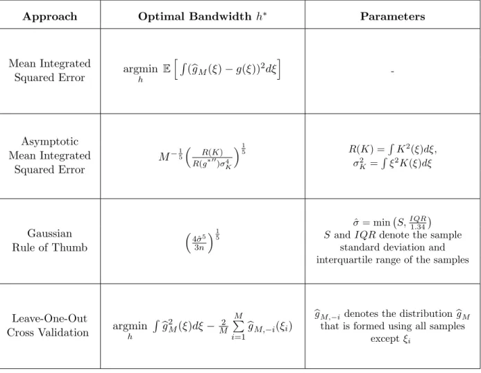
bandwidth matrixH is only required to be symmetric and positive definite, KDE algorithms automate the choice of H through a bandwidth estimator, which determines the value of each entry within H in order to minimize the error inbgM according to different metrics and assumptions. We include an overview of bandwidth estimators in Table 3.1
We note that there exists many different KDE algorithms that can be applied in the importance sampling framework that we present in this thesis. We refer the interested reader to [8], [35] and [38] for an more detailed overview of these algorithms.
3.2
The Markov Chain Monte Carlo Approach to Importance
Sampling
The importance sampling framework that we present in this thesis is motivated by two insights regarding the zero-variance distribution as defined in (3.1).
The first insight is that the zero-variance distribution is known up to a normalizing constantE[|Q(xb, ξ)|]. This implies that we can generate samples from this distribution using an MCMC algorithm. Unfortunately, we cannot use these samples to form a perfect estimate even as they belong to the zero-variance distribution. This is because we still need to evaluate the likelihood of each sample as defined in (2.15). In this case, the likelihood of a sample ξ
is given by,
Λ∗(ξ) = E
f
[|Q(bx, ξ)|]
|Q(bx, ξ)| (3.5)
Approach Optimal Bandwidth h∗ Parameters
Mean Integrated
Squared Error argminh E
h R (bgM(ξ)−g(ξ))2dξi -Asymptotic Mean Integrated Squared Error M−15 R(K) R(g*00)σ4 K 1 5 R(K) = R K2(ξ)dξ, σ2 K = R ξ2K(ξ)dξ Gaussian Rule of Thumb 4ˆσ5 3n 1 5 ˆ σ= min S,IQR1.34 S andIQRdenote the sample
standard deviation and interquartile range of the samples
Leave-One-Out
Cross Validation argminh
R b g2M(ξ)dξ− 2 M M P i=1b gM,−i(ξi) b
gM,−i denotes the distributionbgM
that is formed using all samples exceptξi
samples that we generate from the zero-variance distribution to form a perfect estimate leads us to the second insight: while we cannot use the samples to form an importance sampling estimate, we can use them to reconstruct an approximation of the zero-variance distribution by using a KDE algorithm.
In particular, assuming that we have generated M samples from the zero-variance distri-bution using an MCMC algorithm, we can use a KDE algorithm to reconstruct an approxi-mate zero-variance distributionbgM from these samples. With the approximate zero-variance distributionbgM, we can then produce an importance sampling estimate of the recourse func-tion by generating N additional samples ξ1, . . . , ξN from bgM. As we can now specify both
the original distribution f and the distribution that we used to generate these samples bgM, we can evaluate the likelihood of each sample as,
b
Λ(ξ) = f(ξ)
b
gM(ξ) (3.6)
and form the importance sampling estimate as,
b Q(bx) = 1 N N X i=1 Q(bx, ξi)Λ(ξi) (3.7)
The samples ξ1, . . . , ξN will not originate from the true zero-variance distribution g∗.
Nevertheless, they can still be used to produce an effective importance sampling estimate provided that the KDE algorithm is able to construct abgM that is similar tog∗. Given that the importance sampling distributionbgM will only be an approximation of the zero-variance
distribution g*, it follows that the estimates that are produced through this framework will typically not have zero variance and zero sampling error. Nevertheless, the process of generating samples in regions that contribute most to the value of the recourse function will still lead to importance sampling estimates with low-variance and low-sampling error.
We note that it is possible to generate samples using an MCMC algorithm and then directly construct an importance sampling estimate of the recourse function by using a self-normalized importance sampling scheme, or by using a KDE algorithm to estimate the probability g∗(ξi) for i = 1, . . . , M. We note, however, that resampling from the
approxi-mate zero-variance distributionbgM ultimately produces more accurate importance sampling estimates. This is due to the fact that importance sampling estimates are highly sensitive to the likelihood of each sample, and the resampling process allows us exactly determine the likelihood of each sample used to construct the importance sampling estimate. In con-trast, the use of an MCMC-only approach will approximate the likelihood of each sample and ultimately produce a biased importance sampling estimate. Generating samples from
b
gM is also beneficial in that the samples are independent and the kernel functions are easy to sample from, especially when compared to the computational overhead involved in the MCMC sampling process. In practice, we therefore construct bgM using modest values of M
and then construct an importance sampling estimateQb(bx) using large values of N.
3.3
MCMC-IS in Practice
In this section, we present a simple implementation of MCMC-IS that can be used to generate importance sampling estimates with low sampling error. Our simple implementation uses a Random Walk Metropolis-Hastings algorithm to generate samples from the zero-variance distribution, and a Gaussian product kernel and leave-one-out cross validation bandwidth estimator to construct the approximate zero-variance distribution. We include a step-by-step explanation of how to generate an importance sampling estimate using this implementation in Algorithm 1.
The Metropolis-Hastings algorithm uses a simple accept-reject procedure in order to generate a Markov chain that has (3.1) as its stationary distribution. In the k-th step, the algorithm generates a proposed sample ζk using a proposal distribution q(· | ξk), which
typically depends on the current sample ξk. Together, the proposed sample, the current
sample and the target distribution are used to evaluate an acceptance probability, a(ξk, ζk).
The proposed sample is accepted with probabilitya(ξk, ζk), in which case the Markov Chain
transitions to the proposed sample ξk+1 := ζk. Otherwise, the proposed sample is rejected
with probability 1−a(ξk, ζk), in which case the Markov chain remains at its current sample
ξk+1 :=ξk.
in the Metropolis-Hastings algorithm. This implies that the proposed sampleζk is generated
as,
ζk=ξk+vk (3.8)
where vk is a Gaussian random variable with mean 0 and covariance matrix Σ. When new
samples are proposed through a random walk process, the proposal distribution is symmetric and the acceptance probability can be expressed as,
a(ξk, ζk) = min |Q(bx, ζk)|f(ζk) |Q(bx, ξk)|f(ξk) ,1 (3.9)
In terms of KDE algorithm, we use a Gaussian product kernel function,
KH(ξ, ξi) = D Y k=1 1 √ 2πhk exp (ξk−ξi,k)2 2h2 k (3.10)
where the bandwidth matrix H is a D×D diagonal matrix that contains the bandwidth parameters of each dimension h1, . . . , hD along its diagonal. In this case, we use a
one-dimensional leave-one-out cross validation estimator to estimate the value of the bandwidth parameter hk separately for each dimension k. The exact parameters for this bandwidth
estimator are defined in Table 3.1.
We note that we use this simple MCMC-IS implementation to generate the majority of the numerical results in Chapters 4 and 5 because it is straightforward to implement and does not depend on a restrictive set of assumptions. The quality of numerical results that we achieve with this admittedly simple implementation in these chapters only reinforces the potential of MCMC-IS, as more efficient implementations of MCMC-IS would only further increase the advantages of our framework. It is true that this simple implementation can also lead to certain challenges in practice; we refer to these challenges throughout Chapter 4 and provide recommendations to fix them by using different MCMC and KDE algorithms.
Algorithm 1Markov Chain Monte Carlo Importance Sampling (MCMC-IS)
Require: bx: previous stage decision
Require: M: number of samples to generate using the MCMC algorithm
Require: N: number of samples to generate using the approximate zero-variance distribu-tion
Require: ξ0: starting sample for the MCMC algorithm
Require: q(· |ξk): proposal distribution for the MCMC algorithm
Require: KH: kernel function for the KDE algorithm
Require: H: bandwidth matrix for the KDE algorithm
Step 1: Generate Samples from the Zero-Variance Distribution using MCMC
1: Set k = 0
2: Given the current sample ξk, generate ζk∼q(· | ξk).
3: Generate a uniform random variable u∼U ∈(0,1).
4: Transition to the next sample according to,
ξk+1 = ( ζk if u≤a(ξk, ζk) ξk otherwise where, a(ξk, ζk) = min |Q(bx, ζk)|f(ζk)q(ξk|ζk) |Q(bx, ξk)|f(ξk)q(ζk|ξk) ,1
5: Letk ←k+ 1. Ifk =M then proceed to Step 6. Otherwise return to Step 2.
Step 2: Reconstruct an Approximate Zero-Variance Distribution using KDE
6: For each sample generate from MCMC, reconstruct the approximate zero-variance dis-tribution as, b gM(ξ) = 1 M M X i=1 KH(ξ, ξi)
Step 3: Resample from the Approximate Zero-Variance Distribution to
Form an Importance Sampling Estimate
7: Generate N new samples from bgM and form the importance sampling estimate,
b Q(bx) = 1 N N X i=1 Q(bx, ξi) f(ξi) b gM(ξi)
3.4
MCMC-IS in Theory
The convergence properties of MCMC-IS depend on two sources of error: the first is due to the MCMC algorithm used to generate samples from the zero variance distribution; the second is due to the KDE algorithm used to construct the approximate zero-variance distri-bution.
The main convergence condition in terms of the MCMC algorithm requires that the sam-ples generated by the MCMC algorithm form a Markov chain whose stationary distribution is the zero-variance distribution. This requires the underlying Markov chain in the MCMC process to be irreducible and aperiodic. The irreducibility property means that the chain can eventually reach any subset of the space from any state. The aperiodicity property means that the chain cannot return to a subset of the space in a predictable manner. Formal definitions of these properties can be found in [33]. The first step in the convergence analysis is to show that these two conditions are satisfied.
In order to control the error due to the KDE algorithm, we need to ensure that the number of samples are generated by the MCMC algorithm,M, is large enough, and that the bandwidth, hk, is small enough. In particular, if (M hD)−1 → ∞, h → 0 as M → ∞, and
the distribution is approximated as,
b gM(ξ) = 1 M M X i=1 KH(ξ, ξi) = (M hD)−1 1 M M X i=1 K ξ−ξi h (3.11)
then it has been shown thatbgM will probabilistically converge tog* under the total variation
norm in [8]. Applying this result to MCMC-IS is not straightforward. The complexity stems from the fact that previous convergence proofs for the KDE algorithm assume that samples are generated fromg*, whereas in our framework these samples are generated from a Markov
chain whose stationary distribution is g*.
A final issue that may affect the convergence of MCMC-IS is the fact that the sam-ples generated through the MCMC algorithm are typically correlated, while the samsam-ples used in many treatments of KDE algorithms assume that the samples used to construct a KDE distribution are independent. Our numerical experiments from Chapter 4 suggest that
MCMC-IS can converge even when there is a degree of correlation between MCMC samples. However, we note that there is some theoretical evidence that KDE algorithms do not nec-essarily require the samples independence between the samples. In particular, theoretical results in [15] suggest that KDE algorithms can construct accurate empirical distributions using correlated samples so long as they use a different bandwidth estimator. In cases where this bandwidth estimator is not available, we note that authors of [15] also state that a leave-one-out bandwidth estimator may provide an adequate approximation.
Chapter 4
Numerical Experiments on Sampling
Properties
In this chapter, we illustrate the sampling properties of MCMC-IS using numerical experi-ments based on a Newsvendor model. We begin by introducing a simple Newsvendor model with two random variables and two stages (Section 4.1), and explain how it can be extended to include multiple random variables (Section 4.1.2) and multiple time periods (Section 4.1.3). We then use this model to illustrate how the importance sampling distribution pro-duced by MCMC-IS can sample from important regions of the recourse function (Section 4.3). Next, we demonstrate how the number of MCMC samples used in MCMC-IS can affect the error in MCMC-IS estimates (Section 4.4), and provide insight as to how this relation-ship scales according to the number of random dimensions in the recourse function (Section 4.4.1). In subsequent numerical experiments, we highlight how the acceptance rate of an MCMC algorithm is related to the accuracy and computational efficiency of MCMC-IS esti-mates (Section 4.5), show how to modify MCMC-IS in order to generate samples in bounded regions (Section 4.6), and examine how the choice of kernel functions and bandwidth es-timators in the KDE algorithm of MCMC-IS can impact the estimates that are produced (Section 4.7). We end this chapter with a comparison between MCMC-IS and other variance reduction methods that can be applied to SP models (Section 4.8).
4.1
The Newsvendor Model
4.1.1 A Simple Two-Stage Model
The test problem in our numerical experiments in Chapters 4 and 5 is a two-stage Newsvendor model with uncertain demand and sales prices. The first-stage decision-making problem in our model is a linear program defined as,
z∗ = min
x x+Q(x)
s.t. x≥0
(4.1)
and the recourse function is the expected value of the linear program defined as,
Q(bx, ξ) = min y1,y2 − p(ξ2)y1−ry2 y1 ≤d(ξ1) y1+y2 ≤bx y1, y2 ≥0 (4.2)
In (4.2),bx is a scalar that represents the quantity of newspapers purchased in the first stage,
r= 0.10 is a scalar that represents the price of recycling unsold newspapers, andξ= (ξ1, ξ2)
is a two-dimensional random vector that represents the uncertainty in demand d(ξ1) and
sales price p(ξ2) of newspapers.
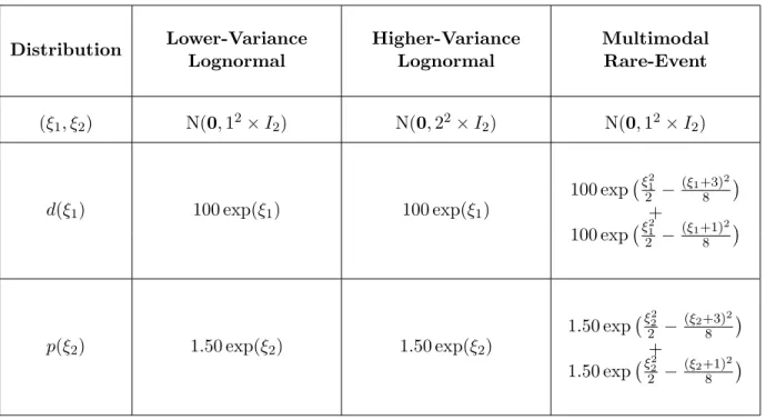
In our numerical experiments, we investigate the sampling properties of MCMC-IS by pairing this model with three separate distributions: a lower-variance lognormal distribution, a higher-variance lognormal distribution, and a multimodal rare-event distribution. The parameters used to generate the demand and sales price for these distributions are specified in Table 4.1.
4.1.2 A Multidimensional Extension
The D-dimensional Newsvendor model is a multidimensional extension of the Newsven-dor model specified in Section 4.1.1. In this extension, we consider a problem where the
Distribution Lower-Variance Lognormal Higher-Variance Lognormal Multimodal Rare-Event (ξ1, ξ2) N(0,12×I2) N(0,22×I2) N(0,12×I2) d(ξ1) 100 exp(ξ1) 100 exp(ξ1) 100 exp ξ21 2 − (ξ1+3)2 8 + 100 exp ξ21 2 − (ξ1+1)2 8 p(ξ2) 1.50 exp(ξ2) 1.50 exp(ξ2) 1.50 exp ξ22 2 − (ξ2+3)2 8 + 1.50 exp ξ22 2 − (ξ2+1)2 8
Table 4.1: Parameters of demand and sales price distributions for the Newsvendor model.
Newsvendor has to sell D2 different types of newspapers which have the same demand and sales price distribution. The recourse function of theD-dimensional Newsvendor model can be expressed as, QD(xb) = D 2 X i=1 Qi(xbi) (4.3)
where Qi(bxi) denotes the 2-dimensional recourse function used to represent the expected
future costs associated with a single type of newspaper as in (4.2).
4.1.3 A Multistage Extension
TheT-stage Newsvendor model is a multistage extension of the Newsvendor model specified in Section 4.1.1. In this extension, we consider a problem where the Newsvendor buys and sells a single type of newspapers over T consecutive days. We assume that any newspapers that are to be sold on day t+ 1 have to be bought on dayt, and that any unsold newspapers at the end of day t + 1 have to be recycled at a price of r. These assumptions allow us to extrapolate the true values of optimal solution x* and optimal cost z* for a T-stage Newsvendor model from their corresponding values for the Newsvendor model specified in Section 4.1.1. In particular, we reason that the optimal cost z* scales additively with the
number of time periods, and the optimal solution x* remains the same.
4.2
Experimental Setup
4.2.1 Experimental Statistics
The advantages of using the two-stage, two-dimensional Newsvendor model in Section 4.1.1 are that the relevant distributions can be easily visualized, and that we can determine the true value of the recourse function at different values of bx using state-of-the-art numerical integration procedures. In turn, we can also determine the true values of the recourse function for the multidimensional and multistage extensions of the Newsvendor problem that are specified in Sections 4.1.2 and 4.1.3.
By knowing the true values of the recourse function for these SP models, we can con-sider both the error and the variance of the estimates that are produced in our numerical experiments. Table 4.2 provides an overview of the different statistics that we report in Sections 4.3 - 4.8. We note that the statistics in these sections have been generated using
R= 100 repetitions, and have been normalized for clarity. We note that that all the results for the MCMC-IS method have been generated using Mγ +N functional evaluations as we explain further in Section 4.5, whereγ denotes the acceptance rate of the MCMC algorithm in MCMC-IS.
4.2.2 Implementation
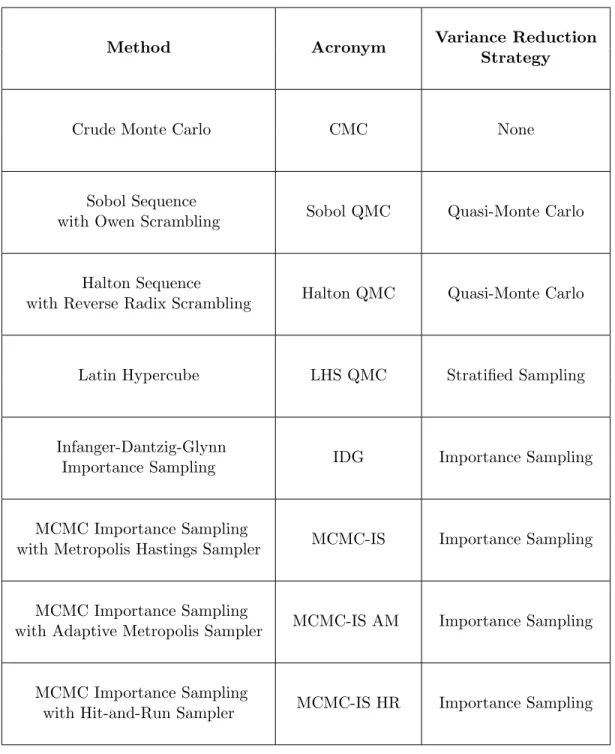
Table 4.3 summarizes the different sampling methods that refer to in Sections 4.3 - 4.5. Unless otherwise stated, we produced all results for these methods in MATLAB 2012a. In particular, we used a built-in Mersenne-Twister algorithm to generate the uniform random numbers for the CMC, LHS, IDG and MCMC-IS sampling methods. Similarly, we used built-in Owen and Reverse-Radix scrambling algorithm to randomize the sequences that we generated for Sobol QMC and Halton QMC methods. Most of the results for MCMC-IS were generated using the simple implementation described in Section 3.3. We built all approximate importance sampling distributions for MCMC-IS using the MATLAB KDE Toolbox, which is available online at http://www.ics.uci.edu/~ihler/code/kde.html.
Statistic Formula Description MSE(Qb) v u u t1 R R X i=1 (Q(xb)−Qb(bx)i)2 mean-squared error ofR
estimates of the value of the recourse function Qb atbx SE(Qb) 1 R R X i=1 1 N 1 N −1 v u u tQb(bx)i− 1 N N X j=1 Q(bx, ξj) 2 mean ofR estimates of
standard error in the value of the recourse functionQb atbx
MSE(bg) R1 R X i=1 1 N p (g(ξi)−bg(ξi))2 mean-squared error ofR approximations of the zero-variance distributions at b
x; theξis are specified by a
100×100 grid on Ξ
Table 4.2: Sampling statistics reported in Chapter 4.
4.3
Sampling from the Important Regions
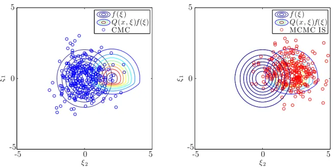
Importance sampling is most effective when an importance sampling distribution can gener-ate samples from regions that contribute the most to the value of the the recourse function. Such regions are referred to as the important regions of the recourse function, and occur at points where |Q(bx, ξ)|f(ξ) attains large values. Accordingly, the major difference between MCMC-IS and other MC methods is that MCMC-IS generates samples at important areas of the recourse function using the importance sampling distribution bgM.
We illustrate this difference by plotting the location of the samples that are used to esti-mate the recourse functionQ(xb) atbx = 50 for a Newsvendor model assuming a lower-variance lognormal distribution in Figure 4-1, and Newsvendor model paired with a a multimodal rare-event distribution in Figure 4-2.
As shown in Figures 4-1 and 4-2, the samples that are generated using the MCMC-IS importance sampling distribution bgM are located at important regions of the recourse function, where |Q(bx, ξ)|f(ξ) attains high values. In contrast, the samples generated using