No. 2007/25
Capturing Common Components in
High-Frequency Financial Time Series: A Multivariate
Stochastic Multiplicative Error Model
Center for Financial Studies
The
Center for Financial Studies
is a nonprofit research organization, supported by an
association of more than 120 banks, insurance companies, industrial corporations and
public institutions. Established in 1968 and closely affiliated with the University of
Frankfurt, it provides a strong link between the financial community and academia.
The CFS Working Paper Series presents the result of scientific research on selected
topics in the field of money, banking and finance. The authors were either participants
in the Center´s Research Fellow Program or members of one of the Center´s Research
Projects.
If you would like to know more about the
Center for Financial Studies
, please let us
know of your interest.
* Acknowledgements: Earlier versions of this paper have been presented at the EC2 conference 2003 in London, at the International Conference on Finance in Copenhagen, 2005, the 2005 Arne Ryde Workshop in Financial Economics in Lund, the International Conference on High Frequency Finance in Konstanz, 2006, the 2006 meeting of the European Econometric Society in Vienna as well as the 2006 meeting of the German Economic Association in Bayreuth. For valuable comments we would like to thank Torben G. Andersen, Luc Bauwens, Tim Bollerslev, Robert F. Engle, Timo Ter¨asvirta, Winfried Pohlmeier as well as the seminar participants at the Stockholm School of Economics and the Universit´e Libre de Bruxelles.
1 Institute for Statistics and Econometrics, School of Business and Economics as well as Center for Applied Statistics and Economics
CFS Working Paper No. 2007/25
Capturing Common Components in High-
Frequency Financial Time Series: A Multivariate
Stochastic Multiplicative Error Model *
Nikolaus Hautsch
1July 2007
Abstract:
We introduce a multivariate multiplicative error model which is driven by
componentspecific observation driven dynamics as well as a common latent
autoregressive factor. The model is designed to explicitly account for (information driven)
common factor dynamics as well as idiosyncratic effects in the processes of
high-frequency return volatilities, trade sizes and trading intensities. The model is estimated by
simulated maximum likelihood using efficient importance sampling. Analyzing five
minutes data from four liquid stocks traded at the New York Stock Exchange, we find that
volatilities, volumes and intensities are driven by idiosyncratic dynamics as well as a
highly persistent common factor capturing most causal relations and cross-dependencies
between the individual variables. This confirms economic theory and suggests more
parsimonious specifications of high-dimensional trading processes. It turns out that
common shocks affect the return volatility and the trading volume rather than the trading
intensity.
JEL Classification:
C15, C32, C52
Keywords:
Multiplicative Error Models, Common Factor, Efficient Importance Sampling,
Intraday Trading Process
1
Introduction
Numerous empirical studies have documented a strong positive contemporaneous relation
between daily aggregated volume and volatility. This observation is consistent with the
mixture‐of‐distribution hypothesis (MDH) pioneered by Clark (1973). The MDH relies on
”large” amount of intradaily logarithmic price changes associated with ”pseudo” intraday equilibria. The assumption that these intraday price changes are also accompanied by an increased trading volume leads to an extension of Clark’s model and implies a positive contemporaneous correlation between daily volume and volatility.1
Whereas the employed central limit arguments provide a sensible framework for aggre-gated (daily) data, they are not applicable on a high-frequency level since the number of underlying ”pseudo” equilibria cannot be large but converge to zero when we approach the transaction level. Nevertheless, under the assumption that daily volumes and returns, both consisting of intraday aggregates, are driven by a subordinated common process, then the latter should be identifiable also on an intraday level. Actually, the idea of an underlying (unobservable) information process is also consistent with most asymmetric information based market microstructure models as e.g. introduced by Glosten and Milgrom (1985) and Easley and O‘Hara (1992). In these settings, positive contemporaneous correlations between trading volumes and volatilities arise by the interaction among asymmetrically in-formed market participants. However, market microstructure theory is typically relatively vague, if not silent, regarding the underlying time horizon and thus the frequency on which common information-induced effects should be observable. On the other hand, several em-pirical studies provide evidence for common movements and strong interdependencies in high-frequency volatilities and trading intensities2 supporting the notion of an underlying common component jointly driving trading activity and volatility.
In this study, we aim to analyze whether a common component in volatilities and trading volumes is identifiable not only based on daily data but also on higher sampling frequencies, such as e.g. five minutes. We associate this hypothesis with a ”micro-foundation” of the volume-volatility relationship. In this context, we will answer the following research ques-tions: (i) To which extend do the interdependencies between volume and volatility reflect (”true”) causal relationships or rather spurious correlations due to the subordination to the same latent (information arrival) process? (ii) Are potential common movements with volatilities rather reflected in trade sizes or trading intensities or both? (iii) Which of the particular components of the trading process react strongest to a common (information) shock? (iv) How strong and important are remaining serial interdependencies between the individual components even when a common dynamic factor is explicitly taken into ac-count? (v) Does the inclusion of a common latent component leads to more parsimonious specifications of high-dimensional trading processes?
1 See Epps and Epps (1976), Tauchen and Pitts (1983), Lamoureux and Lastrapes (1990), Andersen
(1996) or Liesenfeld (2001).
2See e.g. Engle (2000), Grammig and Wellner (2002), Renault and Werker (2003), Manganelli (2005),
To address these questions, we propose modelling the return volatility, the averaged trade size, and the number of trades per time in terms of a new type of multiplicative error model (MEM) which is driven by two different dynamic processes: a common autoregressive latent factor with component-specific sensitivity and an observation driven (VARMA type) dynamic capturing idiosyncratic effects. The resulting model is calledstochastic multiplica-tive error model (SMEM) and extends the multiplicative error structures as suggested by Engle (2002) and Manganelli (2005) by a latent factor dynamic.
The proposed approach is motivated by two major aspects: Firstly, a well known result in the literature on tests of the MDH is that a single latent component is typically not suffi-cient to fully capture the short-run dynamic dependencies in both volume and volatility. As argued e.g. in Andersen (1996) and Bollerslev and Jubinski (1999), it is likely that different types of ”news”, such as scheduled macroeconomic announcements, option expiration days or company specific earnings announcements affect the volatility and volume processes dif-ferently. For instance, macroeconomic announcements lead to relatively short-lived jumps in volatility but to longer-lasting increases of the trading volume. In contrast, earnings announcements are typically accompanied by strong price shifts combined with relatively little trading activity. Including such idiosyncratic effects requires to account for additional factors. However, instead of allowing for multiple latent factors (as e.g. in Liesenfeld, 2001), the SMEM captures these effects in terms of observation driven dynamics. This idea has been suggested by Bauwens and Hautsch (2006) and leads to a still flexible, but computa-tionally less burdensome specification since only one factor is assumed to be unobservable and has to be integrated out.
Secondly, combining a common latent dynamic with (multivariate) observation driven components can be seen as a reduced form description of the trading dynamics generated by a subordinated information process and by asymmetrically informed market agents. In asymmetric information based market microstructure models3, (uninformed) traders try to infer the existence of information by observing the recent trading history. This leads to distinct (cross-)autocorrelation structures between price changes, volumes, trading in-tensities as well as bid-ask spreads which are tested in a wide range of empirical market microstructure studies.4 In the SMEM, the latent factor can be interpreted as a proxy for the underlying information process which simultaneously affects volatilities, trade sizes and trading intensities. Then, the observation driven dynamics capture component-specific adjustment processes after (possibly information caused) innovation shocks in the
partic-3See, e.g., Glosten and Milgrom (1985), Admati and Pfleiderer (1988), Easley and O‘Hara (1992), Blume,
Easley, and O‘Hara (1994) and Easley, Kiefer, O‘Hara, and Paperman (1996) among others.
4See e.g. Engle (2000) and Manganelli (2005) or the surveys by Bauwens and Giot (2001) or Hautsch
ular trading variables. The latter effects reflect how common information is processed in the market and how market participants’ conditional expectations on future volatilities and trading volumes are updated based on theobservable trade history.
Though the SMEM cannot be seen as a structural model, it nevertheless allows us to study trading processes in a more structural way than in completely reduced form descrip-tions of trading processes (as e.g. Hasbrouck, 1991 Dufour and Engle, 2000, Engle, 2000 or Manganelli, 2005). Disentangling the trading dynamics in the proposed form makes it possible to explicitly control for a common factor and therefore enables us to analyze to which extend the individual trading components reflect (unobservable) joint information. For instance, based on daily data, Jones, Kaul, and Lipson (1994) show that the positive relation between volatility and average trade size is statistically insignificant when the ef-fects of the number of transactions on stock return volatility are taken into account. In contrast, Xu and Wu (1999), Chan and Fong (2000) and Huang and Masulis (2003) find that the average trade size contains nontrivial information for return volatility. Tran (2006) decomposes the return volatility into an erratic factor (being particularly sensitive to new information) as well as a persistent factor and shows that both the trading intensity and
the average trade size are positively correlated with the former. Our study contributes to this literature and sheds some light on the specific information content of the individual trading components.
The SMEM is estimated by simulated maximum likelihood (SML). The computation of the likelihood requires to integrate the latent component out leading to an integral of the dimension of the sample range. To approximate the likelihood function numerically we suggest using the efficient importance sampling (EIS) algorithm proposed by Richard (1998) and Richard and Zhang (2005). In the empirical applications, it turns out that the SML-EIS estimation of the SMEM works very efficiently and is computationally feasible.
In the empirical analysis, we use five minutes aggregates from four highly liquid stocks traded at the New York Stock Exchange (NYSE). Strong empirical evidence for the exis-tence of an autoregressive common component is provided. We find that the unobservable factor is a major driving force of the interdependencies as well as the contemporaneous relations between the individual trading components. Hence, most causal effects between volatility, trade size and trading intensity are indeed driven by a common factor confirming the notion of an underlying information process. It turns out that the latent component has a particularly strong effect on the return volatility as well as the average trade size which confirms the findings based on daily data (see e.g. Tauchen and Pitts, 1983, Chan and Fong, 2000 or Liesenfeld, 2001) and can be seen as a ”micro-foundation” of the daily volume-volatility relationship. In contrast, the trading intensity is only weakly affected
by the underlying component which is contrast to the results by Jones, Kaul, and Lipson (1994). Moreover, it is shown that the inclusion of the latent component clearly improves the goodness-of-fit as well as the dynamical and distributional properties of the model. This illustrates the usefulness of combining observation driven and parameter driven dynamics and opens up new directions to estimate and predict trading processes.
The remainder of the paper is organized in the following way: Section 2 presents the SMEM while Section 3 discusses its statistical properties. In Section 4, we illustrate the statistical inference. Section 5 shows the data and discusses the estimation results. Finally, Section 6 concludes.
2
The Multivariate Stochastic Multiplicative Error Model
Define {Yi, Vi, ρi}, i = 1, . . . , N, as the three-dimensional time series associated with the
intraday process of returns, transaction volumes and trading intensities, respectively. In particular,Yi corresponds to the log return measured over equi-distant time intervals (here
five minutes intervals), Vi is the average volume per trade in the i-th interval and ρi is
the number of trades occurring during interval i. Furthermore, λi is defined as a
com-mon unobservable component that simultaneously influences Yi, Vi and ρi and follows an
autoregressive process which is updated in every interval i.
DefineWi ={wj}ij=1 withwi = (Yi, Vi, ρi)′ and Λi={λj}ij=1 and denoteFi := (Wi,Λi)
as the history of the process up to period i. Following Engle (2000) and Manganelli (2005), we propose decomposing the joint conditional density givenFi−1,f(Yi, Vi, ρi, λi|Fi−1), into
the product of the corresponding conditional densities. Hence,
f(Yi, Vi, ρi, λi|Fi−1) =f(Yi|Vi, ρi, λi;Fi−1)·f(Vi, ρi, λi;Fi−1) (1)
=f(Yi|Vi, ρi, λi;Fi−1)·f(Vi|ρi, λi;Fi−1)·f(ρi|λi;Fi−1)·f(λi; Λi−1),
where it is assumed thatλidepends only on its own history Λi−1. The chosen decomposition
implies thatVi is weakly exogenous for Yi, whereas ρi is weakly exogenous for both Yi and
Vi. Finally, ρi itself is assumed not to be affected by any contemporaneous variable. Of
course, the order of the variables in the decomposition is somewhat arbitrary and depends on the research objective. Here, we proceed along the lines of Engle (2000) and Manganelli (2005) who are particularly interested in the volatility process given the contemporaneous volume and the contemporaneous trading intensity.
The basic idea of the SMEM is to combineobservation drivendynamics withparameter driven dynamics in a multivariate multiplicative error framework as introduced by Engle (2002) and put forward by Engle and Gallo (2006) and Cipollini, Engle, and Gallo (2007). Then, a three-dimensional SMEM for volatilities, trade sizes and trading intensities is given
by Yi = E[Yi|Fi−1] +ξi, (2) ξi = q hieδ1λish,iηi, ηi∼i.i.d.N(0,1), (3) Vi = Φieδ2λisV,iui, ui∼i.i.d.GG(p2, m2), (4) ρi = Ψieδ3λisρ,iεi, εi∼i.i.d.GG(p3, m3), (5)
where hi, Φi and Ψi denote observation driven dynamic components, ηi, ui and εi are
process-specific innovation terms which are assumed to be independent, andsh,i, sV,i, sρ,i >
0 capture deterministic time-of-day effects in volatilities, trade sizes, and trading intensities, respectively. We assume that the volatility innovationsηifollow a standard normal
distribu-tion whereas the volume and trading intensity innovadistribu-tions ui andεi follow a standard
gen-eralized gamma distribution depending on the parameters p2, m2 and p3, m3, respectively.
The generalized gamma distribution allows for a high distributional flexibility including the cases of over-dispersion and under-dispersion as well as non-monotonic hazard shapes.5
The componenthieδ1λish,i corresponds to the conditional variance of the returns given
Fi−1, λi, and the time of the day. Accordingly, up to a constant multiplicative factor6,
Φieδ2λisV,i and Ψieδ3λisρ,i correspond to the conditionally expected volume and the
condi-tionally expected trading intensity givenFi−1,λi, and the time of the day. Hence, the major
idea of the SMEM is to model these conditional moments on the basis of a multiplicative interaction of the processes{hish,i,ΦisV,i,Ψisρ,i}and eλi. Then, the parametersδ1,δ2 and
δ3 drive the process-specific impact ofλi.
The common latent factorλi is assumed to follow a zero mean AR(1) process, given by
λi =aλi−1+νi, νi ∼i.i.d.N(0,1), (6)
whereνi is assumed to be independent ofηi,uiand εi. Then, the process-specific impact of
the latent factor is given by λij :=δjλi withλij =aλi−1,j+δjνi, and thus dλdνiji >(<) 0 for
δj >(<) 0 withj= 1,2,3. 7 Because of the symmetry of the distribution ofνi, the sign of
the individual parameters δj are not identified. Hence, for instance, we cannot distinguish
between the cases δ1 > 0, δ2 < 0 versus δ1 < 0, δ2 > 0. Nevertheless, we can identify
whether the latent component influences the two components in the same direction or in opposite directions. For that reason, we have to impose an identification assumption which restricts the sign of one of the parameters δj. Then, the signs of all other coefficients δk
with k6=j are identified.
5We refer the specifications presented above explicitly to the processesξi,Viandρi. However, generally,
the proposed structure can be used for any kind of positive-valued random variable including e.g. bid-ask spreads or market depths.
6Note that the means ofui andεiare unequal to one as long as m
2, m3, p2, p36= 1. 7Hence, in order to identify theδj’s, the latent variance Var[νi] is normalized to one.
The process-specific components hi, Φi and Ψi are assumed to follow a multivariate
observation driven dynamic which is parameterized in terms of a VAR(MA) structure
µi =ω+A0z0,i+ P X j=1 Ajzi−j+ Q X j=1 Bjµi−j, (7) where µi:= (lnhi, ln Φi, ln Ψi)′, (8) z0,i:= (0, lnVi, lnρi)′, (9) zi:= | ξi| p hish,i , Vi ΦisV,i , ρi Ψisρ,i !′ =|ηi|eδ1λi/2, uieδ2λi, εieδ3λi ′ (10) as well as ω = {ωk}, k = 1,2,3, denote (3×1) vectors, and A0 = {αkl0 } for k, l = 1,2,3
is a (3×3) triangular matrix where only the three upper right elements can be nonzero. Furthermore, Aj ={αklj } and Bj = {βjkl} for k, l = 1,2,3 are (3×3) matrices of
innova-tion and persistence parameters, respectively. The triangular structure of A0 reflects the
imposed weak exogeneity assumptions underlying the decomposition of the joint density in (1). The log-linear form ensures the positiveness of the individual processes without im-posing additional parameter restrictions. This property eases the estimation of the model particularly when A0 6= 0 or when additional explanatory variables are included.
According to eq. (10) the process-specific dynamics in (7) are updated based on innova-tions zi corresponding to the lagged (de-meaned) returns, volumes and trading intensities,
standardized by their corresponding observation driven components. We choose this speci-fication because of four reasons: Firstly, using standardized (de-meaned) absolute returns, volumes and intensities as innovations is quite common in logarithmic multiplicative error specifications and ensures that the stationarity conditions ofµi (givena) only depend onBj.
This form is chosen e.g. in logarithmic autoregressive conditional duration (Log-ACD) mod-els (Bauwens and Giot, 2000, Bauwens, Galli, and Giot, 2003) or in exponential GARCH models (Nelson, 1991).8 Secondly, standardizing only by observation driven components en-sures that the latter can be updated without requiring to integrate the latent factor out. As discussed in Section 4, this clearly eases the estimation of the model since the computation ofµidoes not depend onλi. Thirdly, since the latent variable is not integrated out from the
innovations, it is clear that the latter implicitly still depend onλi (see (10)). Hence, a shock
in the latent factor in period iinfluences {hi, Φi, Ψi}not only in period i, but (throughzi)
also in the following periods which causes (cross-)autocorrelations between the individual processes. Because of this effect, the common component can generate cross-dependencies
8The specification could be easily extended to allow for nonlinear news responses as e.g. discussed in the
context of ACD models by Fernandes and Grammig (2006) or Hautsch (2006) or in the context of GARCH models by Engle and Ng (1993) or Hentschel (1995).
between the observation driven processes hi, Φi and Ψi even when A0 =Aj = 0. This will
be illustrated in more detail in Section 3 and is an important model feature allowing to parsimoniously capture cross-dependencies. Fourth, with this specification, we implicitly assume that conditional expectations of market participants, given the latent factor, are updated based on the observable history in volatilities, volumes and intensities. Conse-quently, the dynamics in µi capture (cross-)autocorrelations between volatilities, volumes
and intensities which are not driven by an underlying (information) component but are rather attributed to specific trading behavior.
In order to illustrate the structure of the model in more detail, assume for simplicity
A0 = 0, P =Q= 1, sh,i =sV,i =sρ,i = 1, and diagonal parameterizations of A1 and B1.
Then, the model is rewritten as
ξi = q ˜ hiηi, ˜hi=hieδ1λi, (11) Vi = ˜Φiui, Φ˜i= Φieδ2λi, (12) ρi = ˜Ψiεi, Ψ˜i= Ψieδ3λi, (13) where ln ˜hi−δ1λi =ω1+α111 | ξi−1| p hi−1 +β111 (ln ˜hi−1−δ1λi−1), (14) ln ˜Φi−δ2λi =ω2+α221 Vi−1 Φi−1 +β221 (ln ˜Φi−1−δ2λi−1), (15) ln ˜Ψi−δ3λi =ω3+α331 Xi−1 Ψi−1 +β133(ln ˜Ψi−1−δ3λi−1). (16)
Hence, it is evident that the latent component λi can be interpreted as an additional
re-gressor which is statically included and is driven by its own dynamics according to (6). The SMEM is an extension of the multiplicative error models of Engle (2002) and Manganelli (2005). Whereas Manganelli (2005) assumes the process-specific innovations to be contemporaneously uncorrelated, Cipollini, Engle, and Gallo (2007) address the problem of specifying multivariate MEM’s taking into account contemporaneous correlations between the individual processes by means of copula-approaches. The multivariate SMEM proposed in this paper can be seen as an alternative which captures contemporaneous correlations by the inclusion of a common latent factor. The usefulness of the combination of observation driven and parameter driven dynamics is also stressed by Blazsek and Escribano (2005) who propose applying the stochastic conditional intensity model by Bauwens and Hautsch (2006) to model the intensity of patent activities of firms. Koopman, Lucas, and Monteiro (2005) introduce an extension of the model and apply it successfully to model credit rating transitions.
We call the first component of the SMEM a stochastic GARCH (SGARCH) model, whereas the second and third component is referred to a stochastic
ACD (SACD) model. These specifications nest several model classes. The SGARCH model encompasses a simple EGARCH specification as well as the stochastic volatility (SV) model proposed by Taylor (1986) and permits both competing models to be tested against each other. In particular, for α111 =β111 = 0, (14) can be rewritten as an SV model, while for
δ1 = 0 it resembles a simple form of the EGARCH model (however without news impact
asymmetries) as introduced by Nelson (1991). Furthermore, for α11
1 6= 0 andβ111= 0 it can
be interpreted as an SV model that is mixed with a further random variable. Accordingly, the SACD model as specified in (15) and (16) nests the SCD model (Bauwens and Veredas, 2004) for α221 = β122 = 0 and α331 = β133 = 0, respectively, the Log-ACD model (Bauwens and Giot, 2000) for δ2 = 0 and δ3 = 0, respectively, and, correspondingly, a mixed SCD
model for α22
1 6= 0,β122= 0 and α331 6= 0, β133= 0, respectively.
In the univariate case, the SMEM corresponds to a two-factor model which might allow to capture dynamics not only in first conditional moments but also in higher order con-ditional moments. In this sense, the SMEM could serve as an interesting alternative to the stochastic volatility duration model by Ghysels, Gouri´eroux, and Jasiak (2004). More detailed comparisons of both approaches are clear issues for further research.
3
Statistical Properties of the Model
The dynamic stability of the SMEM is ensured by the stability of the two underlying dynamic components. The strict stationarity ofλi is guaranteed by|a|<1. In this case, the
innovations of the observation driven dynamics,zi, consist of products of i.i.d. variates and
strictly stationary variables and thus are themselves strictly stationary. Then, the stability of the observation driven VAR(MA) dynamic characterized by (7) to (10) is ensured by the eigenvalues of the characteristic equation implied by Bj,j= 1, . . . , Q, lying inside the unit
circle.
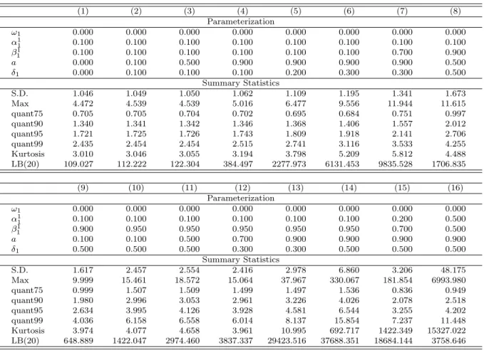
The inclusion of the latent component in the model renders the analytical computation of unconditional moments and (cross-)autocorrelation functions generally relatively diffi-cult. In the following, we analyze the statistical properties of the model based on several simulation studies. For different specifications of the SMEM, we generate 100 sets of 50,000 observations and analyze the distributional and dynamical properties. Tables 1 and 29show the mean, standard deviation, minimum, maximum, kurtosis, selected quantiles as well as the Ljung and Box (1978) statistic for (univariate) SGARCH and SACD processes under dif-ferent parameterizations.10 Table 1 illustrates that the inclusion of a latent component has
9All tables and figures are shown in the Appendix.
10Since the distribution of returns under a SGARCH process is symmetric and the mean is set to zero,
a strong influence on the standard deviation, the kurtosis as well as the serial dependence in the second moments of the simulated return process. We observe that processes generated by high parameter values ofaandδ1 imply a high unconditional variance, overkurtosis, fat
tails as well as a strong serial dependence in the conditional variance. Because of its mixture structure, the SGARCH process allows for a high distributional and dynamical flexibility and captures the well known statistical properties of typical financial return series.
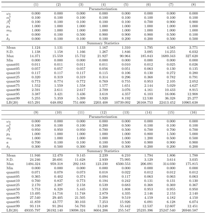
Similar findings are revealed for simulated SACD processes (Table 2). Again, an increase of the latent parameters a and δ3 leads to a significant rise of the unconditional variance
as well as of the autocorrelations of the resulting process. As for SGARCH processes, it is apparent that a high serial dependence in both the observation driven component and the parameter driven component generate distributions with strong fat tail behavior. These effects are even amplified when the Weibull parameter p3 is larger than one.
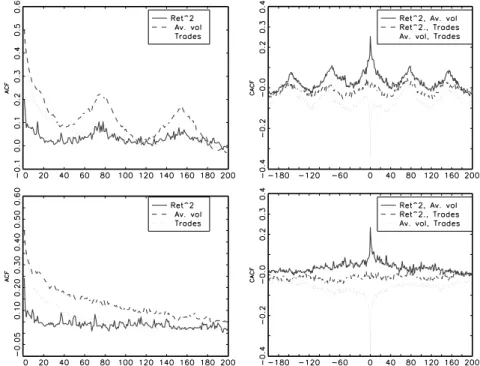
Below we study the dynamic properties of multivariate SMEM’s. Because of brevity we concentrate mainly on the impact of the common latent factor on the dynamic properties of the multivariate process, whereas the influence of the observation driven VARMA com-ponent is of less interest. Figures 1 to 6 show the autocorrelation and cross-autocorrelation functions implied by a two-dimensional SMEM(1,1) for the volatility and the intensity pro-cess.11 Figures 1 to 3 show SMEM processes where the latent factor is strongly (positively) autocorrelated (a = 0.9). Moreover, we impose diagonal specifications of A1 and B1
im-plying no (direct) dependencies between hi and Ψi and assume the autocorrelations of the
processes hi and Ψi to be only quite weak (αii1 = β1ii = 0.1 fori= 1,3). Nevertheless, we
observe that the existence of the latent factor causes distinct autocorrelations inhi and Ψi
as well as inY2
i andρi. As described in Section 2, this is caused by the fact thathi and Ψi
are updated by innovations zi−1 which jointly depend on an autocorrelated common
com-ponent λi−1 (recall eq. (10)). This induces significant serial dependencies in{hi,Ψi, Yi2, ρi}
even for values of A1 and B1 close to zero. Similarly, the latent factor causes also distinct
cross-autocorrelations between both hi and Ψi as well as between Yi2 and ρi even for
di-agonal specifications of A1 and B1. Clearly, the magnitude of the (cross-)autocorrelations
rises with the parameters δ1 and δ3 as well as with the persistence of the latent process as
driven by a. These illustrations show that a persistent latent component can be the major source of the observed cross-dependencies in the multivariate process. This is one of the main features of the model.
Figure 3 shows the effect of the parameters δ1 and δ3 having opposite signs. Since
a, A1 and B1 are unchanged the autocorrelations in {hi,Ψi, Yi2, ρi} are identical to those
11Since the volume component is parameterized similarly, it reveals the same properties and same
inter-actions with the other processes. For this reason, we refrain from showing the results for the corresponding three-dimensional processes.
shown in Figure 2. However, since the latent factor influences the two processes in opposite directions, we observe negative CACF’s between hi and Ψi as well as between Yi2 and
ρi. Hence, it is shown that under certain parameter constellations, the latent factor can
cause positive serial dependencies in Yi2 and ρi while simultaneously inducing negative
cross-autocorrelations between the two processes.
In contrast, Figures 4 and 5 show SMEM processes where the observation driven dynam-ics themselves also reveal distinct cross-dependencies. In Figure 4, λi is set to zero, whereas
in Figure 5, λi follows a persistent process with a = 0.9 and δ1 = δ3 = 0.1. Comparing
both figures demonstrates that the inclusion of the latent factor in Figure 5 induces a sig-nificant rise of the ACF ofhi and Ψi, and of the CACF between Yi2 andρi.12 Hence, if the
latent factor is sufficiently strong, it can completely overlay and dominate the multivariate dynamics. Clearly, the strength of this effect depends on the process-specific impacts d1
and d3.
Finally, Figure 6 illustrates the effects when the latent factor reveals no serial dependence at all (a= 0), however, a strong impact on the individual components (δ1 =δ3 = 1). Then,
the complete process is effectively overlaid by a white noise variable which clearly reduces the persistence in hi, Φi,Yi2 and ρi and drives the cross-autocorrelations toward zero.
Summarizing, we observe that the SMEM is able to capture a wide range of multi-variate dynamics arising either from a common underlying component and/or idiosyncratic observation driven dependencies. Most importantly, it is illustrated that the existence of a persistent common latent factor can be the source of distinct (cross-)autocorrelations and contemporaneous correlations in the multivariate process even when there are no (or weak) multivariate observation driven dynamics. This reflects the idea that an underlying com-ponent can be indeed the major driving force for the observed serial (cross-)dependencies in multivariate trading processes. This will be empirically tested in Section 5.
4
Statistical Inference
LetW denote the data matrix withWi:={wj}ij=1and letθdenote the vector of parameters
of the SMEM. The conditional likelihood given the realizations of the latent variable Λi is
given by L(W;θ|Λn) = n Y i=1 1 p 2˜hiπ exp −ξ 2 i 2˜hi p2Vip2m2−1 Γ(m2) ˜Φpi2m2 exp − Vi ˜ Φi p2 × p3ρ p3m3−1 i Γ(m3) ˜Ψpi3m3 exp − ρi ˜ Ψi p3 , (17)
12The asymmetric cross-autocorrelations betweenY2
i andρiare caused by the fact that the return
where ˜ hi =hieδ1λish,i, ˜ Φi = Φieδ2λisV,i, ˜ Ψi = Ψeδ3λsρ,i.
Since the latent process is not observable, the conditional likelihood function must be integrated with respect to λi using the assumed normal distribution of the latter. Hence,
the integrated log likelihood function is given by
L(W;θ) = Z n Y i=1 1 p 2˜hiπ exp −ξ 2 i 2˜hi p2Vip2m2−1 Γ(m2) ˜Φpi2m2 exp − Vi ˜ Φi p2 × p3ρ p3m3−1 i Γ(m3) ˜Ψpi3m3 exp − ρi ˜ Ψi p3 1 √ 2πexp −12(λi−µ0,i)2 dΛ = Z n Y i=1 g(wi|λi, Wi−1;θ)p(λi|Λi−1;θ)dΛ = Z n Y i=1 f(wi, λi|Wi−1,Λi−1;θ)dΛ, (18)
whereµ0,i:= E[λi|Λi−1],g(·) denotes the conditional density ofwi given (λi, Wi−1) andp(·)
denotes the conditional density of λi given Λi−1. The computation of the n-dimensional
integral in (18) is performed numerically using the efficient importance sampling (EIS) method proposed by Richard and Zhang (2005). This algorithm was shown to work quite well in the context of the class of latent factor models (see e.g. Liesenfeld and Richard, 2003 or, Bauwens and Hautsch, 2006).
To implement the EIS algorithm, the integral (18) is rewritten as
L(W;θ) = Z n Y i=1 f(wi, λi|Wi−1,Λi−1;θ) m(λi|Λi−1, φi) n Y i=1 m(λi|Λi−1, φi)dΛ, (19)
where {m(λi|Λi−1, φi)}ni=1 denotes a sequence of auxiliary importance samplers indexed
by auxiliary parameters φi. Then, the importance sampling estimate of the likelihood is
obtained by L(W;θ)≈LˆR(W;θ) = 1 R R X r=1 n Y i=1 f(wi, λi(r)(φi)|Wi−1,Λ(ir−)1(φi−1);θ) m(λ(ir)(φi)|Λi(−r)1(φi−1), φi) , (20)
where {λ(ir)(φi)}ni=1 denotes a trajectory of random draws from the sequence of auxiliary
importance samplers m andR such trajectories are generated.
The idea of the EIS approach is to choose a sequence of samplers for m(λi|Λi−1, φi)
that exploits the sample information on the λi’s revealed by the observable data. As
shown by Richard and Zhang (2005), the EIS principle is to choose the auxiliary pa-rameters {φi}ni=1 in a way that provides a good match between Πni=1m(λi|Λi−1, φi) and
ˆ
LR(W;θ). Richard and Zhang (2005) illustrate that the resulting high-dimensional
mini-mization problem can be split up into solvable low-dimensional subproblems. This makes the approach tractable even for very high dimensions. The detailed EIS procedure is de-scribed in the appendix.
An important advantage which facilitates the computation of the function f(·) is the fact that the time series recursion of the observation driven components hi, Φi and Ψi can
be computed without the need of knowing the latent factor. As discussed in Section 2 this is due the fact that {hi,Φi,Ψi} are driven based on innovations zi which are observable
given the history of {ξi, Vi, ρi} and {hi,Φi,Ψi}. Then, hi, Φi and Ψi can be computed in
a first step according to the VARMA structure given by (7) to (10) and can be used in a second step to evaluate the sampler {m(λi|Λi−1, φi}ni=1.
Filtered estimates of functions of an arbitrary function ofλi,ϑ(λi), given the observable
information set up to ti−1 are given by
E [ϑ(λi)|Wi−1] = R ϑ(λi)p(λi|Wi−1,Λi−1, θ)f(Wi−1,Λi−1|θ)dΛi R f(Wi−1,Λi−1|θ)dΛi−1 . (21)
The integral in the denominator corresponds to the marginal likelihood function of the first i−1 observations, L(Wi−1;θ), and can be evaluated on the basis of the sequence
of auxiliary samplers {m(λj|Λj−1,φˆji−1)}ij−=11 where {φˆij−1} denotes the value of the EIS
auxiliary parameters associated with the computation ofL(Wi−1;θ) andθis set equal to its
corresponding maximum likelihood estimate. Correspondingly, the numerator is computed by 1 R R X r=1 ϑλ(ir)(θ) i−1 Y j=1 fwj, λ(jr)( ˆφij−1)|Wj−1,Λ(jr−)1( ˆφ i−1 j−1), θ mλ(jr)( ˆφi−1 j )|Λ (r) j−1( ˆφji−−11),φˆij−1 , (22) where {λ(jr)( ˆφi−1
j )}ij−=11 denotes a trajectory drawn from the sequence of importance
sam-plers associated withL(Wi−1;θ), andλ
(r)
i (θ) is a random draw from the conditional density
p(λi|Wi−1, Λi(−r)1( ˆφii−−11), θ). The computation of the sequence of filtered estimates
E [ϑ(λi)|Wi−1], i = 1, . . . , n, requires to rerun the EIS algorithm for every i (=1 to n).
Then, the filtered residuals are given by ˆ ηi= ˆ ξi q ˆ hiE [eδ1λi|Wi−1] ˆsh,i (23) ˆ ui= ˆ Vi ΦiE [eδ2λi|Wi−1] ˆsV,i (24) ˆ εi= ρi ˆ ΨiE [eδ3λi|Wi−1] ˆsρ,i . (25)
5
Empirical Results
5.1 Data and Descriptive Statistics
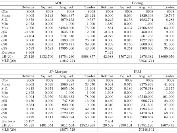
The empirical study uses transaction data from the AOL, Boeing, IBM and JP Morgan stock traded at the New York Stock Exchange (NYSE). The data is extracted from the Trade and Quote (TAQ) database released by the NYSE and covers a period over five months between 02/01/2001 and 31/05/2001.
We choose an aggregation level of five minutes as a trade-off between utilizing a max-imum amount of intraday information on the one hand, ending up with tractable sample sizes on the other hand and, in addition, reducing the influence of too much noise induced by market microstructure effects (like effects due to price-discreteness, split-transactions, liquidity induced price impacts or the irregular spacing in time). Consequently, the re-sulting time series consist of 8,008 observations of five minutes log midquote returns, the average five minutes trading volume per transaction and the number of trades occurring in each interval. Table 3 shows the mean, standard deviation, minimum, maximum, different quantiles, kurtosis as well as univariate and multivariate Ljung-Box statistics associated with the individual time series. The latter is computed according to Hosking (1980) and is given by M LB(s) :=n(n+ 2) s X j=1 1 n−jtrace ˆ C′ jCˆ0−1CˆjCˆ0−1 ∼ χ2ks,
wherek= 3 denotes the dimension of the process,sthe number of lags taken into account, and ˆCj is the jth residual autocovariance matrix.13 The quite high Ljung-Box statistics in
Table 3 indicate that the five minutes trading data reveal strong serial (cross-)dependencies. Since we are not particularly interested in the conditional mean function of returns, we reduce the complexity of the model by estimatingξi in a separate step as the residuals of an
ARMA(1,1) process for theYi series.14 In a next step, we estimate the intraday seasonality
componentssh,i, sV,i, sρ,i. A simultaneous estimation of seasonality effects in the SMEM is
theoretically possible, however, considerably increases the computational burden because of the high number of parameters. For this reason, we exploit the multiplicative structure in (3)-(5) and estimatesh,i, sV,i, sρ,i in a separate step on the basis of cubic spline functions
using 30 minutes nodes.15 Finally, we use ξi/
p
ˆ
sh,i, Vi/sˆV,i and ρi/ˆsρ,i to estimate the
SMEM.16
13Fork= 1, the multivariate Ljung-Box statistic reduces to the well known univariate one.
14However, since for all return series the ARMA component is very close to zero, and thusξiis very similar
toYi, we refrain from showing the estimates here.
15The componentsh,iis estimated based on squared log returns.
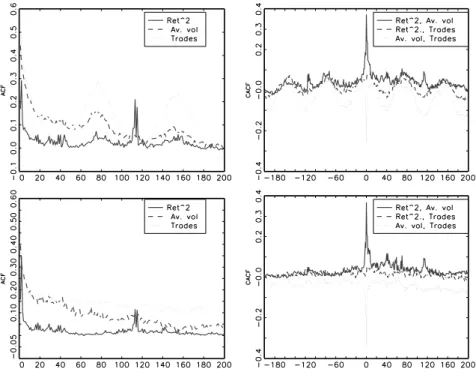
Figures 7 through 10 show the empirical autocorrelation and cross-autocorrelation func-tions of Yi2, Vi, and ρi as well as Yi2/sˆh,i, Vi/sˆV,i, and ρi/sˆρ,i. It turns out that all
pro-cesses reveal significantly positive autocorrelations with a relatively high persistence. The highest serial dependence is observed for volumes and trading intensities, whereas for the volatility process lower autocorrelations are found. Moreover, significantly positive cross-autocorrelations between the return volatility and the trading volume are observed whereas the interdependencies between the volatility and the trading intensity are only very weak. In contrast, significantly negative cross-autocorrelations between the trading volume and the trading intensity are found. Hence, obviously, higher volumes enter the market with a lower speed.
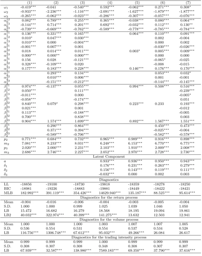
5.2 Estimation Results for Univariate SMEM’s
Tables 4 to 6 show the estimation results of univariate SGARCH as well as SACD models for five minutes volatilities, trading volumes and trading intensities for the four stocks. To restrict the computational effort, we restrict the class of considered models to specifications with a maximal lag order of two. For all processes and all stocks, we find significant evidence for the existence of a persistent latent component. As revealed by the estimates of the parameter a, the strongest serial dependence in the latent component is observed for the volatility and trading intensity processes, whereas it is lower for trading volumes. It turns out that both the parameter driven dynamic as well as the observation driven dynamic interact. In particular,adeclines when observation driven dynamics are included. Accordingly, in the observation driven component, the innovation parameter declines and the persistence parameter is driven toward one when the latent factor is taken into account. Hence, news enter the model primarily through the latent component, which is in line with the idea that the underlying factor serves as a proxy for the unobserved information process. Furthermore, it is shown that the inclusion of the latent component increases the goodness-of-fit as well as the dynamical properties of the model. Actually, for the volatility and the volume processes, a pure parameter driven dynamic in form of a SV or SCD specification, respectively (column (3)), outperforms a pure observation driven dynamic in form of an EGARCH or Log-ACD specification, respectively (column (2)). Nevertheless, we observe that neither the parameter driven component nor the observation driven component can be rejected. Hence, for nearly all time series, the best goodness-of-fit is obtained by specifications (4) or (5) which include bothtypes of dynamics. This result illustrates that the dynamics in volatilities, volumes and trading intensities are not sufficiently captured by a one-factor model but rather by a two-factor model. This observation is in line with the
in intraday trading variables. For reasons of brevity we do not include them in the paper but they are available upon request from the author.
findings by Ghysels, Gouri´eroux, and Jasiak (2004) on the basis of a stochastic volatility duration model.
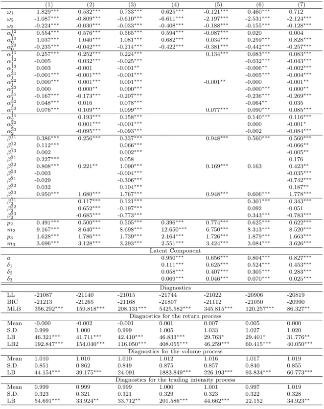
5.3 Estimation Results for Multivariate SMEM’s
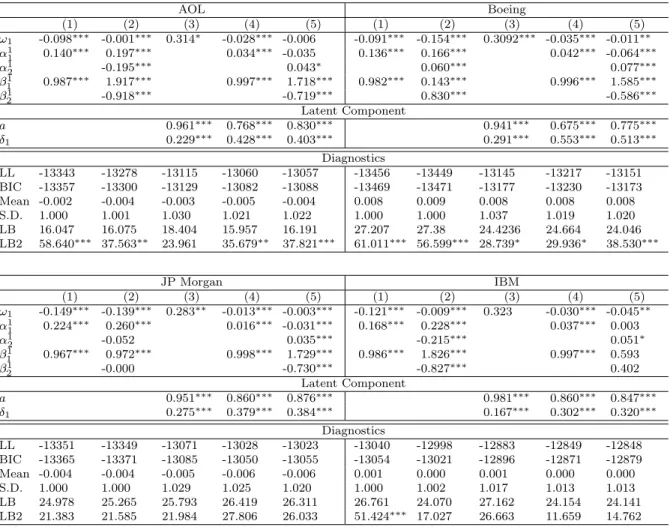
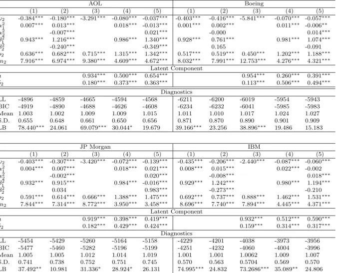
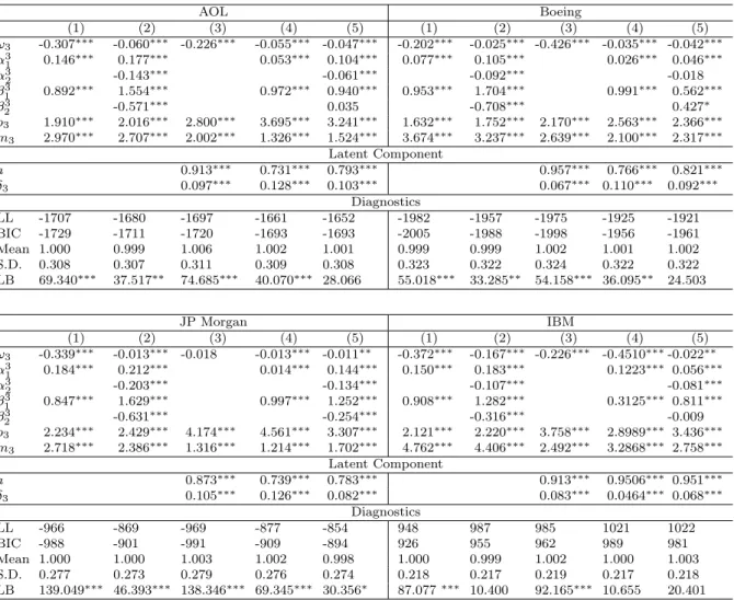
Tables 7 to 10 give the estimation results for multivariate SMEM’s including all three trading components. In order to identify the sign of the parameters δj, we restrict δ1 to
be positive. As in the univariate models, we ensure model parsimony by restricting the maximal lag order to two. In addition, we restrictA2 andB2 to be diagonal matrices. The
major findings can be summarized as following:
(i) We find significant evidence for the existence of a latent common component with an autoregressive parameter which is on average around ˆa≈0.94. Hence, common shocks are relatively persistent over time which is in accordance with corresponding results based on daily data (see e.g. Bollerslev and Jubinski, 1999). Obviously, the latent factor seems to capture common long-run dependence which is not easily covered even by highly parame-terized observation driven dynamics. This result is surprisingly robust over all individual specifications and is clearly in line with the notion of a joint underlying information process. Hence, our results provide evidence that such a process is identifiable not only based on daily data but also based on intraday data.
(ii) The estimated parameters δ1, δ2 and δ3 are significantly positive indicating that
a latent shock affects the volatility, the average trading volume and the trading intensity in the same direction. Interestingly, it turns out that the underlying joint component influences primarily the volatility and trade size, whereas its impact on the trading intensity is comparably weak.17 This finding illustrates that the common factor mainly drives the
well-known volatility-volume relation confirming the corresponding findings for daily data. It also shows that volatility is primarily correlated with the average trade size rather than with the trading intensity. Hence, in contrast to the findings by Jones, Kaul, and Lipson (1994) we find that (unobserved) information is obviously stronger reflected in the average trade size rather than in the trading intensity. Consequently, the former should be a more reliable proxy for the existence of information than the latter.
(iii) The inclusion of the latent factor leads to a significant decline of the magnitude of the parameters α120 and α130 . This indicates that theconditional contemporaneous correlations between ξi2 and Vi as well as between ξi2 and ρi given λi are lower than the corresponding
unconditional correlations. Hence, a significant fraction of the contemporaneous relations between the conditional return variance and the average trade size as well as the trading intensity actually do arise because of the existence of a common component. Nevertheless,
the fact that the joint factor does not fully explain the contemporaneous dependencies indicates that there exist relations between the individual variables which are not necessarily linked to a common information process but rather to trading effects. Actually, the latter might be attributed to the effects that a high liquidity demand associated with high volumes and fast trading leads to significant revisions in the best ask/bid quotes and thus to an increase in (midquote) return volatility.
In contrast, the parameter α230 is significantly negative and widely unaffected by the inclusion of the latent component. Consequently, we can conclude that the (negative) con-temporaneous relation between trade size and trading intensity is not driven by a latent common component. Rather, we identify two opposite effects: Firstly, a positive contem-poraneous correlation between trade size and trading intensity due to the existence of a common subordinated process which affects both processes in the same direction. Secondly, a negative conditional correlation given the latent factor, which is very robust and might be explained by the typical finding that high trading volumes absorb a non-trivial part of the offered liquidity supply. This induces a revision of the best bid/ask quote which makes trading more expensive and thus reduces traders’ incentive for market order trading (see e.g. Foucault, 1999). Our results indicate that the latter is obviously not linked to a potential underlying information component.
(iv) The estimations omitting a common latent component (panels (1)-(3)) clearly reveal significant evidence for cross-dependencies between the volatilities, volumes and trading intensities. In particular, as indicated by a mostly positive parameter ˆα121 , we observe a positive relation between innovations in the lagged trade size and the current volatility. Hence, higher than expected volumes imply significant quote revisions and consequently increase the subsequent volatility. As revealed by ˆα321 >0, this effect is also accompanied by an increase of the trading intensity. In contrast, unexpected increases of the volatility reduce both the subsequent trade size and the trading intensity (ˆα211 <0 and ˆα311 <0). This result is very much in line with theory (see e.g. Foucault, 1999), where a higher transitory volatility increases the spreads and thus makes trading more expensive which in turn reduces the trade sizes and trading intensity.
However, as shown in panels (5)-(7), the inclusion of λi clearly reduces the magnitude
of the aforementioned cross-effects. In most cases, the latter become close to zero and/or insignificant. Similar effects are also observed for the non-diagonal elements in B1. This
finding indicates that the latent common component indeed captures a substantial part of the cross-dependencies. Hence, most of the observed causalities between the individual variables are mainly due to the existence of a subordinated common (information) process
jointly directing the individual components.18 This suggests the usefulness of more
par-simonious parameterizations of the observation driven dynamics which might be mainly reduced to a diagonal specification of the autoregressive parameter matrices.
Moreover, the inclusion of the latent factor reduces the impact of the own process-specific innovations (ˆαii
1 andαii2 fori= 1,2,3) and increases the persistence in the observation driven
dynamics. Hence, in accordance with the results for the univariate models, we find evidence that news enter the model primarily through the latent factor, whereas the impact of the process-specific innovations declines.
(v) In most cases, the specifications without latent factor (columns (1) to (3)) are not able to completely capture the dynamics of the system as indicated by highly significant Ljung-Box statistics for the residuals. Typically, the inclusion of the latent component improves the dynamic properties of the model. This is particularly true for the volatility and the volume component, whereas in some cases the dynamics in the trading intensity are still not completely captured by the model. The latter results are not surprising given that the latent factor’s impact on the trading intensity is only very weak. Moreover, the inclusion of the latent factor leads to a reduction of the multivariate Ljung-Box statistic indicating that the latent component does a good job in capturing the multivariate dynamics and interdependencies between the individual processes. Furthermore, as revealed by the Bayes information criterion (BIC), the SMEM yields a clearly better goodness-of-fit compared to MEM’s without a latent factor.
(vi) The worst performance is observed for specification (4), where any observation driven dynamics are omitted and only a parameter driven dynamic is included. Hence, a single common autoregressive component is not sufficient to completely capture the dy-namics of the multivariate system which is in line with the findings by Andersen (1996) or Liesenfeld (1998). Therefore, as in the univariate models we can neither reject the parame-ter driven dynamic nor the observation driven dynamic. Actually, the best performance is revealed by specifications which include both types of dynamics confirming the basic idea of the proposed model.
Our results are widely robust over the cross-section of stocks. A notable exception are the findings for the Boeing stock which deviate in several respects from those for the other stocks. Here, the latent factor is clearly less persistent and does not capture the dynamics of the processes very well.
18A notable exception is the negative relation between past innovations in the volatility and the current
average trade size as reflected by ˆα21<0. This relationship is obviously not information-driven and becomes even more pronounced when the latent factor is taken into account. This finding is not easily explained in the given setting and requires further investigations.
5.4 Impulse Response Dynamics and Graphical Illustrations
In order to analyze the impact of shocks on the SME process, we rely on the concept of the generalized impulse response function (GIRF) introduced by Koop, Pesaran, and Potter (1996) which is given by
GIRFXi(s, δ,Fi−1) = E[Xi+s|̟i =δ,Fi−1]−E[Xi+s|Fi−1], (26) where Xi ∈ {λi, Yi2, Vi, ρi}, ̟i ∈ {νi, ηi, ui, εi}, δ is the magnitude of the shock, and s
denotes the number of periods over which the GIRF is computed. As shown in this rep-resentation, the GIRF conditions on the shock and on the history of the process whereas innovations occurring in intermediate time periods are averaged out. Then, the GIRF can be interpreted as a random variable in terms of the history Fi−1. In nonlinear models,
analytical expressions for the conditional expectations used in (26) are often not avail-able and thus, Monte-Carlo simulation techniques have to be performed. Figures 11 to 14 show the generalized impulse response functions for a shock in the latent innovation νi
with magnitude of one standard deviation. The GIRF is computed by conditioning on the unconditional means E[Xi] and E[̟i] and is estimated by
\
GIRFXi(s, δ,Fi−1) = ˆE [Xi+s|εi= 1,Fi−1]−E [ˆ Xi+s|Fi−1],
where the conditional expectations are estimated by sample averages based on 5,000 sim-ulated paths of Xi, Xi+1, . . . , Xi+h given the corresponding conditioning information and
using the parameter estimates of specification (8) in Tables 7 to 10. For all processes, we ob-serve a positive, persistent response ofξ2
i,Vi andρi due to a shock in the latent component.
In most cases, the impulse response function declines monotonically and approaches zero after around 30-40 lags corresponding to 150-200 minutes. Hence, common (information) shocks remain present in the trading process up to about 3 hours. In accordance with the parameter estimates, these effects are mostly pronounced for the volatility and trade size component but – not surprisingly – only quite weak for the trading intensity.
Figures 15 and 16 show the time series plots of the (filtered) estimates of exp(λi), Yi2,
Vi and ρi for the AOL and IBM stock, respectively.19 It is illustrated that the latent factor
captures common shocks in the volatility and volume component, whereas the intensity component is widely unaffected by co-movements. We observe that there are certain periods, where volatilities, volumes as well as the common factor move in lock-steps, whereas in other periods, the individual processes seem to be clearly disentangled. These results are confirmed by the correlations between the individual components as given by Corr[eλi, ξ2
i] =
19For sake of brevity, the corresponding plots for the two other stocks are not shown, but are available
0.18 (= 0.22), Corr[eλi, v
i] = 0.52 (= 0.55) and Corr[eλi, ρi] =−0.05 (= 0.01) for the AOL
(IBM) stock.20 Hence, we observe significant commonalities between the latent factor and return volatility as well as the trade size but not necessarily with the trading intensity.
6
Conclusions
In this paper, we have proposed a new type of multivariate multiplicative error model for intraday trading processes. The basic idea of the so-called multivariate stochastic multi-plicative error model (SMEM) is to combine a multivariate observation driven (multiplica-tive error) dynamic with an underlying univariate parameter driven factor which jointly affects all individual components of the system. Whereas the observation driven dynamic is updated by process-specific innovations which are completely observable given the pro-cess history, the parameter driven component follows an autoregressive propro-cess which is updated by unobservable innovations independent from the idiosyncratic errors. We pro-pose the model as a tool to identify a common component in multivariate systems while still allowing for idiosyncratic dynamics. It is a computationally more tractable alternative to multiple latent factor models. Moreover, if there is a common component serving as a major source for cross-dependencies between the individual processes, then its explicit con-sideration should result in a more parsimonious specification of the multivariate process. This becomes even more important when the dimension of the process is very high.
The model was designed to allow for the possibility that intraday return volatility, the trade size as well as the trading intensity are driven not only by their own history but also by a joint dynamic latent factor capturing the (unobservable) information process. Apply-ing the model to five minutes data of four blue chip stocks traded at the NYSE leads to the following conclusions: (i) There is significant evidence for the existence of a common unobservable component following persistent dynamics and jointly driving the trading pro-cess. This finding clearly confirms the notion that underlying common dynamics are not only identifiable based on a daily level but also on an intradaily level and thus provides evidence for a ”micro-foundation” of the well-known volume-volatility relationship. (ii) Confirming the results based on daily data (see e.g. Tauchen and Pitts, 1983, or Boller-slev and Jubinski, 1999) the latent factor mostly affects the volatility and trade size but has an only very weak impact on the trading intensity. Consequently, we conclude that the trade size seems to be a more reliable proxy for common information shocks than the trading intensity which is in contrast to the results by Jones, Kaul, and Lipson (1994). (iii) Most causal relations between volatility, trade size and trading intensity are significantly driven by the common component. ”True” causalities not arising from common information
shocks but rather from mechanisms of trading are still identifiable but typically only very weak. (iv) Even under the presence of a common dynamic factor, it is necessary to allow for process-specific dynamics. This suggests that a single latent component is not sufficient to capture the dynamics of the multivariate system and that common (information) shocks are processed in individual ways. (v) In univariate specifications of the individual trading components SMEM’s significantly outperform models without a latent factor. This finding strongly suggests the need for flexible two-factor models and complements the findings by Ghysels, Gouri´eroux, and Jasiak (2004).
The LF-MEM is economically motivated by the idea that trading activity is driven by (i) an underlying information component and (ii) idiosyncratic, process-specific dynamics. This structure can be considered to be a reduced form representation of trading processes arising from asymmetric information based market microstructure theory (see e.g. Easley and O‘Hara, 1992, or Easley, Kiefer, O‘Hara, and Paperman, 1996, among others). The lat-ter assumes that the trading process is driven by the inlat-teractions between informed market participants who can observe the underlying information process and uninformed agents who infer the true value of the traded asset by observing the trading history. Under this assumption, the common parameter driven component serves as a proxy for the unobserved information process whereas the process-specific observation driven dynamics result from the fact that common (observable) shocks are processed in different ways in volatility, trade size and trading intensity.
Our results provide evidence that a substantial part of the cross-dependencies between the individual processes can be captured a common dynamic component. This should open up the possibility to specify high-dimensional trading processes in a more parsimonious way. Future research is devoted to more extensive applications of the model. On the one hand, it might be interesting to analyze the performance of the model when even more dimensions, such as bid-ask spreads or market depths are added. We expect that the importance of the common component in such a setting becomes even stronger. Important applications of such a model will be the prediction of liquidity and trading costs over short intraday time horizons. Here, the expected trading intensity, market depth, bid-ask spread as well as return volatility will be important determinants of expected trading costs and associated risks. The latter are important inputs to generate automated trading-costs-minimizing trading algorithms as more and more heavily used in the financial industry. Moreover, we also plan to confront the model with observable news announcements as an additional component. This should shed some light on the question which obviously missing information is captured by the latent factor and how observable as well as unobservable information interact and jointly drive the trading process. This should lead to a deeper
understanding of how information is processed and how this depends on the state of the market and the institutional environment of the market. Such information might helpful to optimize trading structures as well as corresponding trading models.
References
Admati, A., and P. Pfleiderer (1988): “A Theory of Intraday Patterns: Volume and Price Variability,”Review of Financial Studies, 1, 3–40.
Andersen, T. G. (1996): “Return Volatility and Trading Volume: An Information Flow Interpretation of Stochastic Volatility,”Journal of Finance, 51, 169–204.
Bauwens, L., F. Galli, and P. Giot (2003): “The Moments of Log-ACD Models,” Discussion Paper 2003/11, CORE, Universit´e Catholique de Louvain.
Bauwens, L., and P. Giot (2000): “The Logarithmic ACD Model: An Application to the Bid/Ask Quote Process of two NYSE Stocks,”Annales d’Economie et de Statistique, 60, 117–149.
(2001): Econometric Modelling of Stock Market Intraday Activity. Kluwer Aca-demic Publishers, Boston, Dordrecht, London.
Bauwens, L., andN. Hautsch(2006): “Modelling Financial High Frequency Data Using Point Processes,” Discussion Paper, 2006-80, CORE, Universit´e Catholique de Louvain.
Bauwens, L., and D. Veredas(2004): “The Stochastic Conditional Duration Model: A Latent Factor Model for the Analysis of Financial Durations,”Journal of Econometrics, 119, 381–412.
Blazsek, S., and A. Escribano (2005): “Dynamic Latent Factor Intensity Models of Knowledge Spillovers: Evidence Based on Patent Analysis,” Working Paper Universidad Carlos III de Madrid.
Blume, L., D. Easley, and M. O‘Hara(1994): “Market Statistics and Technical Anal-ysis,”Journal of Finance, 49 (1), 153–181.
Bollerslev, T., and D. Jubinski (1999): “Equity Trading Volume and Volatility: La-tent Information Arrivals and Common Long-Run Dependencies,” Journal of Business & Economic Statistics, 17, 9–21.
Bowsher, C. G. (2006): “Modelling Security Markets in Continuous Time: Intensity based, Multivariate Point Process Models,”Journal of Econometrics, forthcoming.
Chan, K.,andW. Fong(2000): “Trade Size, Order Imbalance, and the Volatility-Volume Relation,”Journal of Financial Economics, 57, 247–273.
Cipollini, F., R. F. Engle, and G. M. Gallo (2007): “Vector Multiplicative Error Models: Representation and Inference,” Mimeo, University of Firenze.
Clark, P. (1973): “A Subordinated Stochastic Process Model with Finite Variance for Speculative Prices,”Econometrica, 41, 135–155.
Dufour, A., and R. F. Engle (2000): “Time and the Impact of a Trade,” Journal of Finance, 55, 2467–2498.
Easley, D., N. M. Kiefer, M. O‘Hara, and J. B. Paperman (1996): “Liquidity, Information and Infrequently Traded Stocks,”Journal of Finance, 4.
Easley, D., and M. O‘Hara(1992): “Time and Process of Security Price Adjustment,”
The Journal of Finance, 47, 577–605.
Engle, R. F. (2000): “The Econometrics of Ultra-High-Frequency Data,” Econometrica, 68, 1, 1–22.
(2002): “New Frontiers for ARCH Models,”Journal of Applied Econometrics, 17, 425–446.
Engle, R. F., and G. M. Gallo (2006): “A Multiple Indicators Model for Volatility Using Intra-Daily Data,”Journal of Econometrics, 131, 3–27.
Engle, R. F., and V. K. Ng (1993): “Measuring and Testing the Impact of News on Volatility,”Journal of Finance, 48, 1749–1778.
Epps, T. W., and M. L. Epps (1976): “The Stochastic Dependence of Security Price Changes and Transaction Volumes: Implications for the Mixture-of-Distributions Hy-pothesis,”Econometrica, 44, 305–321.
Fernandes, M., and J. Grammig (2006): “A Family of Autoregressive Conditional Du-ration Models,”Journal of Econometrics, 130, 1–23.
Foucault, T. (1999): “Order Flow Composition and Trading Costs in a Dynamic Limit Order Market,”Journal of Financial Markets, 2, 99–134.
Ghysels, E., C. Gouri´eroux, and J. Jasiak (2004): “Stochastic Volatility Duration Models,”Journal of Econometrics, 119, 413–433.
Glosten, L. R., andP. R. Milgrom(1985): “Bid, Ask and Transaction Prices in a Spe-cialist Market with Heterogeneously Informed Traders,”Journal of Financial Economics, 14, 71–100.
Grammig, J., andM. Wellner(2002): “Modeling the Interdependence of Volatility and Inter-Transaction Duration Process,”Journal of Econometrics, 106, 369–400.
Hasbrouck, J. (1991): “Measuring the Information Content of Stock Trades,”Journal of Finance, 46, 179–207.
Hautsch, N.(2004): Modelling Irregularly Spaced Financial Data, vol. 539 ofLecture Notes in Economics and Mathematical Systems. Springer, Berlin.
(2006): “Testing the Conditional Mean Function of Autoregressive Conditional Duration Models,” Discussion Paper 2006-06, Finance Research Unit, Department of Economics, University of Copenhagen.
Hentschel, L. (1995): “All in the Family: Nesting Symmetric and Asymmetric GARCH Models,”Journal of Financial Economics, 39, 71–104.
Hosking, J. R. M. (1980): “The Multivariate Portmanteau Statistic,” Journal of the American Statistical Association, 75, 602–608.
Huang, R. D., andR. W. Masulis(2003): “Trading Activity and Stock Price Volatility: Evidence from the London Stock Exchange,”Journal of Empirical Finance, 10, 249–269.
Jones, C. M., G. Kaul, and M. L. Lipson(1994): “Information, Trading, and Volatil-ity,” Journal of Financial Economics, 36, 127–154.
Koop, G., M. H. Pesaran, and S. M. Potter (1996): “Impulse Response Analysis in Nonlinear Multivariate Models,”Journal of Econometrics, 74, 119–174.
Koopman, S. J., A. Lucas, and A. Monteiro(2005): “The Multi-State Latent Factor Intensity Model for Credit Rating Transitions,” Discussion Paper TI2005-071/4, Tinber-gen Institute.
Lamoureux, C. G., and W. D. Lastrapes(1990): “Heteroskedasticity in Stock Return Data: Volume versus GARCH Effects,” Journal of Finance, 45, 221–229.
Liesenfeld, R. (1998): “Dynamic Bivariate Mixture Models: Modeling the Behavior of Prices and Trading Volume,”Journal of Business & Economic Statistics, 16, 101–109.
(2001): “A Generalized Bivariate Mixture Model for Stock Price Volatility and Trading Volume,”Journal of Econometrics, 104, 141–178.
Liesenfeld, R., and J.-F. Richard (2003): “Univariate and Multivariate Stochastic Volatility Models: Estimation and Diagnostics,”Journal of Empirical Finance, 10, 505– 531.
Ljung, G. M., and G. E. P. Box (1978): “On a Measure of Lack of Fit in Time Series Models,”Biometrika, 65, 297–303.
Manganelli, S. (2005): “Duration, Volume and Volatility Impact of Trades,” Journal of Financial Markets, 8, 377–399.
Meddahi, N., E. Renault, and B. Werker (2006): “GARCH and Irregularly Spaced Data,”Economic Letters, 90, 200–204.
Nelson, D. (1991): “Conditional Heteroskedasticity in Asset Returns: A New Approach,”
Journal of Econometrics, 43, 227–251.
Renault, E., andB. J. Werker(2003): “Stochastic Volatility Models with Transaction Risk,” Discussion paper, Tilburg Univeristy.
Richard, J.-F. (1998): “Efficient High-dimensional Monte Carlo Importance Sampling,” Working Paper, University of Pittsburgh.
Richard, J.-F., and W. Zhang (2005): “Efficient High-Dimensional Importance Sam-pling,” Working Paper Pittsburgh University.
Tauchen, G. E., and M. Pitts (1983): “The Price Variability-Volume Relationship on Speculative Markets,” Econometrica, 51, 485–505.
Taylor, S. J. (1986): Modelling Financial Time Series. Wiley, New York.
Tran, D. T. (2006): “Relationship between Persistent and Erratic Volatility Factors and Trading Activity,” Working Paper, Duke University.
Xu, X. E., and C. Wu(1999): “The Intraday Relation between Return Volatility, Trans-actions, and Volume,”International Review of Economics and Finance, 8, 375–397.
Appendix
A Efficient Importance Sampling
To define the importance sampler itself letk(Λi, φi) denote a density kernel form(λi|Λi−1, φi),
given by
where
χ(Λi−1, φi) =
Z
k(Λi, φi)dλi (28)
denotes the integrating constant. The implementation of EIS requires to select a class of density kernels k(·) for the auxiliary samplerm(·) which provide a good approximation to the productf(·)χ(·). As discussed by Richard and Zhang (2005), a convenient and efficient possibility is to use a parametric extension of the direct samplers, Gaussian distributions in this context. Since the function g(·) appearing in (18) is essentially a product of different exponential functions, we propose to approximate it by a normal density kernel
ζ(λi, φ) = exp φ1,iλi+φ2,iλ2i
, (29)
which is itself an exponential function in terms of λi based on the auxiliary parameters
φi = (φ1,i, φ2,i). Exploiting the property that the product of normal densities is itself a
normal density, we parameterize k(·) as
k(Λi, φi) =p(λi|Λi−1;θ)ζ(λi, φi)
and can show that
k(Λi, φi)∝exp (φ1,i+µ0,i)λi+ φ2,i− 1 2 λ2i (30) = exp −2π12 i (λi−µi)2 exp µ2i 2π2 i , where πi2=(1−2φ2,i)−1, (31) µi= (φ1,i+µ0,i)πi2. (32)
Hence, the auxiliary sampler m(·) is a normal distribution with conditional mean µi and
conditional variance π2i. By omitting irrelevant multiplicative factors, we obtain the inte-grating constant as χ(Λi−1, φi) = exp µ2 i 2π2 i − µ2 0,i 2 ! . (33)
As shown by Richard and Zhang (2005), the Monte Carlo variance of ˆLR(W;θ) can be
minimized by splitting the minimization problem intonminimization problems of the form min φi,0, φi R X r=1 n lnfhwi, λ(ir)(θ)|Wi−1,Λ (r) i−1(θ), θ ·χΛ(ir)(θ), φi+1(θ) i −φ0,i−lnk Λ(ir)(θ), φi(θ) o2 , (34)