Patterns With Multiple Satellite Data Sets
Moctar Dembélé1,2 , Markus Hrachowitz2 , Hubert H. G. Savenije2 , Grégoire Mariéthoz1 , and Bettina Schaefli1,3
1Faculty of Geosciences and Environment, Institute of Earth Surface Dynamics, University of Lausanne, Lausanne,
Switzerland,2Faculty of Civil Engineering and Geosciences, Water Resources Section, Delft University of Technology,
Delft, Netherlands,3Now at Institute of Geography (GIUB), University of Bern, Bern, Switzerland
Abstract
Hydrological model calibration combining Earth observations and in situ measurements is a promising solution to overcome the limitations of the traditional streamflow‐only calibration. However, combining multiple data sources in model calibration requires a meaningful integration of the data sets, which should harness their most reliable contents to avoid accumulation of their uncertainties and mislead the parameter estimation procedure. This study analyzes the improvement of model parameter selection by using only the spatial patterns of satellite remote sensing data, thereby ignoring their absolute values. Although satellite products are characterized by uncertainties, their most reliable key feature is the representation of spatial patterns, which is a unique and relevant source of information for distributed hydrological models. We propose a novel multivariate calibration framework exploiting spatial patterns and simultaneously incorporating streamflow and three satellite products (i.e., Global Land Evaporation Amsterdam Model [GLEAM] evaporation, European Space Agency Climate Change Initiative [ESA CCI] soil moisture, and Gravity Recovery and Climate Experiment [GRACE] terrestrial water storage). The Moderate Resolution Imaging Spectroradiometer (MODIS) land surface temperature data set is used for model evaluation. A bias‐insensitive and multicomponent spatial pattern matching metric is developed to formulate a multiobjective function. The proposed multivariate calibration framework is tested with the mesoscale Hydrologic Model (mHM) and applied to the poorly gauged Volta River basin located in a predominantly semiarid climate in West Africa. Results of the multivariate calibration show that the decrease in performance for streamflow (−7%) and terrestrial water storage (−6%) is counterbalanced with an increase in performance for soil moisture (+105%) and evaporation (+26%). These results demonstrate that there are benefits in using satellite data sets, when suitably integrated in a robust modelparametrization scheme.
1. Introduction
One of the key challenges in hydrological modeling (Beven, 2019a; Singh, 2018) is the reliable representation of the spatiotemporal variability of natural processes, to which the footprint of human activity is often superimposed. In most places, available in situ observations are not sufficient to capture the spatiotemporal heterogeneity of dominant hydrological processes (AghaKouchak et al., 2015; Hrachowitz & Clark, 2017). With the upswing in development of distributed hydrological models (DHMs) that offer spatially explicit predictions as an essential tool for decision making (Fatichi et al., 2016; Kampf & Burges, 2007; Paniconi & Putti, 2015; Semenova & Beven, 2015), there is a growing interest in the plausibility of their spatial patterns (Ko et al., 2019; Koch et al., 2018; Stisen et al., 2018; Wealands et al., 2005; Zink et al., 2018). Most commonly, hydrological models are calibrated using streamflow data alone (Becker et al., 2019; Yassin et al., 2017). The streamflow signal represents an integrated response of the hydrological system to a set of natural drivers (e.g., climate and landscape) and anthropogenic influences (e.g., deforestation and reser-voirs) occurring upstream of the measurement's location (Koch et al., 2015; Rientjes et al., 2013). Although streamflow is key to understanding the temporal dynamics of a system, it does not disclose much information on the system‐internal spatial heterogeneity of the hydrological processes (McDonnell et al., 2007; Rajib et al., 2018). It therefore has little discriminatory power to constrain the feasible parameter space ©2020. American Geophysical Union.
All Rights Reserved.
Special Section:
Advancing process representa-tion in hydrologic models: Integrating new concepts, knowledge, and data Key Points:
• A spatial calibration framework is
developed by combining four noncommensurable variables describing different hydrological processes
• A new bias‐insensitive metric is
developed to incorporate spatial heterogeneity in a multivariate calibration scheme
• Only spatial patterns of satellite data
are used to improve the predictive skill of a distributed hydrological model Supporting Information: •Supporting Information S1 Correspondence to: M. Dembélé, [email protected]; [email protected] Citation:
Dembélé, M., Hrachowitz, M., Savenije, H. H. G., Mariéthoz, G., & Schaefli, B. (2020). Improving the predictive skill of a distributed hydrological model by calibration on spatial patterns with
multiple satellite data sets.Water
Resources Research,56, e2019WR026085. https://doi.org/ 10.1029/2019WR026085 Received 1 AUG 2019 Accepted 13 JAN 2020
Accepted article online 15 JAN 2020
source:
https://doi.org/10.7892/boris.141969
of a distributed model, i.e., the boundaryflux or closure problem (Beven, 2006b). Consequently, a spatially DHM calibrated only on streamflow is very unlikely able to reproduce a reliable spatiotemporal representa-tion of other hydrologicalfluxes and states (Birhanu et al., 2019; Clark et al., 2016; Grayson & Bloschl, 2001; Hrachowitz et al., 2014; Livneh & Lettenmaier, 2012; Minville et al., 2014), even if a multiscale parameter regionalization (MPR) scheme is used (Rakovec et al., 2016). Mismatches between temporal and spatial pat-terns should therefore be expected when comparing hydrological model outputs to other distributed obser-vational data sets (Vereecken et al., 2008; Xu et al., 2014).
For a few decades, satellite remote sensing (SRS) has opened up new avenues for the development of spatial hydrology (Cui et al., 2018; Engman & Gurney, 1991; Lettenmaier et al., 2015; McCabe et al., 2017; Mendoza et al., 2002; Pasetto et al., 2018; Schmugge et al., 2002). The increasing and unprecedented availability of SRS data at increasinglyfiner spatial and temporal resolutions has triggered the development of large‐domain water management applications including flood and drought monitoring (Hapuarachchi et al., 2011; Klemas, 2014; Revilla‐Romero et al., 2015; Senay et al., 2015; Sheffield et al., 2012; Su et al., 2017; Teng et al., 2017; Wu et al., 2014). The use of SRS data in water resources monitoring is promising, and it has led to an increasing number of studies on a variety of topics in hydrology, including precipitation, evapora-tion, and soil moisture estimation (Cazenave et al., 2016; Chen & Wang, 2018; Cui et al., 2019; National Academies of Sciences, Engineering, and Medicine, 2019; Schultz & Engman, 2012). SRS data complement in situ hydrometeorological data (Balsamo et al., 2018), which are typically scarce and whose unavailability hinders the understanding of environmental systems (Tang et al., 2009). This aspect is particularly relevant for developing countries where research for development initiatives have been increasing in the recent years (Montanari et al., 2015).
Besides direct use of SRS data for water resources monitoring and management (Cui et al., 2019; Sheffield et al., 2018), an increasing body of literature addresses the question of how these data sets can be used to improve hydrological modeling (Baroni et al., 2019; Clark et al., 2015; Guntner, 2008; Liu et al., 2012; Nijzink et al., 2018; Paniconi & Putti, 2015; Parajka et al., 2009). The scientific community has, in fact, long been advocating the use of spatial data for DHM evaluation (Beven & Feyen, 2002; Grayson & Bloschl, 2001; Koch et al., 2015; Refsgaard, 2001; Wealands et al., 2005). SRS data sets have the potential to improve models either via data assimilation (Leroux et al., 2016; Tangdamrongsub et al., 2017; Tian et al., 2017) or via cali-bration (Bai et al., 2018; Li et al., 2018; Rientjes et al., 2013). In this context, data assimilation is used to update the states of a given model, e.g., to compensate for model structural deficiencies (Spaaks & Bouten, 2013). For parameter estimation (i.e., model calibration) with SRS data, the existing approaches con-sist in using SRS data alone or in combination with in situ data, usually streamflow data (Immerzeel & Droogers, 2008; Li et al., 2018; Rajib, Evenson, et al., 2018; Wambura et al., 2018). Calibration of hydrological models without concomitant streamflow data remains challenging, and attempts to do so have only shown limited success (Nijzink et al., 2018; Silvestro et al., 2015; Sutanudjaja et al., 2014; Wanders et al., 2014). The simultaneous calibration of hydrological models with streamflow and different combinations of complementary data from SRS is increasingly discussed in recent literature (Stisen et al., 2018). Multivariate (i.e., multiple variables) parameter estimation (Efstratiadis & Koutsoyiannis, 2010) can sub-stantially reduce the feasible model and parameter space and lead to more realistic internal model dynamics and related hydrological signatures (Clark et al., 2017; Shafii & Tolson, 2015), which can ulti-mately enhance the overall representation of catchment functioning (Bergström et al., 2002; Rakovec et al., 2016). Furthermore, and intimately linked to the above, multivariate calibration strategies can considerably reduce equifinality (i.e., nonidentifiable model parameters in inverse modeling approaches; Beven, 2006a; Savenije, 2001) and reduce prediction uncertainty (Fenicia et al., 2008; Fovet et al., 2015; Gupta et al., 1998; Gupta et al., 2008; Hrachowitz et al., 2014; Schoups et al., 2005). However, important open questions remain with respect to the combination of SRS data with streamflow data for model parameter estimation. While some studies observed a significant improvement in the representation of model outputs after SRS data incorporation (Chen et al., 2017; Leroux et al., 2016; Werth et al., 2009; Yassin et al., 2017), others found minor changes or even major deteriorations (Stisen et al., 2018; Tangdamrongsub et al., 2017; Tobin & Bennett, 2017). Such apparently contradictory conclusions are case study specific and need to be understood as resulting from model structures, model parametriza-tions, and trade‐offs between improving water balance estimates and related streamflow dynamics and better representing other hydrological fluxes and states (Euser et al., 2013; Koppa et al., 2019;
Yassin et al., 2017). More generally, the key challenge results from the integration of several data sources (SRS or in situ) in parameter estimation, which can be attributed to conflicting information from different types of SRS data. Nonetheless, multivariate parameter estimation with SRS data remains promising, especially when streamflow data availability is limited or the data quality is questionable. Although SRS data are more accessible with higher spatiotemporal resolution compared to in situ observa-tions, they are generally not direct measurements of hydrological processes, which adds a level of uncer-tainty to any SRS‐based parameter estimation study (Ehlers et al., 2018; Knoche et al., 2014; Ma et al., 2018). However, they provide spatial information on hydrological processes, which makes them a unique and relevant information source for spatially distributed representations of the system in models (Stisen et al., 2018; Wambura et al., 2018). For instance, many studies report different model performances when using different satellite‐based products as input (e.g., precipiation; Pomeon et al., 2018; Thiemig et al., 2013) or as calibration variables (e.g., evaporation, soil moisture, and terrestrial water storage; Bai, Liu, & Liu, 2018; Nijzink et al., 2018). Nevertheless, for a given region, different products can give considerably dif-ferent absolute values of a specific variable while they may exhibit plausible and similar spatial patterns (Beck et al., 2017; Dembele & Zwart, 2016). Additionally, retaining only the spatial pattern information of SRS data can substantially mitigate the uncertainty resulting from the fact that they are not direct observa-tions, as long as their relative values are used rather than their absolute values (Mendiguren et al., 2017; Wambura et al., 2018).
In the context of using SRS data for DHM calibration, the simultaneous use of more than one SRS product to constrain several hydrological state orflux variables is uncommon (Clark et al., 2017; Lopez et al., 2017; Nijzink et al., 2018), as is the incorporation of spatial pattern in the calibration scheme using bias‐insensitive metrics (Demirel et al., 2018; Zink et al., 2018). Using different variables from SRS products simultaneously in parameter estimation is in general not straightforward (Rajib et al., 2018; Silvestro et al., 2015; Tian et al., 2017) because they all have limitations (e.g., spatiotemporal resolutions and accuracy), which can lead to sig-nificant trade‐offs in multivariate calibration (Koppa et al., 2019).
In light of the above, we propose to test a novel multivariate calibration strategy in which a DHM will be trained to simultaneously reproduce spatial patterns, i.e., relative spatial differences, of three variables from different SRS products describing different components of the hydrological system (i.e., evaporation, soil moisture, and terrestrial water storage), as well as in situ observations of streamflow. The proposed calibra-tion framework combines simultaneously four noncommensurable variables and a new bias‐insensitive metric for spatial pattern representation, which as a whole is different from previous studies (e.g., Demirel et al., 2018; Koppa et al., 2019; Nijzink et al., 2018; Rakovec et al., 2016; Zink et al., 2018) and therefore makes the novelty of this study. The following research hypotheses are tested:
1. Building upon previous work (e.g., Demirel et al., 2018; Rakovec et al., 2016; Zink et al., 2018), we assume that simultaneously calibrating a DHM on four noncommensurable variables and spatial patterns of satellite data considerably improves the predictive skill of the model, even for a DHM integrating a MPR scheme.
2. Our new bias‐insensitive metric based on pixel‐by‐pixel locational matching can be used to improve the calibration of a DHM on observed spatial patterns of hydrological processes even in the presence of strong climatic gradients.
The overall goal of this study is to improve the spatial representation of dominant hydrological pro-cesses of a DHM without significantly deteriorating the streamflow signal and reproducing plausible dynamics of the hydrological system using spatial pattern information from SRS data sets. Such improvement will be an asset for spatial hydrology and large‐domain water management applications (e.g., water accounting, drought monitoring, and flood prediction) and might subsequently lead to advances in prediction in ungauged basins (Blöschl et al., 2013; Hrachowitz et al., 2013; Sivapalan, 2003) with the use of readily accessible SRS data (Butler, 2014; Wulder & Coops, 2014). This work embraces the fourth paradigm for hydrology (i.e., data‐intensive science, Peters‐Lidard et al., 2017) and contributes to solving some of the issues (e.g., spatial variability and modeling methods) recently identified as the 23 unsolved problems in hydrology in the 21st century (Blöschl et al., 2019). The pro-posed multivariate calibration framework is tested with the mesoscale Hydrologic Model (mHM), with a case study in the poorly gauged Volta River basin (VRB) in West Africa.
2. Study Area
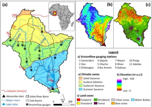
The transboundary VRB is the study area. It covers approximately 415,600 km2across six countries of West Africa. Figure 1 shows the physical and hydroclimatic characteristics of the VRB. The climate is character-ized by a south‐north gradient of increasing aridity and varies from subhumid in the south to semiarid in the north (Dembélé et al., 2019). Climate is driven by the Intertropical Convergence Zone, and four ecoclimatic zones (i.e., Sahelian, Sudano‐Sahelian, Sudanian, and Guinean) can be identified (Figure 1a) based on the average annual precipitation and agricultural features (Food and Agriculture Organization/Global Information and Early Warning System, 1998; Mul et al., 2015). The characteristics of the four ecoclimatic zones are given in Table 1. Actual evaporation exceeds 80% of annual rainfall in the basin (Andreini et al., 2000; De Condappa & Lemoalle, 2009).
The topography is predominatelyflat as 95% of the relief is below 400 m above sea level (Figure 1b). The drai-nage system is composed of four sub‐basins known as Black Volta (152,800 km2), White Volta (113,400 km2), Oti (74,500 km2), and Lower Volta (74,900 km2). The Volta Riverflows over 1,850 km and transits in the Lake Volta formed by the Akosombo dam before draining into the Atlantic Ocean at the Gulf of Guinea (Williams et al., 2016). Land cover (Figure 1c) is dominated by savannah formed by grassland interspersed with shrubs and trees covering about 88% of the basin area. Other land cover types include forest (9%), water bodies (2%), and bare land and settlements (1%).
Figure 1.Physical and hydroclimatic characteristics of the Volta River basin.
Table 1
Characteristics of the Four Ecoclimatic Zones in the Volta River Basin
Ecoclimatic zones Climate class AI(−) P(mm/year) Tavg(°C) Tmin(°C) Tmax(°C)
Sahel Savanna Arid 0.16 [0.12–0.20] 570 [470–610] 29 [29–30] 20 [20–21] 37 [36–38]
Sudano‐Sahelian Semiarid 0.29 [0.16–0.43] 790 [570–980] 29 [28–29] 20 [20–21] 36 [35–37]
Sudanian Savanna Semiarid/dry subhumid 0.47 [0.33–0.98] 1,010 [890–1290] 28 [26–29] 21 [19–23] 35 [32–36] Guinean Savanna Dry subhumid/humid 0.70 [0.49–1.22] 1,190 [1030–1420] 28 [26–29] 21 [19–22] 34 [31–36] Note. The annual mean value (with min‐max range in brackets) is given for each variable. The aridity index (United Nations Environment Programme, 1997) is obtained from the global aridity index database (Trabucco & Zomer, 2018), and the WFDEI data (Weedon et al., 2014) are used for the long‐term (1979–2016) estimation of annual precipitation and air temperature.AI= aridity index;P= precipitation,Tavg= average air temperature;Tmin= minimum air temperature; Tmax= maximum air temperature.
3. Data Sets
The data sets used to set up and run the distributed model for the 2000–2012 period include the basin mor-phological data (elevation, slope, land cover, etc.) and meteorological data (i.e., rainfall and air temperature). In situ streamflow data and complementary data from SRS are used to calibrate and to evaluate the model performance. A description of the data sets with their characteristics and their sources is given in Table 2. The streamflow data were obtained from different organizations (see the Acknowledgements section). Previous work by Dembélé et al. (2019) describes the preprocessing of the streamflow data set, which was quality checked and whose missing data portions were gapfilled.
Concerning the SRS products, the terrestrial water storage (St) anomaly data derived from changes in surface mass, which is related to the Earth's gravity field, is obtained from the Gravity Recovery and Climate Experiment (GRACE; Landerer & Swenson, 2012; Tapley et al., 2004). Over land,Stis the sum of snow, ice, surface water, soil moisture, and groundwater. The data release RL05 (Swenson, 2012) is used in this study. It is a simple arithmetic mean of different solutions from three processing centers: Jet Propulsion Laboratory, Center for Space Research at University of Texas, and Geoforschungs Zentrum Potsdam.
Table 2
Overview of the Modeling Data Sets
Variables Product Spatial resolution Temporal resolution Reference
Model setup Meteorological data
Rainfall CHIRPS v2.0 0.05° Daily Funk et al. (2015)
http://chg.geog.ucsb.edu/data/chirps/ Temperature (average, minimum,
and maximum)
WFDEI 0.5° Hourly Weedon et al. (2014)
http://www.eu‐watch.org/data_ availability
Morphological data
Terrain characteristics (elevation, slope, aspect, flow direction, andflow accumulation)
GMTED 2010 225 m (0.0021°) Static Danielson and Gesch (2011)
https://topotools.cr.usgs.gov/ Soil properties (horizon depth, bulk density,
and sand and clay content)
SoilGrids 250 m (0.0023°) Static Hengl et al. (2017)
https://www.isric.org/explore/soilgrids
Geology GLiM v1.0 0.5° Static Hartmann and Moosdorf (2012)
https://doi.pangaea.de/10.1594/ PANGAEA.788537
Land use land cover Globcover 2009 300 m (0.0028°) Static Bontemps et al. (2011)
http://due.esrin.esa.int/page_globcover. php
Phenology (leaf area index) GIMMS 8 km (0.0833°) Bimonthly Tucker et al. (2005), Zhu et al. (2013)
http://cliveg.bu.edu/modismisr/lai3g‐ fpar3g.html
Model calibration/evaluation In situ data
Streamflow ‐ Point Daily Multiple organizations
(see the Acknowledgements section) Complementary satellite products
Terrestrial water storage anomaly GRACE TellUS v5.0 1° Monthly Tapley et al. (2004), Landerer
and Swenson (2012) https://grace.jpl.nasa.gov/
Surface soil moisture ESA CCI SM v4.2 0.25° Daily Dorigo et al. (2017)
https://www.esa‐soilmoisture‐cci.org/
Actual evaporation GLEAM v3.2a 0.25° Daily Martens et al. (2017),
Miralles et al. (2011) https://www.gleam.eu/ Land surface temperature
(only for model evaluation)
MYD11A2 v6 1 km (0.0083°) 8‐day Wan et al. (2015)
https://lpdaac.usgs.gov/products/ myd11a2v006/
Note. CHIRPS = Climate Hazards Group InfraRed Precipitation with Station data; ESA CCI SM = European Space Agency Climate Change Initiative soil moist-ure; GIMMS = Global Inventory Modelling and Mapping Studies; GLEAM = Global Land Evaporation Amsterdam Model; GLiM = Global Lithological Map; GMTED = Global Multi‐resolution Terrain Elevation Data; GRACE = Gravity Recovery and Climate Experiment; WFDEI = WATCH Forcing Data methodology applied to ERA‐Interim data.
Sakumura et al. (2014) found this ensemble mean product more effective in reducing noise in the Earth's gravity signal compared to the individual products. As the original baseline for GRACE‐derivedStanomaly data is the period 2004–2009, theStdata is converted to a new baseline corresponding to the modeling period (2003–2012) used in this study, by averaging each grid point over the new baseline and subtracting that value from all time steps (National Aeronautics and Space Administration, 2019).
The surface soil moisture (Su) data for a soil layer depth of 2–5 cm is obtained from European Space Agency Climate Change Initiative (ESA CCI; Dorigo et al., 2017). The combined product used in this study is a blended product of both active and passive microwave products derived from scatterometer (European Remote‐Sensing Satellite (ERS), Active Microwave Instrument (AMI) and Advanced Scatterometer (ASCAT)) and radiometer (Scanning Multichannel Microwave Radiometer (SMMR), Special Sensor Microwave/Imager (SSM/I), Tropical Rainfall Measuring Mission (TRMM) Microwave Imager (TMI), Advanced Microwave Scanning Radiometer‐ Earth Observing System (AMSR‐E), WindSat, Advanced Microwave Scanning Radiometer 2 (AMSR2), and Soil Moisture and Ocean Salinity (SMOS)) retrievals (Liu et al., 2012; Wagner et al., 2012). The merging algorithm of the combined product version 4.2 is described by Gruber et al. (2017).
Actual evaporation (Ea) data are obtained from the Global Land Evaporation Amsterdam Model (GLEAM) land surface model that uses satellite data as input (Martens et al., 2017; Miralles et al., 2011). It separately esti-mates the components of terrestrial evaporation (i.e., transpiration, bare soil evaporation, open‐water evapora-tion, interception loss, and sublimation) based on the fraction of land cover types (i.e., bare soil, low vegetaevapora-tion, tall vegetation, and open water) before aggregating them for each grid cell. In GLEAM, potential evaporation (Ep) is calculated based on the Priestley and Taylor (1972) equation and thereafter converted into transpiration or bare soil evaporation using a stress factor, which is a parameter that accounts for environmental conditions limiting evaporation. The stress factor is estimated from microwave vegetation optical depth (i.e., water con-tent in vegetation) and root‐zone soil moisture that is calculated with a multilayer water balance algorithm. The fraction of open‐water evaporation is assumed to equalEp. The Gash (1979) analytical model further refined by Valente et al. (1997) is used to calculate rainfall interception by forests.
Land surface temperature (Ts) data from the Moderate Resolution Imaging Spectroradiometer (MODIS) instrument of the National Aeronautics and Space Administration satellites are used as independent data for model evaluation, and they are not used during model calibration. The daytime product from the Aqua platform is used because that satellite passes over our study region around 13:45 in local time, corre-sponding to the highest daily temperature period with a clear‐sky coverage (Wan et al., 2015).
For a full description of the data sets, the reader is referred to the corresponding data references in Table 2.
4. Experimental Design
4.1. Hydrological Model
mHM (version 5.8) is a spatially explicit (i.e., fully distributed) conceptual model based on numerical approx-imations of dominant hydrological processes per grid cell in the modeling domain (Kumar et al., 2013; Samaniego et al., 2010). The following processes can be represented: canopy interception, snow accumula-tion and melting, soil moisture dynamics, infiltration and surface runoff, evaporation, subsurface storage and discharge generation, deep percolation and baseflow, and discharge attenuation andflood routing. The total grid‐generated runoff is routed to the neighboring downstream cell following the river network using a multiscale routing model (Thober et al., 2019) based on the Muskingum‐Cunge method (Cunge, 1969). mHM uses an MPR technique (Samaniego et al., 2017) to account for the subgrid variability of the basin physical characteristics (e.g., topography, soil texture, geology, and land cover properties). Pedotransfer functions and global parameters are used to link the model parameters (e.g., hydraulic conduc-tivity and soil porosity) to the basin physical characteristics. There are at most 53 global or super parameters (Pokhrel et al., 2008), which are time‐and space‐invariant parameters tuned during the calibration proce-dure. The model uses three different scales of spatial discretization (i.e., grid cell resolution) of the modeling domain corresponding to operation levels. Thefirst scale is used for morphologic data (L0), the second is dedicated tofluxes and states calculation (L1), and the third scale is considered for the meteorological data (L2). L1 should be a multiple of L0 and a submultiple of L2. Three land use and land cover classes are
considered by mHM: forests (e.g., coniferous and deciduous), permeable areas (e.g., grasslands, croplands, and bare soils), and impervious areas (e.g., urban and built‐up areas, water bodies, and consolidated soils).
4.2. Model Implementation
For the current setup of the mHM model, reference evaporation (Eref) is calculated based on the Hargreaves and Samani (1985) method, which only requires temperature data. Following Demirel et al. (2018), a dyna-mically scaling function (FDS) is used to calculate potential evaporation (Ep) to account for vegetation‐ climate interactions and improve spatial estimation ofEp(Bai et al., 2018; Jiao et al., 2017). The approach is based on the concept ofEpcalculation from crop coefficients andEref(Allen et al., 1998; Birhanu et al., 2019). Here theFDS(equation (1)) plays the role of a spatially varying crop coefficient, and it is estimated based on leaf area index (ILA) data. It is formulated as follows:
FDS¼aþb 1−eðc·ILAÞ
; (1)
whereais the intercept term representing uniform scaling,brepresents the vegetation‐dependent compo-nent, andcdescribes the degree of nonlinearity in theILAdependency. The coefficientsa,b, andcare deter-mined during model calibration.
Ep¼FDS×Eref: (2)
Total actual evaporation (i.e., all forms of evaporation including transpiration,Ea) is estimated as a fraction ofEpfrom soil layers and depends on the fraction of vegetation roots and soil moisture availability (Feddes et al., 1976). Soil moisture is calculated following a multilayer infiltration capacity approach using a three‐ layer soil scheme. The depths of the soil layers are 5, 30, and 100 cm. Terrestrial water storage in mHM is calculated per grid cell by summing up all the subsurface water storage (i.e., reservoirs generating soil moist-ure, interflow, and baseflow) and the surface water storage in sealed areas. There is no snowfall in the VRB. In this study, 36 global parameters are determined through model calibration (see supporting information Table S2). The full description of the model and the formulation of the hydrological processes can be found in the work of Samaniego et al. (2010). All morphological data are resampled to a resolution of 1/512° (~200 m at the equator) and the meteorological data to 0.0625° (~7 km). The nearest neighbor technique is used to resample categorical data, while bilinear resampling is used for continuous data. The model is run at daily time step with a spatial resolution of 0.25° (~28 km), corresponding to 619 modeling grid cells in the basin, but taking into account the subgrid variability of the morphological data using the MPR tech-nique (Samaniego et al., 2010; Samaniego et al., 2017). Every modeling grid cell (L1) contains 16 meteorolo-gical grid cells (L2) and 16,384 morpholometeorolo-gical grid cells (L0).
4.3. Model Calibration and Evaluation Strategies
The modeling period spans from 2000 to 2012 and consists of 3 years (2000–2002) model warm‐up period, 6 years (2003–2008) calibration period, and 4 years (2009–2012) evaluation period. Based on data availability and quality in the VRB (Dembélé et al., 2019), 11 streamflow gauging stations are chosen to have a good coverage of the river network (Figure 1), and the calibration is done on them simultaneously to obtain a single‐parameter set for the whole VRB. The domain‐wide calibration, which was proven to give similar performance as the domain‐split calibration (Mizukami et al., 2017), is preferred here because of the limited number of streamflow stations and for seamless spatial pattern representation across sub‐basins (see Figure 1).
Two main calibration approaches are adopted to evaluate the benefit of including spatial patterns in multi-variate parameter estimation with SRS data. Thefirst approach is the streamflow‐only calibration, and the second approach uses multiple SRS data sets in addition to streamflow. In both cases, the formulation of the objective functions follows the Euclidian distance approach in which all elements are equally weighted (Khu & Madsen, 2005); see equation (A1).
4.3.1. Calibration on Streamflow—Benchmark
Thefirst calibration approach is the benchmark calibration case (caseQ) where the hydrological model is constrained with in situ streamflow (Q) data only. An objective functionΦQ(equation (3)) combines the Nash‐Sutcliffe efficiency (Nash & Sutcliffe, 1970) of streamflow (ENS) and the Nash‐Sutcliffe efficiency of
the logarithm of streamflow (ENSlog) presented in equations (A2) and (A3), and it is formulated as Euclidean distance such that it has to be minimized:
ΦQ¼ 1 g∑ g 1 ffiffiffiffiffiffiffiffiffiffiffiffiffiffiffiffiffiffiffiffiffiffiffiffiffiffiffiffiffiffiffiffiffiffiffiffiffiffiffiffiffiffiffiffiffiffiffiffiffi 1−ENS ð Þ2 þ1−ENSlog2 q ; (3)
wheregis the number of streamflow gauging stations present within the modeling domain.ΦQis obtained by equally weighing the streamflow gauging stations, and it ranges from 0, its ideal value, to +∞.
4.3.2. Calibration on Multiple Variables With Spatial Patterns 4.3.2.1. Spatial Pattern Efficiency Metric
The degree of reproduction of the spatial patterns ofEaandSuis quantified with a proposed pattern match-ing metric, denotedESP. The development ofESPis motivated by the need for simplicity and robustness in pattern matching with respect to existing metrics (cf. Koch et al., 2015; Koch et al., 2018). It is a multicom-ponent metric formulated in a way functionally equivalent to the Kling‐Gupta efficiency (cf. equation (A6); Gupta et al., 2009; Kling et al., 2012) and the SPAtial EFficiency metric (SPAEF, Demirel et al., 2018; Koch et al., 2018). It simultaneously assesses the matching of the spatial distribution of grid cells, the relative var-iation, and the strength of the monotonic relationship between the observed and estimated variables. Therefore,ESPis a bias‐insensitive metric that focuses on the patterns of the variables rather than their mag-nitudes. Considering a modeled variable (Xmod) and an observed variable (Xobs) ofnelements,ESPis defined as follows: ESP ¼1− ffiffiffiffiffiffiffiffiffiffiffiffiffiffiffiffiffiffiffiffiffiffiffiffiffiffiffiffiffiffiffiffiffiffiffiffiffiffiffiffiffiffiffiffiffiffiffiffiffiffiffiffiffiffiffi rs−1 ð Þ2þðγ−1Þ2þðα−1Þ2 q ;with (4) rs¼1− 6∑ n 1d2 n nð 2−1Þ; (5) γ¼ σmod μmod σobs μobs; and (6)
α¼1−ERMSðZXmod;ZXobsÞ; (7) wherersis the Spearman rank‐order correlation coefficient withdthe difference between the ranks ofXmod andXobs.γis the variability ratio (i.e., ratio of coefficients of variation) that assesses the similarity in the dis-persion of the probability distributions ofXmodandXobs, withμandσrepresenting the mean and the stan-dard deviation, respectively, andαthe spatial location matching term calculated as the root‐mean‐square error (ERMS) of the standardized values (z‐scores,ZX) ofXmodandXobs(see equations (A4) and (A5)). The z‐score is a standardization of the scale of a distribution that facilitates its comparison with another distribu-tion. Thez‐scores identify and describe the exact location of each observation in a distribution (Gravetter & Wallnau, 2013). For a given variable with values represented spatially as a 2‐D matrix, thez‐scores represent the number of standard deviations the value in each grid cell is from the population mean (Oyana & Margai, 2015). Consequently, forcing thez‐scores ofXmodandXobsto be equal (i.e., minimizing theirERMS) corre-sponds to matching their grid cell locations (i.e., spatial patterns). Finally,ESPis formulated such that it ranges from−∞to 1, which is its optimal value. Contrarily toSPAEF, ESPdoes not require any user‐defined parameter (i.e., number of bins inSPAEF), and it uses a nonparametric correlation coefficient (i.e.,rs), which limits its sensitivity to outliers as opposed to the Pearson correlation coefficient (Legates & McCabe, 1999; Pool et al., 2018; Spearman, 1904) used inSPAEF. A comparison ofESPtoSPAEFis provided in the support-ing information (Figure S40 and Table S3).
4.3.2.2. Multivariate Calibration Strategies
In contrast to thefirst calibration strategy, which only considersQas target variable (caseQ), the second cali-bration strategy involves multiple variables (case MV). The potential improvement of the modeledfluxes and states is estimated by constraining the parameter estimation with a simultaneous combination of three variables from SRS products (St,Su, andEa), in addition toQ. Here the spatial patterns ofEaandSuare used in the multivariate calibration, while the temporal dynamics ofStare averaged over the whole basin due to
the relatively coarse spatial resolution of the GRACE data. The temporal dynamics ofStper grid cell is also assessed during model evaluation. The multivariate objective function ΦMV(equation (8)) is defined as follows: ΦMV ¼ ffiffiffiffiffiffiffiffiffiffiffiffiffiffiffiffiffiffiffiffiffiffiffiffiffiffiffiffiffiffiffiffiffiffiffiffiffiffiffiffiffiffiffiffiffiffiffiffiffiffiffiffiffi ΦQ2þΦSt2þΦSu2þΦEa2 q ;with (8) ΦEa¼1− 1 t∑ t
1ESP Ea;modð Þt;Ea;obsð Þt
; (9) ΦSu¼1− 1 t∑ t
1ESP Su;modð Þt;Su;obsð Þt
;and (10)
ΦSt¼ERMS ZSt;modð Þt;ZSt;obsð Þt
; (11)
wheretis the number of time steps of the calibration period. The subobjective functionsΦEaandΦSu are based on theESP(equation (4)) of modeled and observedEaandSu, whileΦStdenotes the root‐mean‐square error (ERMS) of thez‐scores of the modeled and observed basin‐averagedStanomaly.
Consequently,ΦQensures a reliable prediction of streamflow signatures (i.e., high and lowflows),ΦEaand
ΦSuserve to improve the spatial patterns of the modeledEaandSu, andΦStconstrains the temporal dynamics of the modeledSt, which should contribute to a better prediction of the water balance at monthly and annual scales. In fact,ΦEaandΦSuare calculated such that the spatial pattern efficiencies ofEaandSuare determined over the grid cells at each monthly time step, before averaging them over the calibration period, whileΦStis calculated for the basin‐averagedStover the calibration period. Note that in theERMSmetric (equation (A5)), ndenotes the number of grid cells in the spatial domain when calculatingΦEaandΦSu(i.e.,αinESP), while it corresponds to the length of the calibration period (i.e.,n=t) in the calculation ofΦSt. All constituents of
ΦMV(i.e.,ΦQ;ΦEa;ΦSu;andΦSt) vary in the same range from 0 to ±∞. Therefore,ΦMVhas the same range of values with an optimal value of 0. The dynamically dimensioned search algorithm (Tolson & Shoemaker, 2007) is used for parameter estimation using 3,000 iterations. Daily streamflow data are used for model calibration, while monthly SRS data are preferred to avoid errors due to potential time lags among satellite sensor measurements and model simulations.
4.3.2.3. Contribution of Individual Variables to Multivariate Calibration
Assessing the individual contribution of variables used in multivariate calibration is rarely done, although it can help quantify trade‐offs in modelingflux and states variables (Koppa et al., 2019). Here the contribution of each SRS data set to the multivariate calibration case is investigated with a leave‐one‐out approach. The procedure consists in removing one SRS data type from the calibration case MV and evaluating the predic-tive skill of the model. In addition, multivariate calibration without streamflow data, and thus exclusively based on SRS data, is tested to determine the potential of SRS data for hydrological model calibration in regions where little or no streamflow data are available. Consequently, four additional objective functions (Table 3) are used for multivariate calibration cases withoutEa(case MV‐Ea), withoutSu(case MV‐Su), with-outSt(case MV‐St), and without streamflow (case MV‐Q).
Table 3
Variants of Multivariate Calibration Cases in the Leave‐One‐Out Approach Calibration
case
Calibration variable
Objective function Specificity Equation
number Case MV‐Ea Q,St,Su ΦMV−Ea¼
ffiffiffiffiffiffiffiffiffiffiffiffiffiffiffiffiffiffiffiffiffiffiffiffiffiffiffiffiffiffiffiffiffiffiffiffiffiffi ΦQ2þΦSt2þΦSu2
p
No direct constraint on evaporation (12) Case MV‐Su Q,St,Ea ΦMV−Su ¼
ffiffiffiffiffiffiffiffiffiffiffiffiffiffiffiffiffiffiffiffiffiffiffiffiffiffiffiffiffiffiffiffiffiffiffiffiffiffi ΦQ2þΦSt2þΦEa2
p
No specific constraint on surface soil moisture (13) Case MV‐St Q,Su,Ea ΦMV−St¼ ffiffiffiffiffiffiffiffiffiffiffiffiffiffiffiffiffiffiffiffiffiffiffiffiffiffiffiffiffiffiffiffiffiffiffiffiffiffiffi ΦQ2þΦSu2þΦEa2 p
No direct constraint on deep subsurface processes (14) Case MV‐Q St,Su,Ea ΦMV−Q¼ ffiffiffiffiffiffiffiffiffiffiffiffiffiffiffiffiffiffiffiffiffiffiffiffiffiffiffiffiffiffiffiffiffiffiffiffiffiffiffi ΦSt2þΦSu2þΦEa2 p
Only satellite‐based variables with no direct constraint on streamflow
4.4. Postcalibration Model Evaluation
The predictive skill of the model is evaluated by assessing the transferability of the global parameters across temporal periods and spatial scales obtained by the abovementioned calibration strategies. First, the tem-poral transferability is evaluated following a split‐sample test that consists in assessing performances for a period that is different from the calibration period (Klemes, 1986). Secondly, spatial scale transferability is evaluated by using different grid cell (i.e., pixel) sizes as modeling resolution (Kumar et al., 2013; Samaniego et al., 2010). The global parameters of the model for all calibration cases are obtained for a reso-lution of 0.25° (~28 km, i.e., 619 pixels in the basin), and the same parameters are used to run the model without recalibration at four differentfiner scales: 0.125° (~14 km, i.e., 2,320 pixels), 0.0625° (~7 km, i.e., 8,974 pixels), 0.03125° (~3.5 km, i.e., 35,231 pixels), and 0.015625° (~1.75 km, i.e., 139,494 pixels). The eva-luation data for model parameter transferability are streamflow for streamflow, using the Kling‐Gupta effi -ciency (EKG), andfine‐scaleTsdata to evaluateEa and Su, usingrs, while no high‐resolution data are available forStevaluation.Tsis used as proxy data for the evaluation ofSuandEabecause past studies found significant negative correlation betweenTsandSu(Kumar et al., 2013; Lakshmi et al., 2003; Wang et al., 2007) and a control ofTsoverEa(Boni et al., 2001; Lakshmi, 2000).
Following Biondi et al. (2012), supplemental skill metrics different from those used in model calibration are computed for a thorough model evaluation because every metric has its own limitations (Fowler et al., 2018; Knoben et al., 2019; Santos et al., 2018; Schaefli & Gupta, 2007). In addition toENS,ENSlog,ESP,ERMS, andrs, theEKGis reported for model evaluation.
5. Results and Discussions
The following section presents and discusses the results of model performances for different variables used in the calibration procedure. The results refer to the evaluation period when analyzing the results if not clearly specified. However, both calibration and evaluation results are presented in figures. Hereafter, the SRS data sets are called reference data, as they are not direct observations. Detailed results on model performances for each of the four climatic zones in the VRB are provided as supporting information (Figures S17–S33).
5.1. Model Performance for Streamflow
The model performance for streamflow (Q) at the 11 gauging stations is given in Figure 2. For the calibration period, the meanEKGis 0.67 (ENS= 0.71,ENSlog= 0.72) for the model calibration with onlyQdata (i.e., case
Figure 2.Statistics of model performance for streamflow. The best score of all the metrics is 1. The dots give the mean score, and the bars represent the min‐max range of values for 11 streamflow gauges. The colors correspond to the model calibration cases.
Q). The performance ofQin the calibration period decreases when multiple variables are used to constrain the parameter search. The meanEKGis 0.55 (ENS= 0.57,ENSlog= 0.66) for the multivariate calibration (i.e., case MV), corresponding to a decrease of 18% compared to that in caseQ.
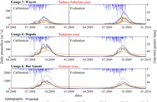
Regarding the other multivariate calibration cases, the best performance with respect toQis obtained in case MV‐Stwith a meanEKGof 0.65 (ENS= 0.67,ENSlog= 0.70), which represents a slight decrease of 3% compared to that in caseQ, while the weakest performance is given by case MV‐Qwith a meanEKGof 0.19 (ENS = 0.33,ENSlog=−0.38). Differences in measurement scales betweenQdata and satellite pro-ducts (i.e., river dimensions vs. pixel size) can justify a low performance for case MV‐Q (see section 5.5). In general, all calibration cases give a good timing of Q with a mean correlation coefficient of r> 0.79, but they underestimate it with a mean bias ofβ< 0.85, except case MV‐Q, which shows over-estimation with a positive bias (β= 1.19). They all show a higher variability ofQthan the observed data, with meanγ> 1.04, except caseQ(γ= 0.98) and case MV‐Q(γ= 0.40), which produce a lower variability. A subset of the hydrographs of three stations from different climatic zones are depicted in Figure 3. More statistics on the model performance along with the complete hydrographs andflow signatures (i.e.,flow duration curves and seasonal streamflow) are provided in the supporting information (Table S1 and Figures S1–S11).
During the evaluation period, as compared to the calibration period, the model performance for the mean EKGdecreases by 2% for caseQ(from 0.67 to 0.66) and case MV‐St(from 0.65 to 0.64) and 90% for case MV‐Q(from 0.19 to 0.02), while it increases by 7% for case MV‐Ea(from 0.61 to 0.65), 12% for case MV‐Su (from 0.56 to 0.62), and 14% for case MV (from 0.55 to 0.63). Considering the meanEKG, case MV performs less well than caseQby 11% on average, which means 18% less during the calibration and 4% less during the evaluation period. The deterioration of streamflow performance in a multivariate calibration setting is also reported in previous studies (Bai, Liu, & Liu, 2018; Livneh & Lettenmaier, 2012; Pomeon et al., 2018; Rakovec et al., 2016). However, this is largely an artefact of Type I error (i.e., falsely accepting poor models; Beven, 2010) induced by theQ‐only calibration, resulting in inconsistency in the representation of processes (Gupta et al., 2012; Hrachowitz et al., 2014). In addition, the performance ofQslightly increases whenEa (+7%) orSt(+11%) are left out of the multivariate calibration with case MV during the evaluation period. Therefore, as shown in Figure 2, the combinationsQ+St+Su(i.e., case MV‐Ea) andQ+Su+Ea(i.e., case MV‐St) are the best for streamflow prediction, while Q+St+Ea(i.e., case MV‐Su) performs similar to Q+St+Su+Ea(i.e., case MV).
Figure 3.Hydrographs at selected stations in different climatic zones for all model calibration cases. Only a subset of the simulation period (2003–2012) is shown for visualization.
5.2. Model Performance for Terrestrial Water Storage
The statistics for the monthly terrestrial water storage (St) anomalies are given in Figure 4. The results per climatic zone is provided in the supporting information (Figure S19). A similar trend in skill scores (i.e., ERMSandr) among all calibration cases is observed in the calibration and evaluation periods with weaker scores during evaluation.
The evaluation period is characterized by a substantial improvement from model case Q (median ERMS= 8.41 cm,r= 0.73) to case MV (ERMS= 7.38 cm,r= 0.81). In general, all multivariate calibration cases reproduce the variability inStbetter than did caseQ. Previous studies also reported improvement ofSt pre-diction in multivariate settings (Chen et al., 2017; Livneh & Lettenmaier, 2012; Werth et al., 2009). The low-est performance increase is observed whenEa(ERMS= 8.21 cm,r= 0.76) orSt(ERMS= 8.18 cm,r= 0.78) is removed from the multivariate setting. The best prediction is obtained with case MV‐Q, yielding median ERMSof 6.65 cm androf 0.84.
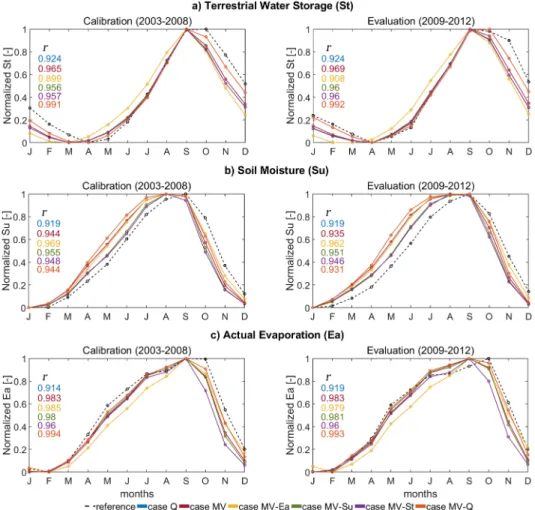
Figure 5a shows the climatology of the basin‐averagedStfor all models. The full monthly time series (Figure S17) and the climatological trends (Figure S18) per climatic zone are provided in the supporting information. The temporal dynamics of the normalized GRACE‐derivedStis well reproduced by all models (r> 0.89) with different degrees of underestimation from September to March, which is a period with little or no rainfall, and slight overestimation from April to June, which is the beginning of the rainy season. All modelsfit well the period July–August, which is the wettest period of the rainy season. In general, case MV‐Eashows the highest deviation from the satellite signal (r= 0.90) followed by caseQ(r= 0.92). Removing spatial patterns ofEafrom the calibration leads to anStoverestimation during the rainy season and an underestimation dur-ing the dry season. The same trend can be observed when onlyQis used for model calibration (i.e., caseQ). TheStsimulation improves in the multivariate calibration includingQ(i.e., case MV,r= 0.97), but the best match is obtained whenQis left out (i.e., case MV‐Q,r= 0.99). When GRACE‐derivedStis excluded from the parameter estimation (i.e., case MV‐St), the model still performs well forStclimatology withr= 0.96. Consequently,Eais the most critical variable for predicting theStsignal in the proposed multivariate cali-bration setting, whileSuis less critical, probably because the GRACE‐derivedStsignal already accounts forSu(Li et al., 2012).
5.3. Model Performance for Soil Moisture
The climatology of the basin‐averaged reference (i.e., ESA CCI) soil moisture (Su) and different modeledSu are depicted in Figure 5b. The maps of climatology (Figures S13 and S14), the full monthly time series (Figure S20), and the climatological trends (Figure S21) per climatic zone are provided in the supporting information. All calibration cases give a good performance (r> 0.91), with a good representation ofSu sea-sonality during both calibration and evaluation periods.
All simulations overestimate the referenceSuduring the rising limb (February–August), corresponding to the increasing rainfall period, and underestimate it during the recession limb (September–January). Simulations that show the highest deviation from the reference during the rising limb, on the contrary, show the lowest deviation during the recession and vice versa. The overall best performance is obtained with case MV‐Ea(r= 0.96), with a better match when the basin is not water limited (i.e., September–January). Case MV‐St and case MV‐Su show similar performances (r ≈ 0.95) with a consistent deviation from the
Figure 4.Statistics of model performance for terrestrial water storage (St). They‐axis is reversed forERMS. The number of
elements per boxplot (n= 52) corresponds to the number of gird cells for GRACE data in the study area. The colors cor-respond to the model calibration cases.
referenceSufor all months, while case MV and case MV‐Qhave similar performances (r≈0.94) but with a betterfit of the referenceSuin the recession limb. It can be inferred thatQis the most critical variable forSu reproduction during the rising limb, whileStand satelliteSuimprove the simulation during the recession limb. Case Q outperforms all multivariate calibration cases when soil water content increases, and it underperforms them when the maximum water content is reached and starts decreasing. The overall lowest performance is given by caseQ(r= 0.92), followed by case MV‐Q(r= 0.93), suggesting thatQ alone is not sufficient for predicting the temporal dynamics ofSu, but it remains useful in the multivariate calibration setting. Surprisingly,Eadoes not bring substantial information to the multivariate prediction ofSu. Contrastingly, Pomeon et al. (2018) obtained a slight improvement inSusimulation (+7%) when using absolute values of satellite Ea in their multivariate calibration. The model performance in reproducing spatial patterns is measured withESP, and its components (i.e.,rs,γ, andα) are summarized in Figure 6a. The results for each month (Figure S41) and for the climatic zones (Figures S22–S25) are provided in the supporting information.
The evaluation and calibration periods depict similar trends when comparing the different metrics (i.e.,ESP, rs,γ, andα). The lowest performance is given by theQ‐only calibration (i.e., caseQ) with medianESP=−0.07 (rs= 0.54,γ= 0.85, andα= 0.13), followed by case MV‐Suwith medianESP=−0.02 (rs= 0.53,γ= 0.84, and
α= 0.16). Case MV shows better performances with medianESP= 0.03 (rs= 0.57,γ= 0.88, andα= 0.19). The best performance even with a low score is given by case MV‐Eawith medianESP= 0.09 (rs= 0.60,γ= 0.93, andα= 0.19), followed by case MV‐Qwith medianESP= 0.05 (rs= 0.58,γ= 0.82, andα= 0.18) and case MV‐Stwith medianESP= 0.02 (rs= 0.55,γ= 0.87, andα= 0.16). RemovingEaorQfrom the multivariate setting results in better performances, while the removal ofStor satelliteSuresults in lower performances.
Figure 5.Climatology of (a) terrestrial water storage, (b) soil moisture, and (c) actual evaporation with the Pearson cor-relation coefficient (r) indicating the performance of all model calibration cases.
Consequently, satellitesSuand Stare the most important variables for improving the spatial patterns of modeledSu. Better simulation ofSuin multivariate settings is also reported by Lopez et al. (2017) using Ea+Sucalibration and by Pomeon et al. (2018) withQ+Eacalibration.
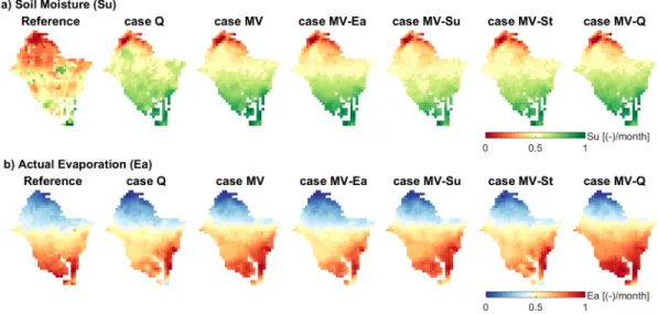
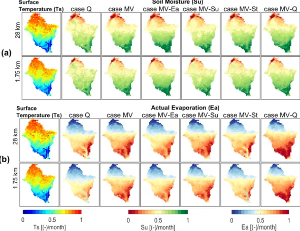
Figure 7.Long‐term monthly average of (a) soil moisture and (b) actual evaporation for all model calibration cases over the simulation period (2003–2012). The reference map represents the satellite product (ESA CCI forSuand GLEAM for Ea). Masked pixels are gaps in satellite measurements or lake areas not modeled in mHM. The values are normalized for
better emphasizing on patterns and using a unique color scale.
Figure 6.Spatial statistics of model performance for (a) soil moisture and (b) actual evaporation. The best score is 1 for all the metrics. The number of elements per boxplot corresponds to the number of months in the calibration period (n= 72) or in the evaluation period (n= 48). The colors correspond to the model calibration cases.
The long‐term monthly average (2003–2012) ofSuis illustrated in Figure 7a. See section 5.5.2 forSu compar-ison withTs. Although the spatial patterns of modeledSuin the multivariate cases are still different from the referenceSu(Figure 7a), they are better than theQ‐only case.
5.4. Model Performance for Evaporation
The climatology of basin‐averaged reference (i.e., GLEAM) actual evaporation (Ea) and different modeledEa are depicted in Figure 5c. The maps of climatology (Figures S15 and S16), the full monthly time series (Figure S26), and the climatological trends (Figure S27) per climatic zone are provided in the supporting information. All calibration cases give a good performance (r> 0.91), reproducing wellEaseasonality during both the calibration and evaluation periods.
The best performance is obtained with case MV‐Q(r= 0.99). In general, all simulations tend to underesti-mateEa. During the rising limb (February–August), corresponding to the increasing rainfall period, the highest deviation is given by case MV‐Ea, although the overall performance is good (r = 0.98). Mismatches are more prominent during the recession limb (September–January), where all modeledEa decrease faster than the reference. The highest deviation is observed when onlyQdata are used for model calibration (r= 0.92), followed by case MV‐St(r= 0.96). It can be inferred that the model case MV‐Stis miss-ing adequate information on the available water amount to be evaporated, which can be obtained from the satelliteStsignal. During the recession period, little to no rainfall occurs in the basin, but a part of antecedent rainfalls is stored in reservoirs and lakes, which represent a major source of land evaporation. It can be argued thatQalone is not sufficient for modelingEa, whileStbrings additional and useful information for simulatingEa, which supports our research hypothesis. The performance of case MV‐Suis similar to that of case MV (r≈0.98), meaning thatSuis not critical for predicting the temporal dynamics ofEa. Moreover, satelliteEaimproves the modeledEaduring water accumulation in the basin (i.e., February–August) and is no longer critical when the basin is not water limited (i.e., September–January). This result suggests that the model can mainly rely on GRACE‐derivedStto reproduceEa. Similar results on the good estimation ofEa with GRACE‐derivedStare found in literature (e.g., Bai, Liu, & Liu, 2018; Livneh & Lettenmaier, 2012; Rakovec et al., 2016). Pomeon et al. (2018) also obtained a higher model performance forEain their multi-variate setting (i.e.,Q+Ea) with mHM in West Africa.
Figure 6b gives the spatial pattern efficiency ofEafor all model calibration cases. The results for each month (Figure S41) and for the climatic zones (Figures S28–S31) are provided in the supporting infor-mation. In general, the performance decreases from the calibration period to the evaluation period, and the modeledEawith all model calibration cases has higher spatial pattern efficiency scores (ESP> 0.25) compared to modeledSu (ESP < 0.1). All multivariate calibration cases outperform theQ‐only calibra-tion, giving the lowest performance with medianESP= 0.28. TheQ‐only calibration gives a good spatial correlation (rs= 0.8) but overestimates the variability (γ= 1.28) and struggles to match the spatial loca-tion of grid cells (α = 0.39) ofEa. The best spatial pattern matching is given by case MV with median ESP = 0.46 (rs = 0.86, γ = 0.95, and α = 0.53). Removing Q from the multivariate setting (i.e., case MV‐Q) results in an underestimation of the spatial variability ofEa, with medianESP= 0.43 (rs= 0.88,
γ= 0.84, and α= 0.52). In contrast, the spatial variability of Eais overestimated for case MV‐Eawith medianESP= 0.45 (rs= 0.85,γ= 1.13, andα= 0.52), while case MV‐Suyields a lower spatial location score with medianESP= 0.42 (rs= 0.85,γ= 0.95, andα= 0.50). The spatial pattern performance ofEa is more sensitive to the removal of St, as shown by case MV‐St with median ESP = 0.35 (rs = 0.81,
γ= 1.07, and α = 0.49). These results indicate that spatial patterns ofSucan improve the spatial pat-terns of Eaand St is critical for reproducing both the temporal and spatial dynamics of Ea. Demirel et al. (2018) similarly reported better spatial pattern performance forEawhen using a multivariate set-ting (i.e.,Q +Ea) compared to that when using theQ‐only calibration.
Figure 7b illustrates the long‐term (2003–2012) monthly average ofEa. See section 5.5.2 forEacomparison withTs. The southern region of the basin, with a subhumid climate, is where the multivariate calibration cases show more differences in spatial patterns compared to caseQ. Besides the south‐north differences, it is interesting to see strong differences in the west‐east variability of the spatial pattern. As the southern part is subhumid (Ea≥70%), small variations inEaare not well represented when the model is calibrated using
onlyQcompared to those in the semiarid northern part. Thesefindings are in agreement with the study of Rakovec et al. (2016), which revealed a more pronounced sensitivity inEaestimation in humid catchments in Europe through a multivariate calibration setting (Q+St). Similar results are obtained by Bai et al. (2016) when testing differentEpformulas in China. Contrastingly, Bai, Liu, and Liu (2018) found that their multi-variate calibration setting (Q+St) benefitted more toEasimulation in dry catchments than in wet catch-ments in China.
5.5. Parameter Transferability Across Spatial Scales 5.5.1. Streamflow Evaluation Across Spatial Scales
The model performance of streamflow in terms of scale transferability of the global parameters is given in Figure 8. The differences in model performance among calibration cases are conserved across spatial scales, with a median coefficient of variation of 1.6% forEKG, 0.1% forr, and 6.4% forβ.
5.5.2. Spatial Pattern Evaluation Across Spatial Scales
Long‐term monthly maps ofSu(Figure 9a) andEa(Figure 9b) are plotted along withTsmaps at various spa-tial resolutions. Here only the coarsest andfinest resolutions (i.e., 28 and 1.75 km) are shown, but the same figures with intermediate resolutions and the spatial pattern efficiency are given in the supporting informa-tion (Figures S34–S37 and S32–S33).
The patterns ofSuis consistent with the patterns ofTsbecause the expectation is that the higher theTs, the lower theSuand vice versa (Figure 9a). For semiarid regions,Ealargely depends on water availability (i.e., rainfall) and is dominant for open water storages. In the VRB,Eadepicts an opposite pattern toTs, which is shown in Figure 9b. The reproduction of bothSuandEain the multivariate calibration cases and across spa-tial scales show more plausible patterns withTs, which are well preserved across scales with higher consis-tency, than their representation with caseQ. The maps of the temporal correlation per grid cell are provided in the supporting information (Figures S35 and S37).
5.6. Benefit of Spatial Patterns and Data Types in Multivariate Calibration 5.6.1. Analysis of the Lake Volta Region
Evidence of the benefit of multivariate calibration with SRS data is exemplified in Figure 10 by zooming‐in on the Volta Lake region in the southern part of the VRB (cf. Figure 1). Notwithstanding that mHM does not have a lake module, it is nicely noticeable that the model represents the heterogeneity in spatial patterns with the multivariate calibration cases being better than the Q‐only calibration case. As it should be
Figure 8.Statistics for model parameter transferability across spatial scales for streamflow performance for all calibration cases. The dots give the mean score, and the bars represent the min‐max range of all values for 11 streamflow gauges. The colors correspond to the model calibration cases.
expected from theTspatterns, case MV shows higherSuandEaover the Lake Volta but with lowerEain its surroundings. This improvement in spatial patterns is not observed with caseQ, confirming the limitations of theQ‐only calibration and emphasizing the importance of patterns of SRS data for model calibration. Moreover, it can be inferred from the results thatStis the most important variable for representing the lake area, whileQis the less critical variable.
Figure 9.Long‐term monthly average of land surface temperature compared to (a) soil moisture and (b) actual evapora-tion for all model calibraevapora-tion cases over the simulaevapora-tion period (2003–2012) at various spatial resolutions. The values are normalized for better emphasizing on patterns and using a unique color scale.
Figure 10.Comparison of the spatial patterns of (tow row) soil moisture and (bottom row) actual evaporation with land surface temperature (first map from left) in the Volta Lake region. TheTsmap used as benchmark shows the Lake
Volta depicted in dark blue with the lowest temperature in the region. The ability of the mHM model to highlight the lake area is assessed with the patterns ofSuandEafor all model calibration cases.
5.6.2. Comparison of the Multivariate Calibration Cases to the Benchmark
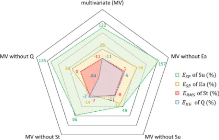
Figure 11 gives the gain or loss in model performance with different multi-variate model calibration cases compared to theQ‐only calibration case (i.e., the benchmark).
In general, the multivariate calibration cases show higher model predic-tive skill for many components of the hydrological system (i.e.,Q,St,Su, andEa) when compared to theQ‐only calibration. The decrease in the model performance forQis usually counterbalanced with an increase in performance forSt,Su, andEa, which might simply be the result of a solu-tion to the artifacts caused by theQ‐only calibration. These results reveal that the simulation of spatial patterns ofSubenefits most from the multi-variate settings, followed by the simulation of Ea and St, while the decrease inQperformance varies widely depending on the multivariate calibration cases. A summary of the importance of each variable in pre-dicting the others (i.e.,Q,St,Su, andEa) is given in Table 4.
The most determinant variable for streamflow prediction in a multivariate setting is streamflow itself, similarly forSu, while it isEaforSt, andStfor Ea. Zeng and Cai (2016) also found thatStcontrols the temporal variability ofEa. Surprisingly,Eais the less critical variable forSuprediction. However, it is worth stressing that only the spatial patterns of satelliteEais exploited here. Moreover,Eacalculation in the model setup might be a reason of the limited contribution of satelliteEainSuprediction. TheEpcalculation (cf. section 4.2) is done with time‐variant and gridded leaf area index data that imposes heterogeneity on modeledEa(Birhanu et al., 2019). Consequently, additional contribution from the satelliteEainSuprediction is expectedly limited in case the leaf area index data are in agreement with the satellite Ea. Moreover, not explicitly weighting the components of the multivariate objective function might have led to implicit weighting, which led to the artifact that some variables are not very good predictors for themselves.
5.7. Summary and Outlook
This work is a follow‐up on several recent studies on multiobjective calibration and spatial pattern improve-ment in hydrological modeling (e.g., Demirel et al., 2018; Koch et al., 2018; Nijzink et al., 2018; Stisen et al., 2018; Yassin et al., 2017; Zink et al., 2018). The proposed multivariate calibration approach is a step forward in improving the realism of hydrological model predictions (Baroni et al., 2019; Clark et al., 2015; Rakovec et al., 2016) because not only a reliable temporal dynamic in the modeling objective but also plausible spatial patterns of several hydrological processes simultaneously are sought for. A key element of our study is the assessment of the plausibility of spatial patterns of soil moisture and evaporation with independent data of land surface temperature not used during the model calibration. With respect to the obtained perfor-mances, it can be concluded that spatial patterns of satellite data are a highly relevant and robust feature that can be used in multivariate calibration to improve the overall representa-tion of the hydrological system even with trade‐offs among the variables, which thereby confirms our research hypothesis.
A rigorous comparison of the proposed bias‐insensitive metric with other spatial pattern metrics is left for future work. Further investiga-tions can focus on setting a threshold for the acceptability of the mod-eled spatial patterns, which was not required here as the goal was to check the increase or decrease of spatial pattern performance rather than determining whether the patterns are good or bad in an absolute sense, when switching between streamflow‐only and multivariate calibration cases.
Our methodology lacks in situ data for model evaluation, except stream-flow. However, in situ measurements of soil moisture, evaporation, and terrestrial water storage at a large scale are rather rare (Vereecken et al.,
Figure 11.Relative difference in performance of multivariate (MV) calibra-tion cases compared to Q‐only calibration case. For every MV case, the values on the line from each vertex to the center of the polygon give the relative difference in performance with theQ‐only calibration case, for all variables (i.e.,Q,St,Su, andEa).
Table 4
Importance of Different Variables in Predicting Others in a Multivariate Calibration Setting
Predictors
Predictands
Temporal dynamics Spatial patterns
Q St Ea Su Ea Su
Q ++++ + ++ +++ + +
St ++ ++ ++++ +++ ++++ ++
Ea ++ ++++ +++ + ++ +
Su ++ + + +++ +++ +++
Note. The degree of importance is as follows: low (+), moderate (++), high (+++), and very high (++++).
2008; Zink et al., 2018) and are also subject to uncertainties due to the nonuniformity of the data collection in space (Stisen et al., 2011). As we focus on spatial pattern assessment in this study, satellite data remain the only possible option for our large study area in West Africa, where ground measurements are a luxury (Dembélé et al., 2019).
The presented multivariate calibration reveals trade‐offs among the objective functions for streamflow and for satellite data. However, trade‐offs cannot be avoided as they originate from errors in input data, model structure, and lack of knowledge of the hydrological system (Bergström et al., 2002; Gupta et al., 1998; Yassin et al., 2017). Moreover, it was a deliberate choice to equally weight the components of the multivari-ate objective function (equation (4)) because no prior knowledge on the importance of each variable was available, and it was an objective of this study to know their contributions in the calibration procedure. In such situation, the default choice is to weight them equally (Bergström et al., 2002; Stisen et al., 2018). Weights are sometimes assigned to objective function components by iterative optimization testing different weights, which is, however, computationally demanding. It is also possible to transform the components of the multivariate objective functions to solve differences in their magnitudes (Madsen, 2003; Zink et al., 2018), but the effects of such transformations on the calibration procedure are unknown and they are not required if the metrics are dimensionless or of the same order of magnitude (Bergström et al., 2002). For completeness, Pareto plots showing the absolute values and the trade‐off among the used objective functions are provided in the supporting information (Figures S38 and S39).
The climatic inputs influence somehow the spatial variability of the hydrological processes due to the aridity gradient in the VRB. The detailed results are valid for the VRB, but they can be generalized to regions with similar hydroclimatic characteristics. However, the applicability of the proposed multi-variate calibration framework is, in principle, universal, as long as a DHM is used and spatial data sets are available. Further research can explore the applicability of the presented multivariate calibration strategies in different hydroclimatic regions with different spatial data sources, and different DHMs to understand how the model structure interacts with the performance of different calibration strategies. Choosing an adequate hydrological model (Addor & Melsen, 2019) is key to any good experiment. The MPR scheme used in mHM might have facilitated to some extent the reproduction of spatial pat-terns, but the MPR scheme can be similarly implemented with other models as demonstrated by pre-vious studies (e.g., VIC and PCR‐GLOBWB models; Mizukami et al., 2017; Samaniego et al., 2017). A sensitivity analysis to identify the model parameters that influence the representation of spatial patterns is a recommended outlook.
Future methodological developments could in particular focus on improved formulation of the multiobjec-tive functions inspired by previousfindings on the following topics:fitting of lowflows and system signa-tures (Fowler, Peel, et al., 2018; Hrachowitz et al., 2014; Krause et al., 2005; Pushpalatha et al., 2012), gauge measurement weighting (Madsen, 2003), or subperiod calibration (Gharari et al., 2013). Additional key questions to address in this context include the model structural deficiencies (Gupta et al., 1998; Gupta et al., 2012) and the uncertainties of modeling data sets (i.e. input, calibration, and evaluation data), which can lead to erroneous model rejection (Beven, 2010, 2018, 2019b).
The above efforts in model improvement are particularly important for prediction in a changing environ-ment (Fowler et al., 2018), and they can set avenues for prediction in ungauged basins solely from space.
6. Conclusion
This study presents a calibration approach using multiple data sources simultaneously, with the specificity of integrating only spatial patterns of satellite remote sensing data in the parameter estimation procedure. A bias‐insensitive and multicomponent metric is proposed for spatial pattern matching. The study is carried out in the Volta River basin in West Africa. Results reveal the benefit of the multivariate calibration setting over the traditional calibration using only streamflow data. The mainfindings are as follows:
• Streamflow is a necessary variable, but alone it is not sufficient for reliably reproducing other hydrological fluxes and states.
• Spatial patterns of satellite data, without the absolute values, can be incorporated in the calibration pro-cedure with bias‐insensitive metrics.
• Multivariate calibration based on streamflow and satellite data can improve the overall representation of the hydrological system and thereby increase the model predictive skill.
• The reduction in streamflow performance in a multivariate setting is largely compensated by the gain in performance for other hydrological processes (i.e., terrestrial water storage, soil moisture, and evaporation). We advocate for the adoption of multivariate calibration procedure focusing on spatial patterns in distribu-ted hydrological models because it is a robust approach for addressing equifinality, reducing uncertainties, and enhancing the predictive skill of hydrological models in a changing environment.
Appendix A: Equations
Euclidean Distance
The Euclidian distance (DE) between two pointsXandYof coordinates (x1,x2,…,xn) and (y1,y2,…,yn) in an n‐dimensional space (Upton & Cook, 2014) is given by
DE¼ ffiffiffiffiffiffiffiffiffiffiffiffiffiffiffiffiffiffiffiffiffiffiffi ∑n iðxi−yiÞ 2 q : (A1)
Nash
‐
Sutcliffe Ef
fi
ciencies
The Nash‐Sutcliffe efficiency (Nash & Sutcliffe, 1970) of streamflow (ENS) and the Nash‐Sutcliffe efficiency of the logarithm of streamflow (ENSlog) are formulated as follows:
ENS¼1−∑ t 1ðQmodð Þt−Qobsð Þt Þ2 ∑t 1 Qobsð Þt−Qobs 2 (A2) and ENSlog¼1−∑ t
1½logðQmodð Þt Þ−logðQobsð Þt Þ 2
∑t
1 logðQobsð Þt Þ−logðQobsÞ
h i2 ; (A3)
whereQmodandQobsare the modeled and observed streamflow, respectively, andtis the number of time steps.ENSandENSlogrange from−∞to their perfect score, that is, 1. These two metrics are used as skill scores to identify and discard parameter sets that provide implausible representations of the system and to subsequently better predict both high and lowflows (Krause et al., 2005; Oudin et al., 2006; Pushpalatha et al., 2012; Santos et al., 2018).
z
‐
Scores and Root
‐
Mean
‐
square Error
The standardized values (z‐scores,ZX) ofXmodandXobsand the root‐mean‐square error (ERMS) of a modeled variable (Xmod) and an observed variable (Xobs) ofnelements, are defined as follows:
ZX¼X−μ
σ (A4)
and
ERMSðXmod;XobsÞ ¼
ffiffiffiffiffiffiffiffiffiffiffiffiffiffiffiffiffiffiffiffiffiffiffiffiffiffiffiffiffiffiffiffiffiffiffiffiffiffiffi 1 n∑ n 1ðXmod−XobsÞ 2: r (A5) whereμandσare the mean and the standard deviation of a given variableX, respectively.
Kling
‐
Gupta ef
fi
ciency
The Kling‐Gupta efficiency (EKG) was introduced by Gupta et al. (2009) and modified by Kling et al. (2012) to avoid some limitations ofENS.EKGcombines correlation, bias, and variability measures and is defined as follows: