Image Processing Using Dataflow Techniques

(1)

JINGUI LI

IMAGE PROCESSING USING DATAFLOW TECHNIQUES

Master of Science thesis

Examiners: Prof. Jarmo Takala and Prof. Shuvra Bhattacharyya

Examiners and topic approved by the Faculty Council of the Faculty of Electrical and Computing

(2)

i

ABSTRACT

JINGUI LI: Image Processing Using Dataflow Techniques Tampere University of Technology

Master of Science thesis, 45 pages July, 2017

Master’s Degree Programme in Information Technology Major: Pervasive Computing

Examiner: Prof. Jarmo Takala and Prof. Shuvra Bhattacharyya

Keywords: image processing, hardware design, dataflow graph, LIDE-C, LIDE-V, Verilog

Corner detection is an important task in digital image processing. Corner detec-tion algorithms are widely used in pattern recognidetec-tion, image mosaicing, modetec-tion detection, etc. The implementations of such algorithm in software/hardware can be challenging. One classical algorithm for finding corners in images is proposed by Harris and Stephens in 1988, commonly known as Harris corner detection al-gorithm; There have been different implementations of the algorithm in OpenCV and on FPGA. The implementations of the algorithm in hardware have been rela-tively less, and most importantly the architectures of the algorithm on FPGA have relatively been unexplored.

LIDE, created at University of Maryland, College Park, is a light-weight dataflow environment for rapid prototyping of DSP systems using dataflow techniques. The framework in C programming language is called LIDE-C, in Verilog HDL is called LIDE-V. This light-weight framework makes modeling of DSPs easy in both software and hardware. It is platform- and language-agnostic. This thesis work models the application both in LIDE-C and LIDE-V, our emphasis is, however, to propose multi-architecture corner detection Harris algorithm in LIDE-V. In LIDE, computations are distributed to different computation nodes in dataflow graphs. Each node is called actor in LIDE, and each actor has different modes of computation. Depending on how we construct a dataflow graph for an application and how we design actors of a dataflow graph, we easily create different implementations for the same algorithm. In this thesis, different hardware architecture of the Harris algorithm will be pro-posed with different latency, resource usage, and throughput characteristics. Our preliminary results reveal, among other things, that unfolding for the non-max sup-pression actor not only improve performance but also decrease resource usage.

(3)

ii

PREFACE

The project, in which I have done my thesis, is a joint project between Tampere University of Technology and University of Maryland, College Park, USA. It has been a great honor to work with people from University of Maryland (UMD), College Park, USA. I feel grateful that my thesis was funded by Tampere University of Technology (TUT).

I started working as a research assistant for Prof. Jarmo Takala in summer 2015, he hired, helped, and patiently guided me. At the time, I knew virtually nothing about hardware verification. I learned a very important lesson as he led me patiently through puzzles. I have enjoyed working for him as much as I enjoyed listening attentively as a student in his DSP Implementations’ lectures.

I would also like to thank Prof. Bhattacharyya for guiding, directing, and helping me throughout my thesis implementation process. I have learned important problem-solving techniques and various, but not limited to, programming techniques as I followed his directions.

It could have been difficult, if not impossible, for me to finish my thesis without the help of so many people. I would like thank PhD student Li Lin at UMD for being a source of inspiration along the way. I would like to thank Doctoral student Timo Viitanen at TUT for always patiently answering my questions. I also want to thank my colleagues Muazam Ali and Renjie Xie for all the interesting discussions. Above all, I am deeply indebted to my parents, Yang and Li. Thanks for striving to provide the best education there was for me. I also want to thank my sister for supporting me in many ways.

Tampere, July 21st, 2017 Jingui Li

(4)

iii

ABBREVIATIONS

LIDE DSPCAD Lightweight Dataflow Graph Environment

DICE DSPCAD Integrative Command Line Environment

DFG Dataflow Graph

DSP Digital Sigal Processing

HDL Hardware Description Language

ADC Analog-to-Digital Converter

DAC Digital-to-Analog Converter

FIR Finite Impulse Response

(7)

1

1. INTRODUCTION

A signal is a function of independent variables such as time, distance, pressure, position, and temperature [1]. A signal can be analog or digital. If a signal is continuous in time and amplitude, it is said to be analog. In contrast, if a signal is defined only at some discrete points and can be represented using finite number of bits in computers, it is said to bedigital. The definition of digital signal, depending on the context, can vary. This thesis work focuses on digital signal processing, and the definition of digital signal refers to the one mentioned above.

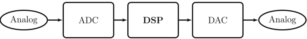
Digital signal processing (DSP) is application of mathematical operations on digital signals. A typical signal processing system is shown in the Fig. 1.1.

Analog ADC DSP DAC Analog

Figure 1.1 A signal processing system

There are analog to digital converter (ADC), digital signal processing (DSP), and digital to analog (DAC) in the system. ADC and DAC modules are important as conversions from analog to digital and from digital to analog are sometimes indispensable. The ADC, which deals with sampling of analog signals, needs to sample the analog the signal so that there is no aliasing. According to Nyquist-Shannon sampling theorem, the sampling frequency should be at least twice of the frequency of highest component in the original signal [2, 3]. The real sampling frequency is usually set much higher than this theoretical lower bound. The DSP part deals with digital signal addition, subtraction, multiplication, division or a combination of the above. The operations on digital signals in one domain, say time domain, is equivalent to some operations applied to the signal in another domain. DSP has a lot of advantages over analog signal processing [4].

(8)

pro-1. Introduction 2 cessing, has many applications in our life. It is widely used in machine learning system, pattern recognition, object detection, etc. A very good example where a sophisticated digital image processing system is involved is cars with auto-pilot system. An auto-pilot system is a fairly complicated system, the digital image pro-cessing part alone is far beyond the scope of this thesis. We might wonder, how on earth can the system know to slow down when it "sees" a speed limit sign, or how can it tell where the car should stay on the road, etc. The system should be able to respond accordingly when it "sees" different traffic signs or road conditions, this is where digital image processing comes into play; Another example which we might see or use everyday is image filtering, oftentimes we see people posting interesting filtered photos on social media. It is impossible to see this new way of life without the knowledge of digital image processing.

In the scope of this thesis work, we mainly focus on an application in digital image processing. The application, called Harris corner detection algorithm, is for finding corners in digital images. The goal is to implement the algorithm efficiently and rapidly. Implementation of DSP in software and hardware can be a very challenging task. In this thesis work, a framework called LIDE for experimenting with dataflow design techniques will be applied. The framework in the C programming language is called LIDE-C, the framework in Verilog HDL is called LIDE-V. Implementations of the algorithm in LIDE-C and LIDE-V will be the topic. The focus, however, will be hardware (LIDE-V) implementation.

The thesis work is arranged like this: Chapter 1 is introduction part. In chapter 2, we will talk about the theoretical background of this thesis work. Chapter 3, LIDE and DICE will be introduced. Chapter 4 will be focused on LIDE-C implementation of the algorithm. Chapter 5 will be about different LIDE-V implementations of the algorithm. In the last chapter, we will draw conclusions and about future work.

(9)

3

2. THEORETICAL BACKGROUND

This chapter provides the theoretical background of the thesis. We will first focus on digital image processing, then we will proceed to a common task in digital image processing – edge detection. The algorithm considered in this thesis work is the Harris algorithm for corner and edge detection. At the end, we will be addressing graphical representations of DSP algorithms.

2.1 Digital Image Processing

Digital image processing, as a sub-field of digital signal processing, is everywhere in our life. The ever-increasing ability for capturing information for human interpreta-tion and processing of image data for storage, transmission, and representainterpreta-tion for machine perception have made image processing more and more popular [5]. Ev-ery time we apply filtering effect on a photo captured by our smart phone, there is digital image processing involved. But the applications of digital image processing is far beyond what we can see. Digital image processing techniques are widely used in machine vision, pattern recognition, video encoding, feature extraction, medical image processing, etc.

2.1.1 Digital Image Representation

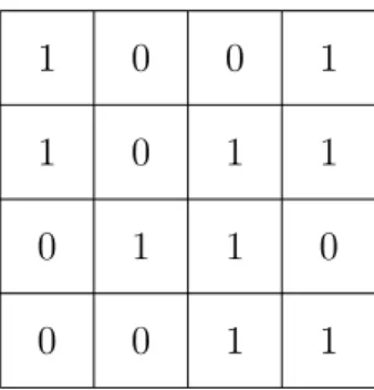
A digital image is a numeric representation of a two-dimensional image. Each digital image is composed of indivisible points called pixels. There is an intensity value at each pixel. Intensity values are encoded using a number of bits in digital computers. An illustration of a digital image (binary image) is shown in Fig. 2.1

A binary image is a type of digital image, the intensity value of each pixel can be one of two values (colors). Colored image processing is getting more and more popular, Each pixel is a vector of three values, namely R, G, B values, where R, G, B refers to

(10)

2.1. Digital Image Processing 4

1 0 0 1

1 0 1 1

0 1 1 0

0 0 1 1

Figure 2.1 A binary image in computers

red, green and blue respectively. By carefully "mixing" red, green, and blue colors, we can create an array of colors. Apparently, encoding a colored image of the same size requires more storage space than encoding a binary image.

2.1.2 Image Gradient

One important concept in digital image processing is image gradient. Gradient, simply put, is the rate of change. If we think of a digital image as a terrain and the intensity value at each point as height, then image gradient at a certain point is the uphill or downhill [6]. Mathematically, gradient of a two dimensional function f(x, y)can be formulated as:

∇f = ∂f

∂x~i+ ∂f

∂y~j, (2.1)

where~i and~j refer to unit vectors on x and y axial. To get the partial derivative of f(x, y) in one direction, we need to know how fast the f(x, y) changes when we change an infinitesimal amount in that direction. It is impossible in the case of digital image as the "function" is only defined at some discrete points in two dimensional space. The image gradient we refer to is basically the approximation of derivative as if there was a continuous function defined at the discrete points. Mathematically, a digital image is a two dimensional function whose definition exists only at some discrete points.

2.1.3 Image Convolution

Image convolution is a two dimensional operation applied on images. To perform image convolution, we need an input image and akernel. A convolution kernel in the

(11)

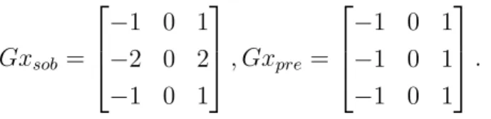
2.2. Edge Detection Algorithms 5 context of image processing, is also called convolution matrix or mask, is a matrix used for convolving with the input image. Below are two kernels, Sobel and Prewitt kernel, commonly used for horizontal gradient approximation.

Gxsob =    −1 0 1 −2 0 2 −1 0 1   , Gxpre =    −1 0 1 −1 0 1 −1 0 1   . (2.2)

The Fig. 2.2 illustrates how image convolution works. To perform convolution, we extract a matrix of the same size as the kernel from the input image. Then we do element-wise multiplication, in the figure we need to perform 16 multiplications. The final step is to sum all the multiplication results, and the sum corresponds to one value in the output image. To calculate all the pixel values in the output image, we need slide a window of the same size as the kernel through the input image. Depending on the application, the rate at which we slide the window is different. In the preparation of the thesis, the step was set to one pixel. For the elements nearby the edges, we applied zero-padding to make it possible to convolve.

Figure 2.2 Convolution mask (left), input image (middle) and output image (right)

2.2 Edge Detection Algorithms

One task in image processing, besides filtering, is to find boundaries in images. Finding boundaries (edges) is fundamental for feature detection, pattern recogni-tion, and computer vision systems. Edge detection techniques can even be used in information compression. A boundary or edge, can be intuitively defined as the position where there is abrupt change of pixel intensity value. It may seem straightforward to find an edge, as we easily notice a sharp change in images, but

(12)

2.2. Edge Detection Algorithms 6 developing an algorithm for finding edges in a way that is stable, insensitive to noise, computationally-nonintensive is challenging. There are so many algorithms for finding edges in an image, each algorithm has its characteristics, advantages, and drawbacks. Edge detection algorithms can be broadly categorized as gradient based and Laplacian based.

Here we briefly introduce the Sobel, Prewitt, and Canny edge detection algorithm.

Sobel Edge Detector

The Sobel edge detection algorithm was developed by Sobel and Fredman, they presented the idea in 1968 [7]. The algorithm uses two 3 by 3 kernels to convolve with the original image to calculate horizontal and vertical derivative approximation. The horizontal kernel and vertical kernel are below:

Gx =    −1 0 1 −2 0 2 −1 0 1   , Gy =    1 2 1 0 0 0 −1 −2 1   .

The results of horizontal and vertical convolution will be the used to calculate a gradient value at a position. The formula for calculating the approximation of gradient Gradis:

Grad=

q G2

hor+G2ver,

where Ghor and Gver refer to horizontal and vertical derivative approximation

re-spectively. The direction of gradient at a place is determined by the formula: θ = arctan(Ghor

Gver

).

In practice, the implementation of square root calculation is usually replaced by the following formula to reduce computation time (resources)

Grad≈ |Ghor|+|Gver|.

This simplification greatly reduces area in hardware implementations, also it is com-paratively easier to implement.

Prewitt Edge Detector

(13)

2.2. Edge Detection Algorithms 7 to implement. The kernels for horizontal and vertical gradient approximation are:

Gx =    −1 0 1 −1 0 1 −1 0 1   , Gy =    −1 −1 −1 0 0 0 1 1 1   .

Since the kernels are different, the spectral response is different. In the preparation of this thesis, both Sobel and Prewitt kernels were used for implementations.

Canny Edge Detector

The Canny edge detector was proposed by John Canny in [8] in 1986. The edge detector is widely deemed as the one of the most widely-used edge detection al-gorithms. The algorithm works in more complex fashion compared to Sobel and Prewitt operators. The steps for running the algorithm are below:

1. Gaussian smoothing

The basic idea behind Gaussian smoothing is very simple, we use a kernel which approximates a continuous two-dimensional function G(x, y) = ₂_πσ12e

−x2+y2 2σ2 _to

convolve with the image. The purpose of Gaussian smoothing is to reduce noise in the image. When it comes to implementation, the kernel can be a 5 by 5 kernel of the following form:

KGaussian =         1 4 7 4 1 4 16 26 16 4 7 26 41 26 7 4 16 26 16 4 1 4 7 4 1        

The criteria for approximating Gaussian kernel is unclear. 2. Gradient approximation

We calculate derivative approximation for the smoothed image. The operators for gradient approximation can be Sobel, Prewitt, or even others. The proce-dure for calculating a gradient value at a position is the same as mentioned previously. Here, often times we use the sum of absolute values to avoid square root calculation.

3. Non-max suppression

Non-max suppression, as the name suggests, "suppresses" non-max gradient values. The purpose is to make the edges more obvious in the output image.

(14)

2.3. Harris Corner Detection Algorithm 8 We keep the max gradient value from a window and the rest of gradient values will be set as zero.

4. Double threshold

Due to noise in the image, we need to "filter" out fake edges. To that end, we use double threshold. We predefine two threshold valuesThigh and Tlow. If

gradient value at a place is higher thanThigh, we mark it as a strong edge pixel.

If gradient value at a place is lower than Tlow, it is "suppressed". If the value

is betweenThigh and Tlow, it is marked as a weak edge pixel.

5. Edge tracking

After the previous step, there are probably still some fake edge pixel among weak edge pixels. The purpose of the step is to remove fake edge pixels. Usually real edge pixels are connected to strong edge pixels. The implication is by removing unconnected weak pixel values, we effectively remove false edge pixels.

The number of edge detection algorithms is far beyond three, the listed algorithms are somehow related to this thesis work. Maini and Aggarwal provide comparisons of different edge detection algorithms in [9].

2.3 Harris Corner Detection Algorithm

The algorithm which we implemented was proposed by Harris et al. in [10]. Unlike edge detection algorithms, the algorithm attempts to find the corners in the input image. But the procedure for finding corners is to a great extent similar. Now the question is: what is a corner?

A corner is the intersection of two edges. To make it easy to understand, if the horizontal and vertical derivatives are very large at a place we find a corner. Suppose we take a small window from an image, let us denote Ix and Iy as horizontal and vertical derivative respectively. If the following sum ( 2.3) leads to a large value,

X

Ix2+XIy2 (2.3)

we can say we find a corner. This happens only when the horizontal and vertical gradients are large. But what happens when we rotate a corner such that the horizontal and vertical gradients are both not so pronounced? In this case, we

(15)

2.4. DSP Algorithm Representations 9 consider the eigenvalues of the following gradient covariance matrix 2.4:

G= " P Ix2 P IxIy P IxIy P Iy2 # . (2.4)

If the eigenvalues of the matrix are large, we likely have a corner. Harris algorithm is really just generalization of the case when a horizontal and vertical edge intersect.

2.4 DSP Algorithm Representations

DSP algorithms are usually non-terminating, the representation of them can take different forms. For example, a 4-tap FIR filter can be represented compactly using the following formula:

y(n) = a0x(n) +a1x(n−1) +a2x(n−2) +a3x(n−3). (2.5)

Transforming such a formula to a program is fairly straightforward, but it does not help in intuitively understanding and identifying the characteristics of the algorithm. We resort to graphical representations of DSP algorithms for a better understanding of algorithm properties.

Four types of graphical representations, block diagram, signal flow graph (SFG), data flow graph (DFG), and dependency graph (DG), are used for representing DSP algorithms in the form of directed graph. Different graphical representations of DSP algorithms are shown in [11].

Block Diagram

Block diagram is a directed graph consisting of computation nodes and edges. The block diagram of the above-mentioned 4-tap FIR filter is shown in Fig. 2.3. There are four types of elements: adder, multiplier, unit delay, and edge in Fig. 2.3. A block diagram explicitly reflects the functionality of a system and various block diagram can be derived for the same system [11].

Signal Flow Graph

Signal Flow Graph (SFG), is basically a collection of nodes and edges. Nodes rep-resent computational tasks. The input node x[n] is called source node, the output nodey[n] is calledsink node. The SFG in Fig. 2.4 can be transformed into different

(16)

2.4. DSP Algorithm Representations 10 x[n]

z−1 _z−1 _z−1

a0 a1 a2 a3

y[n]

Figure 2.3 Block diagram of the 4-tap FIR filter

forms. For a single-input-single-output system, we can apply transposition to the original graph.

x[n]

y[n]

z−1 _z−1 _z−1

a0 a1 a2 a3

Figure 2.4 SFG representation of the 4-tap FIR filter

Dataflow Graph

Dataflow Graph representation is the representation we focus on in this thesis. DFG is a directed graph consisting of edges and computation nodes. On each edge, there is a non-negative delay associated with it. A trivial example for representing

A

B D

Figure 2.5 A trivial example of DFG

computation

y(n) =ay(n−1) +x(n)

is represented in Fig. 2.5. The graph is fairly abstract considering the amount of information connoted. DFG reflects the data-driven property of DSP systems. A node can carry out computation whenever there is enough data available, in the following chapters we will see that a node can "fire", i.e., carry out computation, when it is "enabled".

(17)

2.4. DSP Algorithm Representations 11 In the DFG in Fig. 2.5, there is one delay on the edge from A toB as denoted by Don the edge. The delay implies that there is intra-iteration precedenceconstraint, while on the edge from B toAthere is inter-iteration precedenceconstraint as there is no delay on the edge.

Depending on the granularity of computation nodes, a DFG can beatomicor coarse-grain. An atomic DFG is a DFG whose computation nodes are indivisible, the operations are basic operations like addition, multiplication, etc. In a coarse-grain DFG, a node is a task consisting several indivisible operations. In this thesis, we mainly deal with coarse-grain DFG.

A DFG is said to be synchronous if input and output ratio is constant, i.e., con-sumption to production ratio is constant. A synchronous DFG (SDFG) can be used to describe multi-rate system, the Fig. 2.6 shows an example of a multi-rate system. Note: the numbers in the below graph denote the number of equivalent connections (edges). The numbers on the edges refer to consumption or production rate. Take

A B C

1 3 5 2 3 2

Figure 2.6 A multi-rate system

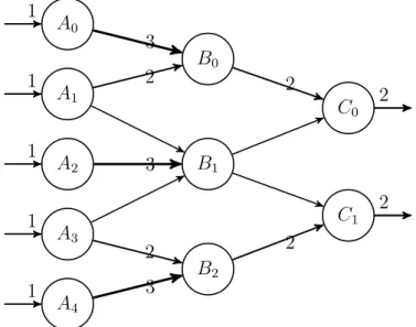
the node A as an example, it consumes 1 sample and produces 3 samples. We can use a technique called unfolding to transform the multi-rate system to single rate system. An unfolded graph of Fig. 2.6 is shown in Fig. 2.7. The unfolded graph

A0 1 A1 1 A2 1 A3 1 A4 1 B0 B1 B2 C0 2 C1 2 3 2 3 2 3 2 2

(18)

2.4. DSP Algorithm Representations 12 contains more computation nodes, and apparently the throughput of this system is higher than the original case. In this thesis, we will apply unfolding to the graphs we implement. The details of unfolding a graph will be discussed in the following chapters.

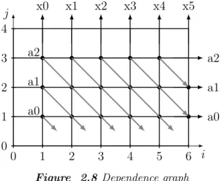
Dependence Graph

Dependence graph (DG) representation is used in systolic architecture design. The Fig. 2.8 0 1 2 3 4 5 6 i j 0 1 2 3 4 a0 a1 a2 x0 x1 x2 x3 x4 x5 a2 a1 a0

Figure 2.8 Dependence graph

represents the computation of the FIR filter:

y(n) =a0x(n) +a1x(n−1) +a2x(n−2).

The graph is regular and by using some linear mapping or projection techniques, sys-tolic architecture of the algorithm can be designed. Kung explained the motivation, advantages, and the basic principle of systolic architecture in [12].

In later chapters, the algorithmic representation is coarse-grain DFG. Each node does much more than simple addition or multiplication.

(19)

13

3. LIDE AND DICE

In the preparation of this thesis work, one integrated environment called DICE, was used to expedite the process of prototyping the Harris algorithm. The framework, LIDE, in which the algorithm was prototyped, is for modeling DSPs in software or hardware. This chapter provides introduction to both DICE and LIDE, and there will be some examples regarding how to use DICE.

3.1 The DSPCAD Lightweight Dataflow Environment

The DSPCAD Lightweight Dataflow Environment (LIDE), developed at University of Maryland, College Park, USA, is a flexible, lightweight design environment that allows designers to experiment with dataflow-based approaches for design and im-plementation of DSP systems [13]. LIDE comes with a set of predefined libraries, tools, and shell scripts. With LIDE, a designer can speedily develop a dataflow based DSP application.

In LIDE, a computation node (vertex) is called an actor. Edges for connecting actors are First-in-First-out (FIFOs). The design of actors is based on semantics of a dataflow model of computation called Enable-Invoke Dataflow (EIDF). In the preparation of this thesis work, we applied LIDE approach in C programming lan-guage and Verilog HDL. LIDE in C programming lanlan-guage is called LIDE-C, the framework in Verilog HDL is called LIDE-V.

The design of LIDE-C actors was inspired by object-oriented programming. Each actor has its construct, enable, invoke, andterminate function. Theconstruct func-tion is used for constructing an actor object, the funcfunc-tion initializes some values and assigns private members some values. Theenable function is a function, which detects the enable condition of an actor. An actor is only able to carry out compu-tation if it is enabled, i.e., the conditions for carrying out compucompu-tations are satisfied. The invoke function is the function, which carries out the actual computation. The

(20)

3.1. The DSPCAD Lightweight Dataflow Environment 14 terminate function is the deconstructor, it frees relevant memory space and does some "clean-up" tasks.

LIDE-V has main characteristics of LIDE, but it has hardware-unique features. For example, there is no construct and terminate functions in LIDE-V as there is no need to construct an object, let alone deconstruct it. LIDE-V is still being actively developed and tested, but LIDE-C is comparatively mature. To make things con-crete, we specially discuss LIDE-C in the following sections though the approaches discussed apply to other programming languages (MATLAB, CUDA, etc.). To pro-ceed, LIDE has to be installed before the following sections. The guide [14] provides information on how to install and set up LIDE.

3.1.1 Project Configuration

In C programming language, we need a Makefile besides the source programs to cre-ate an application. Without the use of integrcre-ated development environment (IDE), we probably need to create our own Makefile to conveniently build a project. In LIDE-C, we do not have the need to write Makefiles to compile programs. Instead we write a configuration file. A utility called dicelang-C is a package for building projects in LIDE-C. With dicelang-C package, we need to only write a Bash script called dlcconfig. The file contains project-specific files and some related variables. One example configuration file for Sobel edge detection project is shown in pro-gram 3.1

1 # !/ usr / bin / env b a s h

# S c r i p t to c o n f i g u r e t h i s p r o j e c t 3 # S o b e l e d g e d e t e c t i o n a l g o r i t h m d l c i n c l u d e p a t h =" - I . - I $ U X L I D E C / src / g e m s / c o m m o n \ 5 - I $ U X L I D E C / src / g e m s / b a s i c - I $ U X L I D E C / src / r u n t i m e " d l c m i s c f l a g s =" " 7 d l c m k l i b s =" " d l c t a r g e t f i l e =" $ L I D E C G E N / u s e r _ f u n c . a " 9 d l c i n s t a l l d i r =" $ L I D E C G E N " d l c o b j s =" S O B E L . o l i d e _ c _ s o b e l . o \ 11 l i d e _ c _ s o b e l _ s c h e d u l e r . o l i d e _ c _ u s e r _ f u n c t i o n . o " d l c v e r b o s e =" "

(21)

3.1. The DSPCAD Lightweight Dataflow Environment 15 The compiler that the package uses is the GCC compiler. Here we briefly explain the purpose of some variables in the script.

• dlcincludepath variable specifies predefined source code for compilation of our C project. LIDE-C FIFO definition and some other related modules are lo-cated in this path.

• dlctargetfileis the target file toward which we build. In this case, the target is a static library file and we will use it to build the final executable.

• dlcinstalldir is the installation directory where the target file is installed [13]. • dlcobjs is the variable which sets the names of object files.

More explanations on other variables are available in [13].

3.1.2 Project Build, Installation and Cleanup

Now the question we have is: how to build a project and how to install the ex-ecutable? To build a project, we need a Bash script called makeme. Here is an example makeme Program 3.2.

# !/ usr / bin / env b a s h

2 # S c r i p t to b u i l d t h i s p r o j e c t

4 s e t - a

source d l c m a k e m e

Program 3.2 An example makeme file

By running the script, we build our project easily. Installation takes no more than running a command called dlcinstall. dlcinstall will install the executable in the directory specified by the variable dlcinstalldir. For cleaning intermediate files, use a command called dlcclean is used.

3.1.3 Creating A Driver and Scheduler in LIDE-C

LIDE-C is used for implementing DSP dataflow graphs, the edges in dataflow graphs are modeled as FIFO. It is designer’s job to create actors, drivers, and schedulers.

(22)

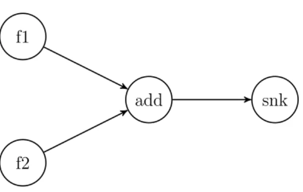
3.2. The DSPCAD Integrative Command Line Environment 16 A dataflow graph for implementing vector addition is shown in figure 3.1. To implement this graph in LIDE-C, we need to createfile sourcenodes like f1 and f2,

f1

f2

add snk

Figure 3.1 Vector addition graph

add, and snk. Besides, we need a driver where we instantiate all the actors and connections. For example, we decide the size of FIFOs and the datatype of it. In addition, all required actors should be constructed.

The execution of the whole graph requires a scheduler to schedule all the events in the graph. Depending on the application, we need different schedulers. LIDE-C comes with a library scheduler for execution of the whole graph. A smart scheduler can greatly improve efficiency of the graph, to that end we typically need to know some information about the system in advance.

3.2 The DSPCAD Integrative Command Line Environment

The DSPCAD Integrative Command Line Environment (DICE) [15] is a set of tools for easy use of LIDE. But DICE is a general tool for software development, the use of DICE makes it possible to develop software quickly and efficiently.

The important utilities, based on their niche use, under DICE can be classified as: directory navigation utility, copying and pasting utility, archiving and extracting utility, and unit testing utility. These utilities can be very handy and helpful when we deal with command line environment.

For directory navigation, DICE comes with main commands: g and dlk. The command g is short for go, if we pass a link name as argument to it, we will "go" to the directory the link points to. The command dlk is for creating a link, we can create a link name for a directory (path) with this command; Archiving and

(23)

3.2. The DSPCAD Integrative Command Line Environment 17 file extraction from a (e.g. tar) package becomes a lot easier with utilities such as

dxpack and dxunpack [15].

Unit testing is another great feature of DICE, the following section provides a brief introduction to the use of it.

3.2.1 Unit Testing

For software or hardware developers, a common task is to test if a design meets all the requirements. We want to feed some stimuli to our design and see the output from our design. If the design behaves the way we want, we are moderately confident that it is functioning the way it should.

DICE provides a utility calleddxtest for unit testing. The tool provides flexibility and language-agnostic features for testing. The implication is that: to use dxtest, there is no need to learn new syntax and that the testing framework can be used to test designs in different languages (Python, VHDL, Verilog, etc.).

To lauch a test on a directory, the directory must start with the word test. The following components are required for testing:

• README.txt file

The file provides some information about the test so that it is possible to work more in retrospect.

• A makeme file for building up project

The convention is the same for LIDE as discussed previously, themakemefile is similar to a Makefile in building up a project in other programming languages (e.g. C).

• A runmescript

The script is for running the driver and redirecting output to error output. • A correct-output.txtfile

As the name suggests, this file contains the expected output. • A file called expected-errors.txt

(24)

3.2. The DSPCAD Integrative Command Line Environment 18 With all of the above files ready, a test can be lauched by running dxtest com-mand. The utility compares the generated output with correct-output.txt and

(25)

19

4. LIDE-C IMPLEMENTATION OF HARRIS

ALGORITHM

This chapter focuses on LIDE-C implementation of the algorithm. The first step for building up an application in LIDE is high level modeling of the algorithm in MATLAB. High level modeling provides all the reference results for verification.

4.1 High Level Modeling

High level modeling is an important first step for building an application in LIDE-C, the purpose of it is to get all the reference results and give us a better grasp of how the algorithm works. MATLAB was chosen as the high level tool for modeling Harris algorithm. MATLAB is handy for such kind of modeling purpose as it has commonly used image operation functions available.

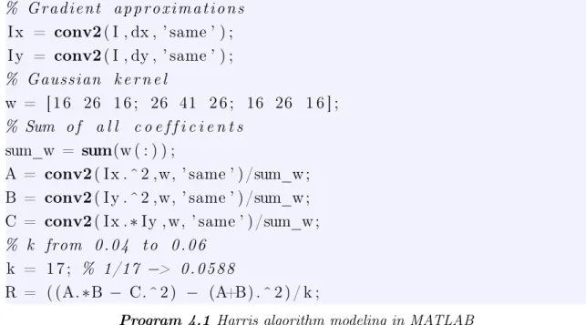
To have an idea on how the Harris corner detection algorithm works, the Program 4.1 gives us some insights about it. The lines for printing reference results are not shown in 4.1 due to space limit. The Program 4.1 shows only the operations which give us a general idea on how the algorithm works. For example, the preprocessing part is skipped. The variablesI,dx, anddyrefer to input image, horizontal kernel, and ver-tical kernel, respectively. The chunk of MATLAB code corresponds to three steps: gradient approximation, Gaussian smoothing, and calculation of the Harris measure.

(26)

4.2. Dataflow Graph of Harris Algorithm 20 % G r a d i e n t a p p r o x i m a t i o n s I x = conv2( I , dx , ’ same ’ ) ; I y = conv2( I , dy , ’ same ’ ) ; % Gaussian k e r n e l w = [ 1 6 26 1 6 ; 26 41 2 6 ; 16 26 1 6 ] ; % Sum o f a l l c o e f f i c i e n t s sum_w = sum(w ( : ) ) ;

A = conv2( I x . ^ 2 ,w, ’ same ’ ) /sum_w ; B = conv2( I y . ^ 2 ,w, ’ same ’ ) /sum_w ; C = conv2( I x .∗Iy , w, ’ same ’ ) /sum_w ; % k from 0 . 0 4 t o 0 . 0 6

k = 1 7 ; % 1/17 −> 0 . 0 5 8 8

R = ( (A.∗B − C. ^ 2 ) − (A+B) . ^ 2 ) / k ;

Program 4.1 Harris algorithm modeling in MATLAB

There are a few things to take note of in the MATLAB code. First, the test image is converted to gray image. Our purpose is to find corners and such change will not defeat our purpose. Second, Sobel kernel is used. The values of the variable dx can be set to anything, this means there is a possibility to experiment with different gradient approximation kernels. Indeed, different kernels were tested. Third, data representation is fixed-point representation. In this case, 32-bit fixed-point arith-metic is used, which, makes it possible to use integer aritharith-metic in C (LIDE-C). The MATLAB code is adjusted such that it is possible to implement an exact model in LIDE-C.

4.2 Dataflow Graph of Harris Algorithm

The MATLAB model can be straightforwardly expressed in the form of dataflow graph in Fig. 4.1:

in grd G har out

Figure 4.1 A DFG of Harris algorithm

The actors (nodes) in, out refer to input and output node respectively. The actor

(27)

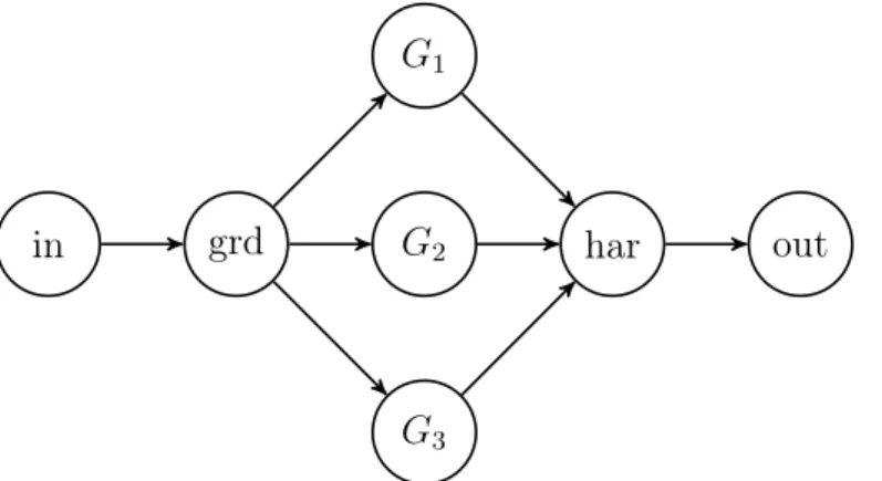
4.3. Details of Actor Design 21 smoothing. The actorharcombines the results, the output from this node is a Harris measure. The graph in Fig. 4.1 contains a lot of information, it is to some extent abstract. It does not specify anything about implementation details. A flattened graph which shows more details is shown in Fig. 4.2.

in grd

G1

G2

G3

har out

Figure 4.2 Flattened DFG of Harris algorithm

The flattened graph contains more nodes (actors) for Gaussian smoothing. The structure is intuitive considering that Gaussian smoothing is applied to three output channels. Different graphs for implementing the same functionality can be drawn for the application for different trade-offs. The computations in actors grdand G

involve image convolution as is discussed in chapter 2.

4.3 Details of Actor Design

With dataflow graph ready, the problem is how to implement the graph efficiently using LIDE-C. In LIDE-C, each actor has modes (mode) for carrying out compu-tation. An actor carries out different computation in different modes. Sometimes, one mode is used to initialize actual computation. To denote the transition between different modes, a mode transition graphcan be drawn [16]. In addition, a dataflow table can be made to illustrate the production and consumption rate of the ports of the actor [16]. The table should list all possible modes, ports, consumption (produc-tion) rate of an actor. The mode transition graph clearly shows the possible next mode from current mode. The dataflow table and mode transition graph are helpful for understanding properties and inner workings of an actor.

The Gaussian Actors

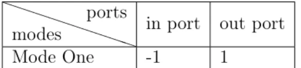
The dataflow Table 4.1 and mode transition graph of the Gaussian actors (G1,2,3

(28)

4.3. Details of Actor Design 22 P P_P P P P P P_P modes ports

in port out port

Mode One -1 1

Table 4.1 Dataflow table for Gaussian actors

These actors have the same structure and carry out similar computations, thus the dataflow table and mode transition graph are the same for them. The negative numbers in a dataflow table imply that the port consumes data in the mode, and positive numbers imply production. The values refer to the number of samples con-sumed or produced. One thing to take note of from the table is that the concon-sumed (produced) sample is a pointer. In our context, samples are not passed directly from one actor to another. Instead, pointers are passed between different actors. Passing a pointer between different actors saves a lot of traffic and allows for use of much smaller FIFOs. The mode transition graph is shown in Fig. 4.3. M1

M1

Figure 4.3 Mode transition graph of Gaussian actors

denotesMode One, as we can see from the figure there is only one legal transition. The key computation involved in Gaussian smoothing is window-based image con-volution. As discussed previously, the first step is to extract a window from the original image. After that, an element-wise matrix multiplication and summation is applied.

As pointers are used in computation, we need to figure out the addresses of all the elements that lie within a window. What makes things complicated is that there should be a mechanism to deal with corner cases, literally. The operation is regular most of the time, but what happens when the window is on the edge or on a corner. A mechanism called zero padding was used to deal with corner cases. The following Program 4.2 illustrates how extraction is done in C.

(29)

4.3. Details of Actor Design 23

1 i n t j = 0;

f o r( ; j < 9; j ++)

3 {

i f( m_s + j %3 >=0 && m_s + j %3 < s i z e && n_s + j /3 >=0 && n_s + j /3 < s i z e )

5 t e m p _ a r r a y [ j ] = i n p u t [ s i z e *( n_s + j /3) + m_s + j %3] ;

e l s e

7 t e m p _ a r r a y [ j ] = 0;

}

Program 4.2 Window extraction in C

The definitions of some variables are not displayed in the Program 4.2. The vari-ablesm_sandn_s refer to starting position where extraction starts. The variable temp_array is the array for storing the extracted matrix. The size variable in the code refers to image size, the number of columns (rows). Depending on the size of kernel, if 5 by 5 kernel was used the number of iterations would be 25. Correspondingly, the number used for modulo and division operation should be 5. The extracted matrix is stored in an array called temp_array, and then matrix multiplication and addition are carried out. A function called matrix_mul was implemented in C for such purpose is shown in Program 4.3.

l i d e _ c _ o p e r a t i n g _ d a t a _ t y p e m a t r i x _ m u l ( l i d e _ c _ o p e r a t i n g _ d a t a _ t y p e * matrix , l i d e _ c _ o p e r a t i n g _ d a t a _ t y p e * ker , i n t s i z e ) 2 { i n t i = 0; 4 i n t sum = 0; l i d e _ c _ o p e r a t i n g _ d a t a _ t y p e * m ; 6 l i d e _ c _ o p e r a t i n g _ d a t a _ t y p e * k ; m = m a t r i x ; 8 k = ker ; // D e r e f e r e n c e p o i n t e r s t h en m u l t i p l y 10 f o r ( ; i < s i z e ; i ++) { 12 sum += (* m ) *(* k ) ; m ++; 14 k ++; } 16 return sum ; }

(30)

4.3. Details of Actor Design 24

The Gradient Approximation Actor

The actor grd in Fig. 4.2 is used for gradient approximation calculation. The design of the actor is very similar to those Gaussian smoothing actors. The input comes from only one channel and output goes to three channels. A dataflow table which specifies the consumption (production) rate of the actor is shown in Table 4.2. P P P P P P P P_P modes ports

in port out port 1 out port 2 out port 3

Mode One -1 1 1 1

Table 4.2 Dataflow table of gradient approximation actor

The computation the actor carries out is basically image convolution, the mode transition graph is the same as Fig. 4.3. As stated previously, Sobel kernel is used for derivative approximation. For use of different kernels, modification has to be done statically before compilation. In C 4.4, two one dimensional arrays are used to represent Sobel kernels.

1 l i d e _ c _ o p e r a t i n g _ d a t a _ t y p e Gx [9] = { -1 , 0 , 1 , -2 , 0 , 2 , -1 ,

0 , 1};

l i d e _ c _ o p e r a t i n g _ d a t a _ t y p e Gy [9] = { -1 , -2 , -1 , 0 , 0 , 0 , 1 , 2 , 1};

Program 4.4 Sobel kernel as one dimensional arrays

Harris Response Actor

Thehar actor in Fig. 4.2 is the Harris response actor. This actor combines results from three channels and produce a Harris response output. The computation can be formulated as:

R= (A∗B−C2)−k∗(A+B)2,

where A, B, and C refer to output from three channels of Gaussian actors. The parameter k is the Harris free parameter, and the value is usually between 0.04

and 0.06. The value R is the Harris response. In LIDE-C implementation, the arithmetic is in fixed-point. Instead of multiplying a floating point value, (A+B)2

is divided by 17 as 1/17approximates0.0588which is within the range of classical values of Harris free parameter.

The mode transition graph of har actor is the same as the one in Fig. 4.3. The dataflow table is shown in Table 4.3.

(31)

4.4. Optimizations 25 P P_P P P P P P_P modes ports

in port 1 in port 2 in port 3 out port

Mode One -1 -1 -1 1

Table 4.3 Dataflow table of combiner actor

In addition to computation, the actor has to deal with overflow. The problem can be circumvented by using double precision variable for storing intermediate results. But the fixed-point arithmetic imposes the constraint that only integers should be used. A dynamic range analysis showed that the maximum (minimum) value of intermediate result was beyond the representable range of 32-bit integers but within the range of 64-bit integer in C. The temporary variables, namely A,B,C, and R, which are used for storing intermediate results are of typelong long in C. Interestingly, the outputRcan still be larger than maximum positive (or minimum negative integer). Threshold values for quantizing overflown values are needed, in our case the threshold values were2147483647 and −2147483648.

The final Harris response is a 32-bit integer, converting fromlong long type toint

type in C has to be done with caution. Explicit conversion is required for error-free operation.

4.4 Optimizations

One optimization related to LIDE-C dataflow graph implementation is passing pointers in FIFOs. In general, samples are passed inside FIFOs and in this case if we pass actual image arrays inside FIFOs, there will be a huge memory space required for each FIFO, let alone the overhead of copying data between FIFOs and actors. By passing pointers around, the requirement for large FIFO is removed, a FIFO’s size can be just one. This optimization decreases memory space and im-proves processing speed.

Another optimization is using static scheduling. Scheduling the execution of different actors can be challenging. The basic philosophy which was used was: the firing of upstream actors ensure the firability of downstream actors. This way, there is no need for dynamical checking of execution completion of upstream actors or firing condition check. The execution time will be shorter in this way.

(32)

26

5. LIDE-V IMPLEMENTATIONS OF HARRIS

ALGORITHM

LIDE environment is for prototyping DSPs swiftly, the framework in Verilog HDL is called LIDE-V. This chapter provides a brief introduction to inter-actor connections in LIDE-V, and different implementations of Harris algorithm in it.

5.1 Actor Level Interconnections

In software implementations of LIDE, actor related functions are implemented as member functions of the actor. In LIDE-V, the computations are mapped on hard-ware units. Besides, in hardhard-ware there are no concepts as constructors and destruc-tors. Once an actor is instantiated, it is there "forever". The implication is that a high level of parallelism.

The important modules at actor level areenable,invoke, and schedulermodules. A graphical representation (assuming distributed scheduling, which is true in our case) which illustrates the connections between different modules is shown in Fig. 5.1. The enable module, whose functionality is similar to LIDE-C enable module, checks the firing conditions of actors. When firing conditions are satisfied, the out-put signal called enable, will be set "high". The input signals of this module are population of input FIFOs, free space of output FIFOs, and the mode in which the actor operates. The module can be timed or untimed, meaning it can be imple-mented using combinatorial circuit or sequential circuit. The enable modules we used were implemented using combinatorial logic.

The invoke module is the module where computation is actually done, there is an input signal calledinvoketo this module, and computation starts wheninvokeis set "high" for a clock period. The computation completion is flagged by a signal called

fc (denoting "firing complete"), and the signal remains "high" when computation is done. The two signals are used for communicating with scheduler module which

(33)

5.2. Enable Block 27 will be described below; Reading input data and writing output data are done by "enable" hand-shaking mechanism. The scheduler module is for scheduling computation events. It tells the mode in which actors operate, and set invoke signal "high". Usually, it is up to the actor itself to decide the mode in which it operates. But the behaviour can be overridden by the scheduler, the implication is that usually scheduler does not need to drive the mode output signal.

FIFO FIFO invoke enable scheduler invoke mode_in enable mode_in fspace wr_en d_out fc next_mode rd_en pop_in d_in

Figure 5.1 Actor-level interconnections

5.2 Enable Block

In this section, our focus is on combinatorial Enable module. As an example, an Enable module for an actor with just one input channel and one output channel is shown in Fig. 5.2.

The Enable block in Fig. 5.2 checks that there is at least one sample in the input FIFO and at least one free slot in the output FIFO. Although it is an example for a simple case, the Enable module can be easily extended to actors with more input and output channels. There is very little modification required, that is why, as we will see soon, we can have code generation mechanism to take care of that.

(34)

5.3. Scheduler Block 28

Figure 5.2 Enable module RTL schematic

5.3 Scheduler Block

Scheduler block is the controlling center for actors. It decides when an actor can fire, schedulers can be centralized or distributed. In our case, for better performance of the algorithm, distributed schedulers are used. This means each actor in a dataflow graph has a dedicated scheduler. The Fig. 5.3 shows the RTL schematic of a generic scheduler. Some signal names are displayed in the picture, on the left are the input

Figure 5.3 Scheduler module RTL schematic

signals. It should be noticed that this generic scheduler does not interfere with mode transition (as the next_mode_in signal is connected directly to next_mode_out signal).

5.4 Capitalizing on the Regularity

LIDE-V is a regular Verilog framework as it complies with all the principles of LIDE, the regularity implies advantages when it comes to modeling DSPs in it. Each actor

(35)

5.4. Capitalizing on the Regularity 29 in LIDE-V works in a similar fashion, i.e., Enable-Invoke Dataflow. Capitalizing on the regularity improves the efficiency with which we prototype DSPs in Verilog HDL. To that end, a script called gen_actor.py was created to generate actor-related modules and testbenches. The script is able to generateenable,invoke,scheduler, and wrap modules. The wrap module is a module which wraps aforementioned three modules. In addition, a testbench module for verifying the functionality of the actor can be generated in the form of SystemVerilog.

The ability to generate testbench in SystemVerilog is crucial as verifying is usually the most time-consuming part in hardware design. The use of SystemVerilog means that we can exploit advantages of the language more compared to primitive Verilog. The other generated modules are in the form of primitive Verilog form, which, is exactly what we want as LIDE-V imposes such constraint. The functionality of each Verilog module is, depends on the context, naturally up to the designer to fill in. One of the principles of LIDE-V is to create efficient hardware "infrastructure" for implementing abstract, complicated systems.

The testbench module requires minimum modification from the designer. What the designers need to do is adding application-specific parameters. Adding parameters cannot be done by code-generation mechanism as application-specific assumption, like the parameters used, cannot be made. But fill in a few parameters in the generated testbench is a trivial and error-free operation.

5.4.1 Code Generator

The idea of using some sort of code generation mechanism does not seem to be consistent with LIDE-V’s principles. LIDE-V is not high level synthesis (HLS) and the designer should take care of low level details of the designs. Under scrutiny, code generation here is a means of expediting developing process. The generated code will not be inferred to logic in hardware, and it is up to the designer to decide how to code an algorithm.

The fundamental idea of the code generator can be summarized as "smart printing". Printing is often used in programming for the purpose of debugging, and in my case it is about printing (writing) programs to files. Simply put, code generator is a program which, by capitalizing on the regularity of LIDE-V framework, can write programs; The code generator was implemented in Python. Python was chosen

(36)

5.4. Capitalizing on the Regularity 30 because of its expressiveness, support for different programming paradigms, and very powerful libraries. The Python code generator can be divided into two parts: the command line parser part and the generating part.

Command Line Parsing

Parsing is relatively simple, the generator accepts three arguments and they are actor name, the number of input channels and the number of output channels. If there are not enough arguments fed to the generator, the program exits showing an example use of it. This is done by using argv fromsys library in Python.

The following step in parsing is to check the number of input/output channels. Apparently, numbers should be passed as arguments. The additional requirement is that the number of channels should be at least one. In Python code, there is a function called check_legal_size() which is dedicated for checking legal number of input/output channels.

Generating Code

When parsing is done, next issue is actually code generation. One key function is called concat which accepts four arguments and prints some text to files based on input arguments. Basically, the function prints the specified certain number of times with or without comments. The rest of the generator code is about repetitive calling of the function.

The code for generating actor-related templates is very simple, but the part for generating actor’s testbench is relatively complicated. There are questions that need to be solved. How do we justify the correctness of the generated testbench? To deal with that problem, example testbench code for verifying simple addition actor was used as reference. Verifying steps are very similar across actors with different functionalities. The generated testbench fills the input FIFOs connecting the actor in a sequential fashion, meanwhile the testbench checks the population of output FIFOs in parallel. The input, however, is assumed to be from text files with binary strings in them. The output, on the other hand, is written to text files with binary strings in them also.

5.4.2 Usage of Code Generation Mechanism

The use of the script is very simple, the following line demonstrate the use of it. $python gen_actor . py <a c t o r−name> <i > <o>

(37)

5.5. Straightforward Implementation and Unfolding 31 In the above code, i refers to the number of input channels while o refers to the number of output channels. Theactor-namefield is for generating actor templates and testbench of that name. To make things concrete, suppose we need to create an actor called Gauss for Gaussian smoothing, and the actor has 3 input channels and 1 output channel. To generate this actor’s templates and testbench, we can use the following command:

$python gen_actor . py Gauss 3 1

Four actor related files will be generated, they areGauss_invoke.v,Gauss_enable.v

Gauss_control.v, Gauss_wrap.v and one testbench file calledtb_Gauss.sv.

5.5 Straightforward Implementation and Unfolding

Implementing a dataflow graph which straightforwardly describes the computations is relatively easy. The first implementation we had was based on the dataflow graph in Fig. 5.4. The graph is not too much different from what is shown in the previous

in grd

G1

G2

G3

har nom out

Figure 5.4 Straightforward Implementation of Graph

chapter, here one more actor called nom, used for non-max suppression, is added. The following text of this section will focus on describing the actors in this graph. We start from upstream actors to downstream actors.

5.5.1 Design of Gradient Approximation Actor

The gradient approximation actor is marked as grd in the dataflow graph in Fig. 5.4. Since the actor uses Sobel kernels for gradient approximation, there is an

(38)

5.5. Straightforward Implementation and Unfolding 32 internal memory space for storing a 3by3 matrix. This 3by3 matrix is for saving extracted window from the input image, and the matrix is then used for carrying out computing derivatives of two directions.

This actor has three modes of operation, they are WU, RE, and WR, representing WARM-UP, READ, and WRITE respectively. A mode transition graph for illus-trating the operations of the actor is shown in Fig. 5.5. The WU mode is for

WU RE WR

Figure 5.5 Mode transition graph for grd actor

warming up the system, namely, fill the pipeline with samples. After that, the actor mode switches between RE and WR. A dataflow table for explaining consumption and production rate is shown in Table 5.1.

P P P P P P P P_P modes ports

in out out out

WU -1 0 0 0

RE -1 0 0 0

WR 0 1 1 1

Table 5.1 Dataflow table for grd actor

The calculation of both (horizontal and vertical) derivatives takes no "time", two dedicated combinatorial circuits are used for calculating both derivatives.

5.5.2 Design of Gaussian Actors

The Gaussian actors which are shown in Fig. 5.4 are three instances of the same actor. These actors carry out Gaussian smoothing, and the kernel is of the following form: K =         1 4 6 4 1 4 16 24 16 4 6 24 36 24 6 4 16 24 16 4 1 4 6 4 1         .

(39)

5.5. Straightforward Implementation and Unfolding 33 The coefficients are hard-coded in a separate coefficient module, this way it is easy for synthesis tool to optimize. Gaussian smoothing is basically window-based image convolution, an important insight for window-based operation was derived from the paper [17] in which a primitive called ADL was proposed. ADL is short for Array Delay Line, it is used for extracting a window from images. The Fig. 5.6 illustrates how it works. Initially, there is nothing in the array of registers. The first sample

image column

K

Figure 5.6 Array Delay Line illustration

fills the rightmost register on the bottom. When the next sample comes in, the first sample shifts left so there is space for the incoming sample. The direction in which elements move in the ADL is marked by dotted arrows. By the time the ADL is filled with samples, we also get the first window (as marked by a K by K thick-line square) of elements.

We only start extracting a window when the ADL is warmed up completely, after that when there is a new sample coming in the element on the leftmost corner will be shifted out and we have a new window of samples. This scheme makes window-based operation very easy. The rest of actors whose core operation involves window-based operation all use this ADL. For example, the nom actor, whose operation is also window-based, also uses ADL as its memory. The mode transition graph for the actor is the same as Fig. 5.5, and the dataflow table is similar to Table 5.1.

(40)

5.5. Straightforward Implementation and Unfolding 34

5.5.3 Design of Harris Response Actor and Non-Max

Sup-pression Actor

The Harris response actor, called har, carries out the following computation: R= (A.∗B−C∗C)−(A+B)∗(A+B)∗k,

whereA,B, and C are matrices,k refer to the Harris free parameter. It is relatively straightforward to implement the actor in LIDE-V as there is no involved operation other than addition and multiplication. This actor has only one mode in which it reads inputs, i.e., A, B, and C, and write to output FIFO. A dataflow table and mode transition graph are trivial in this case.

The non-max suppression actor, called nom, involves many comparisons. This ac-tor has only two modes: WU and NORM, representing WARM-UP and NORMAL mode respectively. After warm-up, the actor stays in NORM mode. The first imple-mentation we had was that the actor uses only one comparator for all comparisons. A complicated scheduling was used for that.

5.5.4 Unfolding

In the previous actors, we have seen actors, namely, G and nom involve a lot repeated operations like multiplication and comparison. In the straightforward im-plementation, the actors use only one multiplier or comparator. We can improve the throughput of the system by applying a design technique called unfolding [18]. The basic idea behind unfolding is throwing more hardware for computations. Pre-viously, only one multiplier and one comparator were used. What if we can use two, three or even more? The direct impact is that we get the final results a lot quicker. For the Gaussian actors, they carry out 5 by 5 image convolution. If we use 5 multipliers, we collect the final output after waiting for only 5 clock cycles. What if we use 25 multipliers? We collect the results after one clock cycle. The same holds true fornomactor, but unfolding for thenomactor will not increase FPGA resource usage to a great extent as comparison is relatively a "cheap" operation. In Fig. 5.4, if we combine actors of different unfolding level we get different implementations of the same graph.

(41)

5.6. Harris Algorithm with Inter-actor Resource Sharing 35

5.6 Harris Algorithm with Inter-actor Resource Sharing

The implementation of Harris algorithm in LIDE-V can vary a lot, even the same dataflow graph can be implemented differently when different tradeoffs are our design targets. Implementing a graph that uses a tiny amount of FPGA resource is often a goal in hardware design, the Harris algorithm graph in chapter 4 illustrates a straightforward way of implementing the algorithm. There is no resource sharing between different actors albeit the functionalities of actors overlap greatly.

Resources in the Harris graph mean both memory resource and functional unit, but in this section inter-actor resource sharing refers to sharing of functional units between different actors. The Gaussian actors carry out the same type of operation, the only difference is that they operate on different data; A different graph for resource sharing between different actors is shown in Fig. 5.7. The dataflow graph

in grd

G1

G2

G3

FU har nom out

Figure 5.7 Inter-actor Resource Sharing Dataflow Graph

looks different from the original one, not only that but also the functionalities of actors in this graph are a bit different. The actors that require a new design are Gaussian actors and Harris response actor, while the FU is a new actor.

5.6.1 Design of Gaussian Actors

Since Gaussian actors share the same functionality units, there are no functional units in Gaussian actors. These actors are just dummy actors which do not carry out actual computation. They have separate memory space for storing input samples, as described previously, Gaussian actors carry out window-based operations, these actors will output a window of pixels.

(42)

5.6. Harris Algorithm with Inter-actor Resource Sharing 36 A mode transition graph and dataflow table help to understand better how the actors operate. These actors have the same transition graph and dataflow table. The modes are explained below:

WU RE WR

Figure 5.8 Dummy Gaussian actor mode transition graph

WU: is warm-up mode. In this mode, the actor reads one sample. As we can see from the transition graph, the actor can either stay in this current mode or go to

RE mode next time it is invoked. Internally, there is a invocation counter which keeps track of the number of times is has been invoked.

RE: is short for READ mode in which it reads one input sample. The next mode will always be WRmode. This is because after warming up the system, every time only one new sample is required to extract a window.

WR: represents WRITE mode in which it writes one output sample. There is a counter to keep track of the number of pixels in a window that have been written. The dataflow table is shown in Table 5.2.

P_P P P P P P P_P modes ports

in port out port

WU -1 0

RE -1 0

WR 0 1

Table 5.2 Dataflow table for dummy Gaussian actors

The design of actors has to be done carefully and differently from LIDE-C actor design. In LIDE-C, the firing condition is usually when there are many samples in input FIFO or many free space slots in output FIFO. In LIDE-V, we should use a limited resources while maintaining high performance. The design philosophy of LIDE-C should not be used directly in LIDE-V. The above design technique were used throughout different LIDE-V graphs.

(43)

5.6. Harris Algorithm with Inter-actor Resource Sharing 37

5.6.2 Design of Functional Unit Actor

FUis short for functional unit, this is the actor where computation actually occurs. A good starting point to get to know how the actor operates is by looking at the mode transition Table 5.9. There are four modes for this actor, M1, M2, and M3 are

M1

WR

M2 M3

Figure 5.9 Mode transition graph for FU Actor

for Gaussian smoothing of each channel. The WR mode is for writing output.The mode transition graph is fairly complicated, because scheduling the use of functional units is done by separating acess into different modes.

There is a lot of logic used for implementation of such mode transition graph. One thing to take note of is that when the actor is in WR mode, the next mode will always be either M1, M2 or M3. The dataflow table for this actor is shown in Table 5.3. All the Gaussian actors share the same functional unit actor, and this actor

P P P P P P P P_P modes ports in 1 in 2 in 3 out 1 M1 -1 0 0 0 M2 0 -1 0 0 M3 0 0 -1 0 WR 0 0 0 1

Table 5.3 Functional unit actor dataflow table

has only one functional unit, namely multiplier. This design uses a tiny amount of FPGA resources. As we can see from the dataflow Table 5.3 the consumption or production in a certain mode is always 1, this means the size of input and output FIFOs can be as small as 1.

(44)

5.7. Verification, Synthesis and Result Analysis 38

5.6.3 Design of the Harris Response Actor

The Harris response actor has to be redesigned, as we can see from previous dataflow graph there is only one input channel for all three types of inputs. This actor has two modes: RE and WR, representing READ and WRITE respectively. It has the kind of mode transition graph as shown in Fig. 5.10. The Fig. 5.10 nicely illustrates

RE WR

Figure 5.10 Mode transition graph for the Harris actor in inter-actor resource-sharing scenario

how actor mode transitions from one to another. Initially, the actor is in RE mode, and stays in the same mode after one more read. Then it switches to WR mode in which it writes the output. The dataflow table is shown in Table 5.4. Similar to

P P P P P P P P_P modes ports in out RE -1 0 WR 0 1

Table 5.4 Mode transition graph for Harris response actor

the functional unit actor, this actor requires very small input and output FIFO size.

5.7 Verification, Synthesis and Result Analysis

A DUT without verification cannot be said to be designed correctly, there is no point in synthesizing if we can not guarantee the correctness of designs. After that, we can synthesize the designs and collect results. Finally, we can do a result analysis on what we get.

5.7.1 Verification

Our ultimate goal is to have all the designs synthesizable, an important step is to verify the functionality of DUT. As mentioned previously, testbenches are generated

(45)

5.7. Verification, Synthesis and Result Analysis 39 for verification and we only need to add some actor-specific parameters to the gen-erated testbenches. This operation is basically error-free. To verify all the modules conveniently, a Bash script is used. For example, to verify an actor called grd. Simply running the following command:

$ s grd

will simulate all the related modules of grd actor. The command s is short for simulate. What the script does is creating a DO macro file for MODELSIM and starting MODELSIM for simulation. Before running the script, we should provide stimuli in the form of binary string format as we see below:

0 0 0 0 0 0 0 0 1 0 1 0 0 0 0 1 0 1 0 0 0 0

. . .

The number of bits and the length depend on the input data width of the actor, and how many input samples we want to use to test the DUT.

If there was no syntax error in the DUTs, there will be some generated files whose form is also in binary string. By using command diff to compare the generated output and expected we can decide if we should go back debugging or ensured that we have a correct design.

The verification of every single actor has gone through the same process, i.e., pro-viding stimuli, running simulation script, checking a match by using diff command.

5.7.2 Synthesis

To make synthesis easier, a script called rtl was created to expedite the process. The script uses sed to create a configuration file for XILINX Vivado and launches Vivado for synthesizing. Example usage of the script is shown here:

$ r t l g r d _ e n a b l e . v g r d _ c o n t r o l l e r . v grd_invoke . v grd_wrap . v

Or we can use the following: $ r t l grd∗. v

Image Processing Using Dataflow Techniques

JINGUI LI