Developing Land Management Units using Geospatial Technologies:
an Agricultural Application
Georgina Margaret Rose Warren
"This thesis is presented as part of the requirements for the award of the Degree of Doctor of Philosophy
of the
Curtin University of Technology"
To the best of my knowledge and belief this thesis contains no material previously published by any other person except where due acknowledgement has been made.
This thesis contains no material which has been accepted for the award of any other degree or diploma in any university.
Signature: ………
ABSTRACT
This research develops a methodology for determining farm scale land management units (LMUs) using soil sampling data, high resolution digital multi-spectral imagery (DMSI) and a digital elevation model (DEM). The LMUs are zones within a paddock suitable for precision agriculture which are managed according to their productive capabilities. Soil sampling and analysis are crucial in depicting landscape characteristics, but costly. Data based on DMSI and DEM is available cheaply and at high resolution.
The design and implementation of a two-stage methodology using a spatially weighted multivariate classification, for delineating LMUs is described. Utilising data on physical and chemical soil properties collected at 250 sampling locations within a 1780ha farm in Western Australia, the methodology initially classifies sampling points into LMUs based on a spatially weighted similarity matrix. The second stage delineates higher resolution LMU boundaries using DMSI and topographic variables derived from a DEM on a 10m grid across the study area. The method groups sample points and pixels with respect to their characteristics and their spatial relationships, thus forming contiguous, homogenous LMUs that can be adopted in precision agricultural applications. The methodology combines readily available and relatively cheap high resolution data sets with soil properties sampled at low resolution. This minimises cost while still forming LMUs at high resolution.
The allocation of pixels to LMUs based on their DMSI and topographic variables has been verified. Yield differences between the LMUs have also been analysed. The results indicate the potential of the approach for precision agriculture and the importance of continued research in this area.
ACKNOWLEDGEMENTS
There are many people who have assisted in the completion of this thesis and I would like to take this opportunity to acknowledge them. For those I have not mentioned by name, I say thank you, and acknowledge their valuable contribution of advice, support or material assistance.
Firstly I express sincere gratitude to my supervisor Professor Graciela Metternicht for her constant support, constructive comments and editing. Her expertise in remote sensing for agricultural applications provided extensive knowledge and guidance throughout this project. I am indebted to my associate supervisor, Jane Speijers, without her assistance in statistical applications this thesis would not have been possible. Jane was also involved in the painstaking editing process. My associate supervisor Professor Murray McGregor was involved in initial thesis discussions.
Without funding this research would not have been possible, as such I would like to thank the Department of Spatial Sciences at Curtin University of Technology for the initial stipend (Christopher Worth Memorial Scholarship) along with ongoing support from the CPSTOF project funded by a grant from the Australian Academy of Sciences, within the ARC-Linkage program (LP0219752) and its partners; The Department of Agriculture and Food Western Australia and SpecTerra Services. An Australian Postgraduate Award provided the majority of the funding throughout the thesis.
Field data collection has been a large part of this research and I would like to thank those involved for organising The Muresk Institute of Agriculture as a suitable location. Many people have assisted in the collection process they include; Gregor Brockmann who spent several weeks soil sampling, others that assisted were Mandy Jodrell and Tony Warren. For vegetation sampling Tammi Short and Bernhard Klingseisen assisted in the field and laboratory. Several months were spent at the Chemistry Centre WA performing chemical analysis on the soil. I would like to thank Dr Dave Allen and his team; Jeremy Brown, Jenny Harbord, Simon Adams and Katrina Walton for all their help.
Several organisations have shared either their data or resources and I would like to record my appreciation. These include; The Department of Agriculture and Food Western Australia, SpecTerra Services Pty Ltd, Muresk Institute of Agriculture and The Chemistry Centre of WA.
Numerous members of the Department of Agriculture and Food Western Australia have provided valuable assistance in differing ways; Buddy Wheaton, Henry Smolinski, James Fisher, Bill Bowden and Paul Galloway.
I would like to thank several colleagues within the Department of Spatial Sciences for their assistance and valuable lively discussions; Deavi Purnomo, Dr Zahurul Islam, Dr Rachael O’Brien, Todd Robinson, Bernhard Klingseisen, Dr Lesley Arnold and Lori Patterson. In particular Todd Robinson interpolated all the yield data, Bernhard Klingseisen developed LANDFORM while Dr Lesley Arnold and Lori Patterson assisted immensely with editing. I also thank Lisa Warren for her valuable time in editing and Des Thornton for all his tips and tricks in formatting the final manuscript.
Finally I would like to thank my family and close friends for their support during the entire research period. In particular the final 1½ years have been the most challenging in terms of combining being a new mum and research. Many thanks to those who have taken care of Isabella (especially her Gran) so I could work. Without your help, I wonder if this thesis would have ever been finished. To my wonderful husband Tony and gorgeous Isabella, it has all been worth it!
TABLE OF CONTENTS ABSTRACT... i ACKNOWLEDGEMENTS ...ii TABLE OF CONTENTS... iv LIST OF FIGURES ... xi LIST OF TABLES ... xv
LIST OF ACRONYMS AND OTHER ABBREVIATIONS ...xviii
CHAPTER 1 INTRODUCTION ... 1
1. 1 Problem Formulation ... 1
1. 2 Background ... 2
1. 3 Research Objectives... 3
1.3.1 Aims of the Research ... 3
1.3.2 Expected Outcomes... 5
1.3.3 Significance and Benefits of the Research... 5
1.3.4 Research Methodology ... 5
1. 4 Overview of Thesis ... 7
CHAPTER 2 LITERATURE REVIEW ... 10
2. 1 The Generation of Land Management Units... 10
2.1.1 Methods of Classification of Spatial Zones ... 12
2.1.1.1 Spatially Constrained Classification ... 20
2. 2 Landscape Attributes Required to Form LMUs... 22
2.2.1 Soil Properties ... 22
2.2.1.1 Soil Texture... 25
2.2.1.2 Coarse fragments... 26
2.2.1.3 Soil Stability... 27
2.2.1.4 Organic Matter ... 28
2.2.1.5 Cation Exchange Capacity ... 29
2.2.1.6 Soil Acidity ... 31
CHAPTER 2 continued
2.2.2 Vegetation ... 33
2.2.3 Topographic Attributes ... 34
2. 3 Methods for Recording Landscape Attributes ... 34
2.3.1 Field Sampling Techniques for Soil and Vegetation ... 34
2.3.1.1 Soil ... 34
2.3.1.2 Vegetation ... 39
2.3.2 Remote Sensing of Soil and Vegetation... 40
2.3.2.1 Reflectance of Vegetation... 41
2.3.2.2 Remote Sensing of Agricultural Crops ... 42
2.3.2.3 Selected Spectral Indexes for Agricultural Applications ... 46
2.3.2.4 Reflectance of Soil properties ... 48
2.3.3 Digitally Derived Topographic Attributes ... 54
2.3.3.1 Landforms ... 54
2.3.3.2 Compound Topographic Index ... 57
2.3.3.3 Slope... 59
2. 4 Validation Techniques for the LMU classification... 59
2.4.1 Comparisons with Yield Data ... 60
2.4.2 Spatial Map Comparisons ... 64
2. 5 Summary ... 67
CHAPTER 3 STUDY AREA AND DATA SETS ... 69
3. 1 Study Area... 69
3.1.1 Climate ... 70
3.1.1.1 Rainfall... 70
3.1.2 Soils... 73
3. 2 Remote Sensing Data ... 77
3.2.1 Calibration of DMSI ... 78
3.2.1.1 Select a Reference Image ... 79
3.2.1.2 Select Invariant Targets... 80
3.2.1.3 Calculate the Calibration Coefficients ... 83
3.2.1.4 Examine Calibration Curves and Adjust Targets... 83
CHAPTER 3 continued
3. 3 Digital Elevation Model... 88
3. 4 Yield Data ... 90
3. 5 Field Data... 93
3. 6 Software and Hardware... 94
3.6.1 Global Positioning System (GPS)... 94
3.6.2 GIS Software... 94
3.6.3 Statistical Software ... 94
3. 7 Summary ... 94
CHAPTER 4 FIELD DATA COLLECTION AND ANALYSIS... 96
4. 1 Soil Sampling Design... 96
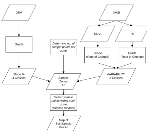
4.1.1 NDVI and RI Layers ... 98
4.1.2 Mask Layer ... 98
4.1.3 The Variability Map Layer... 99
4.1.4 Slope Class Map... 101
4.1.5 Variability Table ... 102
4.1.6 Slope Table ... 104
4.1.7 Sample Matrix... 105
4.1.8 Sample Zones and Sampling points ... 105
4. 2 Field Collection... 107
4. 3 Chemical Analysis of Soil Properties ... 108
4. 4 Building the Soil Database... 111
4. 5 Vegetation Sampling... 111
4. 6 Generation of Vegetation Indices... 115
4. 7 Relationship between DMSI and Crop Attributes ... 116
4. 8 Factors Affecting the Relationship between DMSI and Crop Attributes 117 4.8.1 Vegetation Indices and LAI ... 118
4.8.2 Wheat ... 121
4.8.3 Lupins... 122
4.8.4 Canola ... 123
4. 9 The Use of DMSI for Characterising Vegetation Variability ... 125
CHAPTER 4 continued
4. 11 Summary ... 126
CHAPTER 5 GENERATION OF TOPOGRAPHIC ATTRIBUTES AND ANCILLARY POINT DATA... 128
5. 1 Landform Classification... 128
5. 2 Implementation of Landform Classification ... 129
5.2.1 Comparison between Semi-automated and Manually Derived Landforms ... 132
5.2.2 Forming Landform Variables... 133
5. 3 Compound Topographic Index ... 136
5. 4 Implementation of CTI... 138
5. 5 Generation of a Slope Percentage Map... 141
5. 6 Extracting Ancillary Data at Soil Point Locations... 142
5.6.1 Extracting Topographic Attributes... 142
5.6.2 Extracting DMSI for Soil Points in Areas without Vegetation Cover 143 5.6.2.1 Selecting Locations with Minimum Vegetation Cover... 144
5. 7 Yield Data Sets... 145
5.7.1 Extraction of Interpolated Yield Values ... 146
5.7.2 Potential Yield Estimation at Sample Points (Yield Data Set 1) ... 148
5.7.2.1 Multiple Regression Analysis ... 148
5.7.2.2 Estimation of Potential Yield at Sample Point locations ... 150
5.7.3 Actual Yield Data at Soil Points for 2002 and 2003 (Yield Data Set 2) 151 5. 8 Extracting Ancillary Data for the Mask Area ... 152
5.8.1 Extracting Topographic and DMSI Variables on a 10m Grid ... 152
5. 9 Summary ... 153
CHAPTER 6 SELECTION OF VARIABLES FOR USE IN FORMING LAND MANAGEMENT UNITS... 155
CHAPTER 6 continued
6. 2 Selecting Variables Based on their Association with Crop Yield... 157
6.2.1 Transforming Variables ... 157
6.2.2 Correlation Analysis ... 159
6.2.3 Associations between Yield and Landforms... 160
6.2.4 Multiple Regression between Yield and Soil Properties... 161
6.2.5 Discussion of Results ... 163
6. 3 Selecting Variables Using Principal Component Analysis... 165
6. 4 Relationships between Selected Soil properties and ancillary data ... 173
6.4.1 Correlation Analysis ... 174
6.4.2 Analysis of Variance with Landforms ... 174
6. 5 Summary ... 176
CHAPTER 7 A FRAMEWORK FOR CREATING LAND MANAGEMENT UNITS ... 177
7. 1 The Land Management Unit Classification ... 177
7. 2 Part A: Forming LMUs from Soil Point Data... 180
7.2.1 Transforming Input Variables... 180
7.2.2 Estimating Geographical Parameters from Variograms ... 180
7.2.3 Determining the Scale and Form of Spatial Variation... 181
7.2.4 Forming the Similarity Matrix on Soil Variables ... 186
7.2.5 Determining the Geographic Distance between Sample Points... 187
7.2.6 Forming Matrix of Spatial Weights ... 188
7.2.7 Forming Principal Coordinates from a Similarity Matrix... 189
7.2.8 Selecting the Appropriate Number of LMUs... 190
7.2.9 Non-hierarchical Clustering of 250 Soil Points ... 194
7.2.10 Utilising Landform Variables ... 195
7.2.11 Analysis of Variance of Ancillary Data and LMUs... 195
7. 3 Part B: Further Defining LMU Boundaries using High Spatial Resolution Ancillary Data ... 196
7.3.1 Transforming Ancillary Variables ... 196
7.3.2 Similarity between Mask Pixels and LMUs; Option 1 ... 196 7.3.3 Discriminant Analysis between Mask Pixels and LMUs: Option 2 197
CHAPTER 7 continued
7.3.4 Forming the Geographically Weighted Dissimilarity Matrix between
Soil Based LMUs and Mask Data Set... 197
7. 4 Provisional LMUs ... 198
7. 5 The Land Management Unit Map and Unit Descriptions... 201
7. 6 Summary ... 208
CHAPTER 8 VALIDATION OF LMU CLASSIFICATION ... 210
8. 1 Choosing a Validation Procedure... 210
8. 2 Validation of LMU Allocation using Ancillary Data ... 211
8.2.1 The Random Selection ... 213
8.2.2 Part A: Forming LMUs based on Soil Point Properties... 213
8.2.3 Part B: Assigning Random Points to LMUs based on Ancillary Data 213 8.2.4 Part C: Assign Random Points to LMUs based on Soil Properties . 214 8. 3 Sensitivity Analysis of LMU Classification ... 216
8.3.1 Results from the Kappa Map Comparison... 218
8. 4 Relationship between LMUs and Yield ... 222
8. 5 Summary ... 224
CHAPTER 9 CONCLUSIONS AND RECOMMENDATIONS ... 225
9. 1 Conclusions... 225
9.1.1 Determine Stable Soil Properties that have the most influence on Yield Variability in the Agricultural belt of WA ... 225
9.1.2 Employ High Resolution, Readily Available, Cheap Ancillary Data Sets that are related to Soil Properties and/or Landscape Variability... 226
9.1.3 Develop a Methodology to combine information derived from High Resolution Data Sets and Soil Properties at Point Locations... 229
9.1.4 Produce a LMU Map with associated Soil Properties at Paddock Scale 229 9.1.5 Validate the Methodology for forming LMUs... 231
CHAPTER 9 continued
9.1.7 Determine the Opportunities and Limitations of using
High-Resolution Digital Multi-spectral Imagery as a diagnostic tool for monitoring
Crop Growth during the Growing Season... 232
9. 2 Recommendations... 233 9.2.1 Data Sources ... 233 9.2.2 Opportunities of DMSI ... 234 9.2.3 GIS Programming ... 234 9.2.4 Validations techniques ... 234 REFERENCES... 236 APPENDICES ... 259
A Daily rainfall 2002 and 2003... 260
B Soil Sampling Design... 263
C Drainage Classes ... 268
D Field Texture Estimation... 270
E Full Soil Database Schema ... 272
F Implementation of Landform Classification... 274
G Implementation of Compound Topographic Index... 277
H Slope Algorithm ... 280
I Significant Difference between Oats and Oaten Hay Crop Types ... 282
J Estimated Yield at Sample Points ... 284
K Soil Variables Transformations... 287
L Ancillary Variables Transformations ... 300
M Correlations between Soil Variables ... 304
N Regionalized Variable Theory ... 311
O Experimental Variograms ... 314
P Box-Plots of Soil Properties and Ancillary Variables ... 319
Q Results from Kappa Map Comparisons ... 323
LIST OF FIGURES
Figure 1.1 Flow diagram of thesis chapters ... 7
Figure 2.1 Spectral Partitioning of solar irradiance by vegetation... 41
Figure 2.2 Visible and near-infrared reflectance differences in vegetation due to senescence... 42
Figure 2.3 Soil reflectance spectra for a silt loam soil at varying moisture contents. Percentage of moisture content by weight shown above each curve ... 50
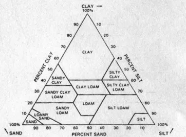
Figure 2.4 The textural triangle defines soil texture on the basis of sand, silt and clay ... 51
Figure 2.5 Example of a profile across terrain divided into morphological types of landform elements... 56
Figure 3.1 Study Area Location... 70
Figure 3.2 Rain gauge locations for Muresk Farm ... 71
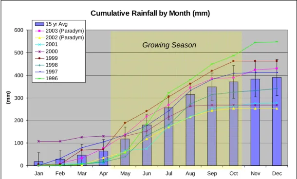
Figure 3.3 Cumulative rainfall by month for the years 1996 – 2003... 72
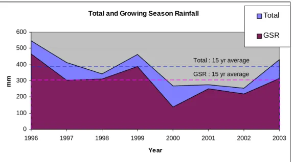
Figure 3.4 Total and Growing season rainfall for 1996-2003... 73
Figure 3.5 Muresk farm soils ... 75
Figure 3.6 Geographic distribution of target locations overlayed on reference image (DMSI June 2004)... 81
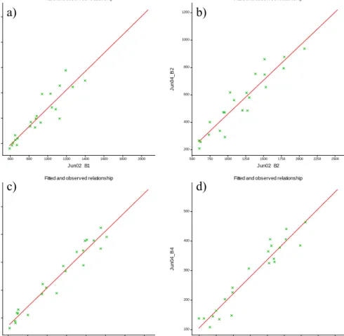
Figure 3.7 Scatter plots showing the least squares regression line for June 2002 imagery for a) Band 1, b) Band 2, c) Band 3 and d) Band 4... 84
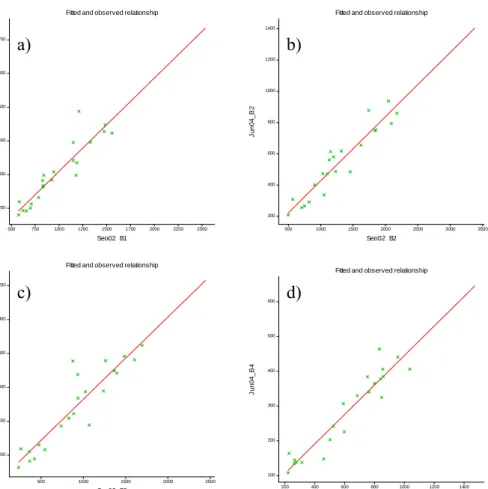
Figure 3.8 Scatter plots showing the least squares regression line for September 2002 imagery for a) Band 1, b) Band 2, c) Band 3 and d) Band 4 ... 85
Figure 3.9 Scatter plots showing the least squares regression line for September 2003 imagery for a) Band 1, b) Band 2, c) Band 3 and d) Band 4 ... 86
Figure 3.10 DEM systematic error in the form of tiling and a seam running north-south ... 89
Figure 3.11 An example of an interpolated yield surface overlayed with filtered yield points and paddock boundary... 91
Figure 3.12 Field data collection during June 2004 DMSI flight ... 93
Figure 4.1 Flow chart of sampling design... 98
Figure 4.2 Histogram of NDVI and RI change % values for mask region ... 100
Figure 4.3 Variability map generated with a 10m spatial resolution ... 101
Figure 4.5 Histogram of slope values for the area of interest ... 102
Figure 4.6 Spatial distribution of the soil sample points used for survey of the Muresk farm... 106
Figure 4.7 Soil sampling Field Data Collection... 107
Figure 4.8 Soil chemical analysis ... 109
Figure 4.9 Soil database schema ... 111
Figure 4.10 Field data collection and laboratory analysis... 114
Figure 4.11 Status of crops in year 2002 ... 119
Figure 4.12 Status of crops in year 2003 ... 119
Figure 4.13 Relationship between NDVI and Crops’ LAI ... 121
Figure 4.14 Spectral Curves for (a) 2002; (b) 2003... 124
Figure 5.1 Flow chart of implementation of Landform ... 129
Figure 5.2 Position of slope elements in a toposequence... 131
Figure 5.3 Map of landform classes across Muresk farm ... 132
Figure 5.4 Plot of principal coordinate scores ... 135
Figure 5.5 Upslope contributing area (A) is the area of land upslope of a length of contour (l). Specific catchment area (As) is A/l... 136
Figure 5.6 Flow chart of implementation of CTI in GeoMedia Grid... 139
Figure 5.7 CTI layer across Muresk Farm ... 140
Figure 5.8 Slope percentage map of the Muresk farm ... 141
Figure 5.9 Soil sampling points converted to 10m raster cells overlayed on landforms ... 143
Figure 5.10 Overview of process for extracting DMSI data at soil points with bare soil... 144
Figure 5.11 Soil sampling points with 3 x 3 neighbourhood window overlayed on a true colour DMSI composite... 146
Figure 5.12 Soil sampling points and their distance from field recorded GPS yield points overlayed on yield interpolated surface... 147
Figure 5.13 Plot of residuals against fitted values following Equation (5.5)... 149
Figure 5.14 Plot of residuals against fitted values for the final model ... 150
Figure 5.15 Frequency distribution of the Standardised Yield Estimations for the Soil Points ... 151
Figure 5.16 Frequency distribution of the yield 2002 at soil points ... 151
Figure 5.18 Overview of process for extracting DMSI data from 10m cells... 153 Figure 6.1 The relative amounts of water available and unavailable for plant growth
in soils with textures from sand to clay... 164 Figure 6.2 Biplots based on 250 soil points and the stable soil variables.
a) PC1 vs PC2; b) PC1 vs PC3 ... 167 Figure 6.3 Biplots based on 250 soil points and the stable soil variables.
a) PC1 vs PC4; b) PC1 vs PC5 ... 168 Figure 6.4 Relationship between pHw and pHca for 10 and 30cm depths ... 172 Figure 7.1 Flowchart of LMU classification... 179 Figure 7.2 Commonly used variogram models: (a) spherical; (b) exponential; and (c) Gaussian ... 183 Figure 7.3 Experimental and exponential model variograms for soil properties and
principal components after outliers have been removed... 185 Figure 7.4 Plot of a) g2S against g, b) Criterion S against g and c) logS against g
based on 13 soil variables ... 192 Figure 7.5 Plot of a) g2S against g, b) Criterion S against g and c) logS against g
based on 19 linearly independent soil variables... 193 Figure 7.6 Plot of a) g2L∗ against g, b) Criterion L∗ against g and c) logL ∗ against g
based on 13 soil variables ... 193 Figure 7.7 Plot of a) g2L∗ against g, b) Criterion L∗ against g and c) logL ∗ against g
based on 19 linearly independent soil variables... 193 Figure 7.8 Soil point LMU groups based on 250 soil points for a range of a) 200m, b) 250m and c) 300m ... 194 Figure 7.9 Nearest neighbour similarity assigned to a mask point for each LMU . 198 Figure 7.10 LMU groups based on Option 1: Cluster/Cluster analysis for a range of
a) 200m, b) 250m and c) 300m and Option 2; Discriminant analysis for a range of d) 200m, e) 250m and f) 300m ... 200 Figure 7.11 Biplot showing soil points within LMUs and canonical variate loadings
for CV1 vs CV2 ... 202 Figure 7.12 Biplot showing soil points within LMUs and canonical variate loadings
for CV1 vs CV3 ... 203 Figure 7.13 Biplot showing soil points within LMUs and canonical variate loadings
Figure 7.14 The Land Management Unit map for Muresk Farm... 206 Figure 8.1 Flowchart of random comparison/validation process... 212 Figure 8.2 Histogram of the percentage of correct assignment of S (50) random
points to LMUs for c (100) cycles ... 215
Figure 8.3 Kappa Map Comparison resultant agreement/disagreement maps for differing parameters a) Cluster/Cluster 200m b) Cluster/Cluster 300m c)
Discriminant 200m d) Discriminant 250m e) Discriminant 300m ... 219 Figure 9.1 (a) Muresk soil map versus (b) LMU map generated in this research. . 230
LIST OF TABLES
Table 2.1 Summary, in chronological order of methods for classifying spatial zones
... 14
Table 2.2 Texture grades based on clay content ... 26
Table 2.3 Determining the soil stability score for soils ... 28
Table 2.4 Ca:Mg ratio for USA soils ... 28
Table 2.5. Percentage of organic matter ratings at surface horizon (A1) ... 29
Table 2.6 Ratings for chemical properties ... 31
Table 2.7 Rating and salinity categories and associated effects ... 33
Table 2.8 Examples of Vegetation Indices ... 44
Table 2.9 Iron oxides and soil colour... 53
Table 2.10 Morphological type (topographic position) classes ... 56
Table 3.1 Description of Soil Survey hierarchy... 74
Table 3.2 Description of subsystem, landform and major soil types present in the study area ... 76
Table 3.3 DMSC Flight specifications... 77
Table 3.4 Dynamic range of pixel values for DMSI... 79
Table 3.5 Targets selected for calibrations ... 82
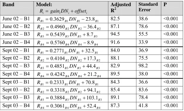
Table 3.6 Least-squares regression model for image calibration... 87
Table 3.7 Raw, Reference and Calibrated image statistics ... 88
Table 3.8 Interpolated yield data available for Muresk Farm... 92
Table 4.1 Definition of slope classes ... 97
Table 4.2 Change % range for variability class of NDVI and RI ... 100
Table 4.3 Initial and final selection of Pairwise Ratio Matrix values and Weights 104 Table 4.4 Variability proportion determination ... 104
Table 4.5 Number of sample points per slope class... 105
Table 4.6 Sample Matrix of slope and variability classes... 105
Table 4.7 Soil sampling field data collection... 108
Table 4.8 Methods of soil chemical analysis ... 110
Table 4.9 Transect Attributes... 112
Table 4.10 Methodology to determine crop density ... 113
Table 4.11 Basic descriptive statistics of crop attributes recorded on the transects115 Table 4.12 Correlation coefficient for crop LAI vs Vegetation Indices ... 117
Table 4.13 Correlation coefficient for canola PAI and LAI vs DMSI bands and LAI
vs Visual % Cover... 117
Table 5.1 Default values used for the generation of primary landforms ... 130
Table 5.2. The landform similarity matrix ... 134
Table 5.3. Percentage variance accounted for by 7 landform classes... 135
Table 5.4 Principal coordinate scores for landform PC’s ... 136
Table 5.5 Number of soil points with NDVI ≤0 ... 145
Table 5.6 A description of the two yield data sets and their attributes ... 146
Table 5.7 List of attributes recorded for soil and vegetation point locations during yield extraction... 147
Table 6.1 Stable soil properties and variables from literature review... 156
Table 6.2 Variable transformations and resultant skewness ... 158
Table 6.3 Correlation coefficients from analysis between yield and other variables ... 159
Table 6.4 ANOVA for Yield against Landforms... 161
Table 6.5 Regression results from analysis between yield and soil properties... 162
Table 6.6 Percentage of variance explained by each principal component and loadings of variables for each principal component from the 250 soil points . 166 Table 6.7 Correlation of texture and ECEC ... 169
Table 6.8 List of 13 soil variables to be included in LMU model ... 173
Table 6.9 Correlation between 13 selected soil properties and ancillary variables 174 Table 6.10 ANOVA for Soil Properties against Landforms ... 175
Table 7.1 Principal components of correlation matrix of 13 soil properties... 182
Table 7.2 Exponential variogram models for soil properties and principal components ... 184
Table 7.3 Percentage of variance accounted for by 13 PCO’s for effective ranges of 200m, 250m and 300m... 190
Table 7.4 Summary of principal coordinate analysis over several spatial ranges .. 190
Table 7.5 Significance of differences between LMUs formed at each range for ancillary variables ... 195
Table 7.6 Soil variables used in discriminate analysis... 201
Table 7.7 Percentage of variance explained and variable loadings of variables for each canonical variate ... 202
Table 7.9 Description of LMUs present in Figure 7.14 ... 207 Table 8.1 The contingency table in its generic form... 217 Table 8.2 The Kappa statistics; overall and for individual LMUs, used for
comparison with the LMU map based on a Cluster/Cluster method with a range of 250m ... 220 Table 8.3 Summary of the individual LMU group comparisons that have not been
mapped well (≥20 percent to another LMU) and LMU legend ranking... 221 Table 8.4 Accumulated analysis of variance for regression model in Equation (8.9)
... 223 Table 8.5 Predicted Yield for each LMU based on the regression model ... 223 Table 9.1 Stable soil properties and variables from literature review... 226 Table 9.2 Comparison of the cost of some high resolution data sets January 2007 227
LIST OF ACRONYMS AND OTHER ABBREVIATIONS
ANOVA Analysis of variance
CaMg Calcium/Magnesium ratio CTI Compound Topographic Index CV Canonical Variate
DEM Digital Elevation Model
dGPS Differential Global Positioning System DLI Department of Land Information DMSC Digital Multi-Spectral Camera DMSI Digital Multi-Spectral Imagery
DN Digital Number
ECEC Effective Cation Exchange Capacity ESP Exchangeable Sodium Percentage GIS Geographic Information System GPS Global Positioning System GSR Growing Season Rainfall LAI Leaf Area Index
LF_PC Landform Principal Coordinate LMU/LMUs Land Management Unit/Units MCK Map Comparison Kit
NDVI Normalised Difference Vegetation Index NDVIgreen Normalised Difference Vegetation Index-Green OrgC Organic Carbon
PA Precision Agriculture PAI Petal Area Index PCO Principal Coordinates PPR Plant Pigment Ratio
PVR Photosynthetic Vigour Ratio
RI Redness Index
SAVI Soil Adjusted Vegetation Index SSCM Site Specific Crop Management VI Vegetation Index/Indices WA West/Western Australia
CHAPTER 1 INTRODUCTION 1. 1 Problem Formulation
Precision Agriculture has been defined as ‘observation, impact assessment and timely strategic response to fine-scale variation in causative components of an agricultural production process’, and thus may cover a range of agricultural
enterprises, and can be applied to pre- and post-production aspects of agricultural enterprises (Australian Centre for Precision Agriculture, 2006). Site-specific crop management (SSCM) is one facet of precision agriculture and is defined as
‘matching resource application and agronomic practices with soil and crop requirements as they vary in space and time within a field’ (Whelan and McBratney,
2000). A cost effective and practical system of dividing a field into land management units that account for the spatial variability of crop production across spatially separable zones in Australia, needs to be offered for SSCM to be tested, accepted and adopted (Whelan et al., 2002a).
High resolution remote sensing imagery is useful for agricultural spatial planning at the farm scale, particularly when it is incorporated into a Geographic Information System (GIS) containing other secondary data sources such as terrain attributes. It offers farmers, farm advisors and extension officers, a system to identify areas within a paddock which can be managed differently based on their individual characteristics, and can be incorporated into various land use scenarios. Farmers have shown considerable interest in the opportunities presented by remote sensing, especially where its application can lead to improved farm management.
As with all new management tools, the new techniques require further investigation and economic justification before they are widely accepted and adopted by the farming community. This research addresses this requirement by developing a framework for determining land management units across an entire farm.
1. 2 Background
In Western Australia, current soil and land capability maps provide information suitable for studies at regional or catchment scale. However, such maps lack the level of detail required for sound planning at farm scale. John Blake (2001), the leader of the Western Australian Department of Agriculture and Food’s Precision Farming Group, stated that Precision Agriculture has the potential to manage variability in the State’s agricultural areas which probably have the most variable soils in the world (e.g. farms can have easily five changes of soil type in one circuit of the paddock) (Blake and Huffer, 2001).
Remote sensing imagery incorporated into a GIS has the potential to be useful in establishing the location and extent of soil variability. This is important as farmers have expressed the need for detailed assessment (at farm scale) of paddock conditions (e.g. soil and land capability maps adequate for decisions at farm scale) to aid in the planning of alternative land uses or land improvements according to the current conditions of the land (Blake and Huffer, 2001).
Dividing a paddock into relatively homogenous management units offers opportunities for the manager to exploit sites according to their specific capability. The delineation of land management units (LMUs), or zones, has been investigated using several techniques. They include a mechanistic simulation model based on detailed soil inventory and climate records (Alphen and Stoorvogel, 1998), multi-year yield estimates derived from Landsat Thematic Mapper imagery (Boydell and McBratney, 1999), multivariate K-means clustering utilising temporal yield data (Cupitt and Whelan, 2001; Dobermann et al., 2003; Whelan and McBratney, 2003),
continuous soil electrical conductivity (EC) measures (Nehmdahl and Greve, 2001), morphological and spectral filtering of elevation data and soil EC combined in binary form (Zhang and Taylor, 2001) and the classification of remotely sensed imagery using supervised and unsupervised methods (Yang and Anderson, 1996; Stewart and McBratney, 2001). These techniques have had differing levels of success. Approaches based on intensive sampling or continuous sensors to map crop yield and soil properties tend to be expensive and time consuming.
More cost effective techniques are clearly required in order to classify LMUs with the detail required for applications of precision agriculture. The methods based on cheap high resolution data sets in combination with soil properties recorded at point locations, which are investigated here, have the potential to minimise costs while still providing an output at the required level of detail. Sampling strategies for soil properties can take numerous forms (Burrough and McDonnell, 1998a; McBratney et al., 1999), and a strategy that addresses the variability of soil properties and
subsequently makes an optimal placement of sampling points can minimise cost. In this research, various strategies will be reviewed and an appropriate method implemented, which will result in a spatial database of soil properties for the case study area.
An analysis of high resolution data with soil properties and crop attributes will need to be conducted to determine their suitability for forming LMUs. Other high resolution data sets include Digital Multi-Spectral Imagery (DMSI) and terrain variables derived from a Digital Elevation Model (DEM). The uses of these data have shown some promise. For example several studies have highlighted relationships between terrain attributes and soil properties (Moore et al., 1993a;
Gessler et al., 1995; Boer et al., 1996; McKenzie and Ryan, 1999) while remotely
sensed imagery has been used in numerous vegetation studies (Weigand et al., 1991;
Cloutis et al., 1996; Mogensen et al., 1996; Cloutis et al., 1999; Metternicht et al.,
2000; Senay et al., 2000; Thenkabail et al., 2000; McNairn et al., 2002) and soil
based applications (Bowers and Hanks, 1965; Stoner and Baumgardner, 1981; Karmonova, 1982; Latz et al., 1984; Coleman and Montgomery, 1987; Escadafal,
1989; Henderson et al., 1989; Epema, 1993; Metternicht and Zinck, 1997). 1. 3 Research Objectives
1.3.1 Aims of the Research
The main objective of this research is to develop a framework for classifying a farm into paddock scale, homogenous land management units (LMUs) that can be linked
to the ‘patch zone management’ approaches used in Precision Agriculture. There are several principles upon which this framework has been based which should be understood by users before they adopt the methodology:
i. LMUs are based on stable soil properties;
ii. The scale of LMUs is finer than the minimum size of current paddocks; iii. The cost of producing the LMUs is kept low, so that the adoption by farmers’
advisory groups is facilitated, and;
iv. Data sets which are utilised are available in most agricultural regions of WA.
To satisfy these principles further aims of this research are to;
a) Determine stable soil properties that have the most influence on yield variability in the agricultural belt of WA;
b) Employ high resolution, readily available, cheap ancillary data that are related to soil properties and/or landscape variability;
c) Develop a methodology to combine information derived from high resolution data sets and soil properties at point locations;
d) Produce a LMU map with associated soil properties at paddock scale, and to; e) Validate the methodology for forming LMUs.
Addressing these aims encompasses the following steps;
• Collecting soil information (e.g. physical and chemical soil properties) and crop growth attributes across a selected study area;
• Investigating high resolution ancillary data that could be used in the formation of LMUs;
• Examining relationships between DMSI and crop growth variables to determine their use as diagnostic tools for depicting within paddock crop variability;
• Analysis of soil properties and yield data to determine soil properties that influence yield variability;
• Describing the relationship between LMUs and soil properties, and; • Examining the success of the LMU classification.
Further derivative aims have evolved which include;
f) To develop an effective field soil sampling strategy, and;
g) To determine the opportunities and limitations of using high-resolution digital multi-spectral imagery as a diagnostic tool for monitoring crop growth during the growing season.
1.3.2 Expected Outcomes The outcomes of the research are;
• A framework for rapid and efficient production of farm maps suitable for
decision making related to site-specific management within paddocks;
• A soil sampling strategy that reduces the amount and cost of field work and soil
laboratory analyses while still generating adequate information for producing LMUs and their associated soil characteristics, and;
• Spatial tools for explaining yield variability at farm and paddock level.
1.3.3 Significance and Benefits of the Research
The research will develop a framework for rapid mapping of LMUs that can be used by extension officers, farm advisors and farmers to make appropriate economic and environmental decisions on land uses, while limiting the cost of expensive sampling.
The LMUs will provide spatial zones that can be incorporated into automated land evaluation models and used to conduct land suitability analysis. Outputs that can be generated once the LMUs are defined and characterised include; physical suitability in terms of current use; proposed scenarios for improvements for paddock/sub-paddock level management, and; alternative land use scenarios.
An evaluation of the use of DMSI (flown by SpecTerra Systems) to support the generation of LMUs will provide potential users with the opportunity to assess whether it is an appropriate layer of information to be included in their farm management programs. It is anticipated that the findings will easily be adapted into the so-called “next generation” of satellites (e.g. Resource 21, IKONOS, Quickbird, OrbView-3) with similar spectral, spatial, and radiometric characteristics.
1.3.4 Research Methodology
The study comprises the following major components:
1) Review of relevant literature to determine techniques appropriate for LMU classification, stable soil properties and their relation to plant growth, suitable soil and vegetation sampling techniques, potential of remote sensing applications for detecting landscape variability, topographic attributes useful in soil/landscape studies and LMU classification validation techniques.
2) Process existing data sets, i.e. calibrate DMSI and interpolate yield point data to create a continuous surface.
3) Design and implement an optimal soil sampling strategy, and collect and analyse soil samples to form a comprehensive soil database.
4) Design and conduct vegetation sampling synchronous with capture of DMSI. Perform statistical analysis between in situ crop attributes and DMSI to
determine the potential of DMSI in detecting landscape variability.
5) Generate topographic attributes, namely landforms (utilising the LANDFORM system), compound topographic index (CTI) and slope percentage.
6) Conduct a statistical analysis between yield and soil properties, topographic attributes and DMSI to determine input data for LMU classification. Perform principal component analysis on soil properties to examine appropriate stable soil properties for the classification of LMUs.
7) Use a spatially weighted multivariate classification technique to form contiguous, homogenous LMUs.
8) Perform a validation process to assess the success of the LMU classification technique.
1. 4 Overview of Thesis
Figure 1.1 displays a flow diagram indicating the connection of each chapter contained within this thesis. The chapters’ components and their relationship to the thesis structure are detailed individually hereafter.
Chapter 1 describes the research problem, providing relevant background information and setting the research objectives.
Chapter 2 contains a literature review. It defines LMUs with a comprehensive review of methods for classification of the landscape into spatial zones, culminating in the selection of an appropriate methodology for this research. Stable soil properties are identified and described in relation to plant growth. These properties are used in the statistical analysis with yield data (Chapter 6). Methods of field sampling design and implementation for soil and vegetation are described, which will be implemented in the field data collection (Chapter 4). The fundamental relationship between remotely sensed imagery and soil and vegetation attributes are detailed highlighting the potential of high resolution remotely sensed data for characterising landscape variability. Topographic attributes that are related to soil and landscape variables are identified and described; and their generation is illustrated in Chapter 5. Chapter 2 concludes with a description of validation techniques which could be considered for the LMU classification.
The selected study area is described in relation to climate, current soil information and land use in Chapter 3. Existing data sets which include high resolution remote sensing data, digital elevation model, yield data and field data are detailed. Calibration of remote sensing data is included. The software and hardware used in the research are also detailed in Chapter 3.
Chapter 4 includes a detailed description of the soil sampling methodology and implementation. The resulting spatial soil database includes the soil properties to be statistically analysed in relation to yield data (Chapter 6) and selected as inputs into the LMU classification (Chapter 7). The collection of field vegetation attributes is detailed and a thorough analysis of their relation to DMSI is conducted.
The generation of topographic attributes namely; landform, compound topographic index (CTI) and slope derived from the DEM are explained in Chapter 5. These are statistically analysed to determine their appropriateness as inputs to the LMU classification in Chapter 6. Chapter 5 also includes the GIS process devised for extracting the yield, topographic and DMSI data at soil points. This method of
constructing the yield data sets is later used in the statistical analysis (Chapter 6). The procedure for extraction of the topographic and DMSI data for the remainder of the study area is also detailed.
The statistical analysis between yield data and soil properties, topographic attributes and DMSI data is implemented in Chapter 6 with the intention of determining the most influential properties on yield variability. These properties are subsequently used as the input to the LMU classification (Chapter 7). Correlation, multiple regression, analysis of variance and principal component analysis are performed.
The framework for developing LMUs is described and implemented in Chapter 7. A spatially weighted multivariate classification technique was selected as a consequence of reviewing relevant literature (Chapter 2). The classification has been conducted using several parameters and the most appropriate map of LMUs has been selected. The LMUs have been further described based on the soil properties and landscape attributes that would be appropriate to farmers and farm advisors.
A validation of the LMU classification is performed in Chapter 8. Three methods for determining the degree of success in the formation of LMUs have been used. Finally, conclusions and recommendations for future research are provided in Chapter 9.
CHAPTER 2
LITERATURE REVIEW
The purpose of this research, to “develop a framework for classifying LMUs” and the principles upon which the framework has been based , has been presented in the introductory chapter along with an overview of thesis structure. Chapter 2 continues with a relevant literature review.
The following literature review covers background information on several topics necessary in this research. Firstly, a review of methods used to classify spatial zones is included with emphasis on studies that would be useful at farm scale, incorporate multivariate data and produce homogenous zones. Compiled from the review of methods for generating LMUs, the most common landscape attributes used as inputs have been identified, namely soil properties, vegetation and topographic attributes. Subsequently, these attributes have been reviewed in relation to their effects on plant growth and/or use in landscape classification applications. Methods for the collection, measuring and/or derivation of the soil properties, vegetation and topographic attributes have been reviewed which range from field sampling, remote sensing through to digitally derived by means of the computation of existing data. Finally an overview of methods for validating the LMU classification approach has been included.
2. 1 The Generation of Land Management Units
As identified in Chapter 1, the main objective of this research is to develop a framework for classifying farms at paddock scale into homogeneous LMUs that can be linked to site-specific crop management approaches used in precision agriculture. The principals of the framework have been detailed, stipulating that the framework for forming LMUs should be (i) based on stable soil properties; (ii) at within paddock scale; (iii) affordable to farmers, and; (iv) utilise available data. The following section firstly identifies what a LMU is and then goes on to examine methods for their generation, summarising with an approach that will be used in this research.
Dividing a paddock into relatively homogenous LMUs offers opportunities for the manager to exploit sites according to their specific capability. LMUs have been defined by various authors, at various scales, for various purposes. Lloyd (2003) defines a LMU as “an area of land, with common soils and landforms that should be managed similarly, to maximise production and minimise land degradation”. Other
researchers have not used the actual term LMU, but management zones or units. Doerge (1998) defines a ‘management zone’ as “a portion of a field that expresses a homogeneous combination of yield-limiting factors for which a single rate of a specific crop input is appropriate.” And thus, to be successful, the factors included
in the delineation method must be based on the true causes that affect the crop yield at that site (Doerge, 1998). Lark et al. (2003) define a ‘management zone’ or ‘zone’
as “a region of a field defined according to some criteria on the assumption that all sites within a zone are expected to be subject to similar constraints on crop performance and, therefore, might be managed in the same way.” Although not
stating an actual definition, several researchers (van Alphen and Stoorvogel, 1998; Boydell and McBratney, 1999; Fleming et al., 1999; Whelan and McBratney, 2000;
Cupitt and Whelan, 2001; Stewart and McBratney, 2001; Whelan et al., 2002b;
Basnet et al., 2003) have described a management zone as being fairly homogeneous
in terms of yield (either being actual yield, potential yield, plant growth, growth conditions, or productivity). For this research, a LMU has been defined as “an area of land, similar in terms of the physical characteristics and production capabilities, which can be managed uniformly”.
To begin to identify a method and inputs used to classify LMUs, reviews of predictive methods of determining digital soil property maps (McBratney et al.,
2003; Scull et al., 2003) were consulted. These reviews have discussed the origin of
work by Jenny (1941), who defined five factors for soil formation, the model taking the mathematical form;
(
cl,o,r,p,t...)
f
S = (2.1)
where S is a soil property, cl represents climate, o stands for organisms, r relief, p
parent material and t time. Numerous surveyors have used this framework as a
method for understating the qualitative list of important factors in soil formation (McBratney et al., 2003). The general equation is somewhat difficult to solve, but
(McKenzie et al., 2000). Several researchers have adopted the model, holding
factors such as time and organisms constant (McKenzie et al., 2000; McBratney et al., 2003).
In the same vein, a LMU will be a function of influential factors and the LMU model will take the mathematical form;
(
x x x xn)
f
LMU = 1, 2, 3... (2.2)
where LMU is a land management unit, x1 to xn are input landscape attributes that can be recorded cheaply and have a dominating influence on within-paddock spatial variability of productivity. Importance not only lies in the x1 to xn factors, but the methodology utilised to combine the data layers to create meaningful, useable LMUs.
The following review collates several methodologies that have been applied for the delineation of fairly homogenous spatial zones within a landscape. These “spatial zones” have been derived for various purposes such as management zones, soil mapping, yield maps, salinity maps and vegetation classification to name a few, where the outputs are a homogenous class for the purpose of the investigation. The importance here lies with the methodology utilised to incorporate several spatial data layers to model the spatial zones.
2.1.1 Methods of Classification of Spatial Zones
In a review of approaches for making digital soil maps McBratney et al. (2003)
discuss several predictive methods, which include, linear models, generalised linear models (GLMs), generalised additive models (GAMs), tree models (classification and regression), neural networks, fuzzy systems, other methods (genetic algorithms, splines), strengthening models: bagging, boosting, expert (knowledge-based) systems, unsupervised classification and geostatistical methods. From the review of approximately 70 studies, McBratney et al. (2003) found that GLMs in the form of
multiple regression to be the most frequently used followed by co-kriging. While the use of regression trees and neural networks was not common.
O’Brien (2004) included a description and comparison of potential modelling approaches in search of an applicable method for tropical forage selection. The
models included logistic regression, GLMs and GAMs, artificial neural networks, classification and regression trees, environmental envelopes, fuzzy rule-based methods and Bayesian probability models. O’Brien (2004) details these approaches and highlights their strengths and weaknesses. To identify methods for classifying spatial zones further, Scull et al.(2003) in a review of predictive soil mapping,
classify the modelling methods into four main streams namely; geostatistical methods, statistical methods, decision tree analysis and expert systems.
The classification of the landscape into spatial zones has also been used widely in remote sensing applications. Jensen (1996b) discusses several image classification techniques which are characterised into four main approaches; supervised classification, unsupervised classification, fuzzy classification and methods that incorporate ancillary data in the classification process. The methods that incorporate ancillary data are of particular interest in this research, and they are further subdivided into a) geographical stratification in which ancillary data is used prior to classification to subdivide the image into strata, b) classifier operations, which incorporate ancillary data during the image classification process and c) post classification sorting, which further subdivides an image based on some set of rules after an initial classification has been done. A combination of these methods that incorporate ancillary data are d) layered classification and e) expert systems.
The reviews of McBratney et al. (2003), O’Brien (2004), Scull et al.(2003) and
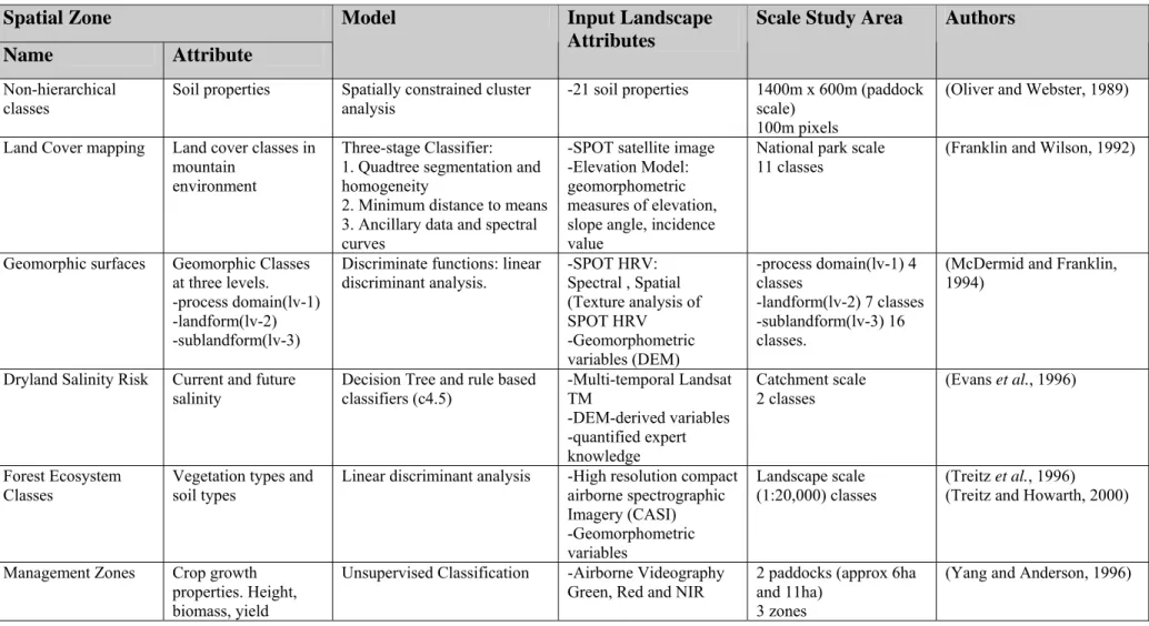
discussion of Jensen (1996b) have highlighted numerous approaches which could be considered in this research. However, there was not one methodology that could be identified from these reviews as the most promising for this research. Subsequently, studies that classify the landscape into spatial zones have been tabulated (Table 2.1) identifying their model/method used, input data and scale of study, to assist in pinpointing a method to be used to classify LMUs in this case.
Table 2.1 Summary, in chronological order of methods for classifying spatial zones
Spatial Zone
Name Attribute
Model Input Landscape
Attributes
Scale Study Area Authors
Non-hierarchical classes
Soil properties Spatially constrained cluster analysis
-21 soil properties 1400m x 600m (paddock scale)
100m pixels
(Oliver and Webster, 1989)
Land Cover mapping Land cover classes in mountain
environment
Three-stage Classifier: 1. Quadtree segmentation and homogeneity
2. Minimum distance to means 3. Ancillary data and spectral curves
-SPOT satellite image -Elevation Model: geomorphometric measures of elevation, slope angle, incidence value
National park scale
11 classes (Franklin and Wilson, 1992)
Geomorphic surfaces Geomorphic Classes at three levels. -process domain(lv-1) -landform(lv-2) -sublandform(lv-3)
Discriminate functions: linear
discriminant analysis. -SPOT HRV: Spectral , Spatial (Texture analysis of SPOT HRV -Geomorphometric variables (DEM) -process domain(lv-1) 4 classes -landform(lv-2) 7 classes -sublandform(lv-3) 16 classes.
(McDermid and Franklin, 1994)
Dryland Salinity Risk Current and future salinity
Decision Tree and rule based classifiers (c4.5) -Multi-temporal Landsat TM -DEM-derived variables -quantified expert knowledge Catchment scale 2 classes (Evans et al., 1996) Forest Ecosystem Classes
Vegetation types and soil types
Linear discriminant analysis -High resolution compact airborne spectrographic Imagery (CASI) -Geomorphometric variables Landscape scale (1:20,000) classes (Treitz et al., 1996)
(Treitz and Howarth, 2000)
Management Zones Crop growth properties. Height, biomass, yield
Unsupervised Classification -Airborne Videography Green, Red and NIR
2 paddocks (approx 6ha and 11ha)
3 zones
(Yang and Anderson, 1996)
Spatial Zone
Name Attribute
Model Input Landscape
Attributes
Scale Study Area Authors
Management Units Yield – indicating soil
variations Fuzzy Clustering -Multi-temporal yield data. 2-4 years 5 farms, 23 paddocks in total. (Mean paddock size 10ha)
2-7 zones
(Stafford et al., 1998)
Management Units Growth conditions Mechanistic simulation model -Detailed soil inventory (chemical and physical properties)
-climatic records
2 paddocks (10ha and 15ha)
13 zones
(van Alphen and Stoorvogel, 1998)
Management Zones Stable yield estimate
zones “FuzMe” Modified fuzzy k means -11 years Satellite based yield estimates “Farsite” based on Landsat TM acquired mid season
2 paddocks (each 182ha)
2 zones (Boydell and McBratney, 1999)
Management Zones Productivity Hand drawn vector lines -Soil colour aerial photography -topography -expert knowledge
1 paddock (71ha)
3 zones (Fleming et al., 1999)
Dryland Salinity Risk Predicted salinity risk (predicted discharge areas) and non-risk areas
Decision Tree Classifier (c5.0) -Multi-temporal Landsat TM
-DEM-derived variables -expert knowledge
Catchment scale
2 classes (Evans and Caccetta, 2000)
Land Cover Mapping Land cover classes Multi-step method.
1. Unsupervised classification. 2. Aggregation to raster polygons 3. Supervised, nonparametric classification 4. Optional postclassification sorting -Landsat TM image classification -DEM – topographic attributes 1700km2 12 classes (Wheatley et al., 2000) 15
Spatial Zone
Name Attribute
Model Input Landscape
Attributes
Scale Study Area Authors
Crop Management
Zones Significant differences in yield; differences in influential soil properties on yield
Multivariate k-mean clustering -Yield -3 years -Soil EC -Elevation data
1 paddock (100ha)
3 zones (Cupitt and Whelan, 2001)
Vegetation classes and subsequent bird abundance
Over and understorey
vegetation species Spatially constrained clustering -9 vegetation variables 45ha 50m pixels (Hall and Maruca, 2001) Management Zones Soil properties SEC continuous sensor
correlated with other soil properties
-Soil electrical
conductivity 1 paddock (10ha) 13 zones (Nehmdahl and Greve, 2001) Management Zones
(Contiguous) Soil properties Hard-k-zones algorithm -Yield – 3 years -Soil OC and K 1 paddock (17ha) 3 – 4 zones (Shatar and McBratney, 2001) Management Zones Yield potential 1. Maximum Likelyhood
classification on soil colour. i.e. soil type
2. Unsupervised
Classification using k-means clustering
-ETM+ of Landsat 7
30m pixels 2 paddocks (120ha and 150ha) 3 zones
(Stewart and McBratney, 2001)
Tropical forest
ecosystems Selvas
Spatially constrained cluster analysis
-Measures of vegetation activity from multi-temporal AVHRR imagery
-water balance variables modelled in GIS -elevation from DEM
Regional scale 8km resolution
(Mora and Iverson, 2002)
Management Zones Yield performance User-defined fuzzy set
membership function -Standardised Yield (4 years) 1 paddock (40.5ha) 3 zones (Basnet et al., 2003)
Spatial Zone
Name Attribute
Model Input Landscape
Attributes
Scale Study Area Authors
Yield zones Yield performance Ward’s clustering
k-means and fuzzy k-means clustering
-5 years of yield data 1 paddock (62.7ha) (Dobermann et al., 2003)
Management zones Yield response Combination of standardised
yield values -5 years of yield data 1 paddock (70.8ha) (Heermann et al., 2003) Management Zones Yield potential Multivariate K-means
clustering -2 x Yield -EC -Elevation data 1 paddock (75ha) 2 and 3 zones
(Whelan and McBratney, 2003)
Land Cover classes Managed grassland, woodland, rough grassland
Spatially weighted supervised classification; Method of incorporating spatial weighting into supervised classification
-Simulated remotely
sensed imagery Simulated 64 x 64 pixels (Atkinson, 2004)
Management classes Yield for potential
management Fuzzy k-means on 3 paddocks, then multiple discriminant analysis across farm
-Radiometric thorium, total counts, potassium, uranium
- Soil EC
- elevation, slope and CTI
3000ha farm
7 classes (Florin et al., 2005)
Management Zones Yield response
Nitrogen levels HERMES simulation 2 fields (20ha each) (Kersebaum et al., 2005) Soil property maps Soil attributes Linear regression
ordinary kriging plus regression
simple kriging incorporating ancillary data
-Soil properties: Texture, OM, pH, K -Bare soil aerial colour photograph. BGR wavebands
35m x 20m grid of 86 sample points (6ha)
(López-Granados et al.,
2005)
Spatial Zone
Name Attribute
Model Input Landscape
Attributes
Scale Study Area Authors
Management zones Soil or landscape conditions
Yield limiting factors
Fuzzy cluster analysis 3 approaches: a) relative elevation, organic matter, slope and EC
b) 6 years yield data c) relative elevation, organic matter, slope and EC, yield spatial trend, yield temporal stability.
2 fields:
32.8ha: 5 classes 12.5ha: 4 classes
(Miao et al., 2005)
Agricultural
Management Zones Soil properties and yield Cluster using filtering and fuzzy k-means -Elevation, slope, aspect, drainage area 1 field (9.8ha) 5 zones (Pilesjö et al., 2005) Management Units Soil-Landscape
features Spatially Constrained classification -Soil map. -relative elevation, slope -soil EC
-soil surface reflectance
52ha:
28 units merged to 6 units
(Simbahan and Dobermann, 2006)
Table 2.1 lists a literature review of classification methods for producing spatial zones highlighting their methodology, input factors and scale of study. As a summary of the works cited in Table 2.1, it can be observed that two thirds of the works are applied at paddock scale. The main focus of the review targeted paddock scale studies because the approach in this research will endeavour to provide LMUs that subdivide a paddock, however, in this case it will be implemented for the entire farm. As such, other catchment and regional scale applications have also been included to review methods and input data sets at those scales. The approach by Florin et al. (2005) is the only farm scale method, and they make the point that whole
farm applications remain elusive. Their approach uses a method that firstly forms zones on three paddocks and then allocates the classes across the entire farm.
Table 2.1 also shows that the four main input landscape attributes are soil properties, yield data, remote sensing data and topographic attributes. Soil properties have been used on more than one quarter of the techniques, almost all of which are paddock scale applications. Yield data have been used in approximately one quarter of the techniques, again all of which are paddock scale applications. Remote sensing data (recording vegetation attributes or soil properties) are used in half of the techniques, with over 50 percent of these being farm, catchment or regional scale applications. While topographic attributes are also used in almost half of the techniques with over 50 percent of these being farm, catchment or regional scale applications. It can also be summarised that all farm, catchment or regional scale applications used remote sensing and topographic attributes, which is not surprising as it is more common that such data are widely available at these scales as compared to more expensive point based data (i.e. soil properties).
Over one third of the methods included in Table 2.1 are either k-means clustering or fuzzy clustering (which is more often fuzzy k-means). Other more popular methods are spatially constrained clustering, decision tree classifiers and discriminant analysis. The k-means and fuzzy clustering methods are all used for paddock scale applications while spatially constrained clustering has been used at paddock and regional scales.
From the studies included in Table 2.1 the spatially constrained classification technique has a number of characteristics which make it the best method for this research. As for a number of methods, it can be used at paddock and regional scale and has the ability to incorporate multivariate data. The pivotal feature that makes it the best method listed is that it incorporates spatial relationships between objects into the classification, which group’s objects that are similar in terms of their attribute data. The resulting groups are spatially compact homogenous zones. While other methods can produce homogenous groups, they can be spatially scattered making them impractical for farm management. This problem is usually solved using post classification filters which inevitable introduce greater heterogeneity into the zones. The spatially constrained classification optimises the formation of zones with respect to both attribute homogeneity and spatial compactness, forming zones that can be practically managed by farmers. More details regarding the spatially constrained classification are discussed hereafter.
2.1.1.1 Spatially Constrained Classification
Similar to other classification techniques, spatially constrained multivariate classification (Urban, 2004) allocates samples to clusters based on their similarity with respect to measured variables (i.e. soil or terrain), but also considers their proximity to one another. This forces the clusters to be homogenous in terms of their variables, as well as, geographically contiguous (Urban, 2004). The technique is based on a similarity matrix of size n(n+1)/2 (n=number of sample points), which
becomes very large when classifying high resolution data sets (i.e. >100,000 individuals). Urban (2004) suggests that spatially constrained classification shows some promise, but is not yet computationally feasible for large datasets. In addition he mentions that while the classifications can yield patches that are better resolved spatially, they may be less well defined ecologically (i.e. on their measured variables). The use of spatially constrained classification will depend on the focus of the application. For example Caeiro et al (2003) applied three different classification approaches; (1) spatially constrained clustering followed by indicator kriging; (2) discriminant analysis; (3) a hybrid of 1 and 2, discriminant analysis with indicator kriging, and found method 1 that used the spatially constrained clustering to produce the more realistic pattern that was in better agreement with estuary behaviour (the measured variable).
There have been several differing procedures for incorporating the spatial weighting into the classification which are presented here. Legendre and Legendre (1998) offer a detailed description for spatially constraining a clustering methodology based on the similarity matrix, while Legendre (1987b) (cited in Legendre and Legendre, 1998) suggests weighting the values in an ecological similarity matrix by a function of geographic distance among sampling locations, prior to clustering. McIntire and Fortin (2006) used spatially constrained clustering which was constrained to only those plots that were contiguous to determine the structure of a boundary zone created by fires and mountain pine beetle. Oliver and Webster (1989) used a univariate variogram as the spatial weighting function, while Bourgualt et al. (1992)
applied a multivariate variogram or covariogram. The methods that utilise the variogram are attractive as the spatial weighting incorporated is also modelled on the inherent spatial structure of the variables in that study area. Mora and Iverson (2002) developed a spatially constrained ecological classification based on Oliver and Webster’s (1989) rationale. They identify that the spatially constrained technique forms not only ecologically different clusters but also indicates their pattern of distribution, which is more useful for landscape ecologists. Gordon (1996) reviewed constrained classification methods, not restricted to those constrained spatially, and discussed that the most useful developments in this area would be on methods for assessing the results.
Spatially constrained classification has also been examined by Atkinson (2004) who incorporates a spatial weighting into a supervised classification of remotely sensed data. The idea came from Oliver and Webster (1989) and Atkinson (2004) concurs with Urban (2004) stating that the reason why Oliver and Wester’s (1989) method is unsuitable in remote sensing applications is that the method requires the use of a distance matrix, which would not be viable using remote sensed images as they generally contain millions of pixels. Atkinson’s new approach (which modifies the feature-space distance-based metric with a spatial weighting) shows potential with only a modest increase in computing time; however it was based on a relatively small (64 x 64 pixels) simulated data set.