A framework for multi-objective optimisation based on a new self-adaptive particle swarm optimisation algorithm

(1)

A framework for multi-objective optimisation based on a new self-adaptive

particle swarm optimisation algorithm

Biwei Tang1, Zhanxia Zhu1, Hyo-Sang Shin2∗, Antonios Tsourdos2, Jianjun Luo1

1_{National Key Laboratory of Aerospace Flight Dynamics, School of Astronautics, Northwestern Polytechnical University, Xi’an Shaanxi 710072,}

China

2_{School of Aerospace, Transport and Manufacturing, Cranfield University, Bedfordshore, MK43 OAL, UK}

Abstract

This paper develops a particle swarm optimisation (PSO) based framework for multi-objective optimisation (MOO). As a part of development, a new PSO method, named self-adaptive PSO (SAPSO), is first proposed. Since the convergence of SAPSO determines the quality of the obtained Pareto front, this paper analytically investigates the convergence of SAPSO and provides a parameter selection principle that guarantees the convergence. Leveraging the proposed SAPSO, this paper then designs a SAPSO-based MOO framework, named SAMOPSO. To gain a well-distributed Pareto front, we also design an external repository that keeps the non-dominated solutions. Next, a circular sorting method, which is integrated with the elitist-preserving approach, is designed to update the external repository in the developed MOO framework. The performance of the SAMOPSO framework is validated through 12 benchmark test functions and a real-word MOO problem. For rigorous validation, the performance of the proposed framework is compared with those of four well-known MOO algorithms. The simulation results confirm that the proposed SAMOPSO outperforms its contenders with respect to the quality of the Pareto front over the majority of the studied cases. The non-parametric comparison results reveal that the proposed method is significantly better than the four algorithms compared at the confidence level of 90% over the 12 test functions.

Keywords: Multi-objective optimisation, Self-adaptive particle swarm optimisation, Convergence of particle swarm

optimisation, Circular sorting method.

1. Introduction

Over the last few decades, the multiple-objective optimisation (MOO) has gained great attentions in different areas such as manufacturing optimisation [1, 2] and environmental/economic dispatch [3]. Since there may exist conflicts among different objectives in a MOO problem, it is difficult or even impossible to simultaneously optimise all objectives in a MOO problem [4, 5, 6]. Therefore, the research of MOO often leads to a problem finding a set of

5

non-dominated solutions [4, 7, 8]. The issue is that many real-world MOO problems may contain multiple complex and nonlinear objectives and constraints [4, 5, 6]. With the complexity and nonlinearity of objectives and constraints, finding a set of good quality non-dominated solutions become more challenging [4, 5, 6].

Thanks to their population-based nature and inherent parallelism, various evolutionary algorithms (EAs) have been proposed for solving different MOO problems. For instances, a novel gradient-based water cycle algorithm (GWCA)

10

with evaporation rate was developed by Alireza et. al. in [9]; an adaptive gradient descent-based local search in memetic algorithm was presented to handle the optimal controller design problem by Aliasghar and Alireza in [10]; Li and Zhang developed a new version of multi-objective evolutionary method based on the differential evolution algorithm (MOEA/D-DE) to solve MOO problems with complicated Pareto sets in [11] and a multi-objective memetic

∗_{Corresponding author}

Email addresses:[email protected](Biwei Tang1_),_{[email protected]}_{(Zhanxia Zhu}1_),_{[email protected]}

(Hyo-Sang Shin2_),_{[email protected]}_{(Antonios Tsourdos}2_),_{[email protected]}_{(Jianjun Luo}1₎

Preprint submitted to Journal of LA_{TEX Templates} October 10, 2017

Information Science, Vol. 420, December 2017, pp. 364-385 DOI:10.1016/j.ins.2017.08.076

Published by Elsevier. This is the Author Accepted Manuscript issued with:

Creative Commons Attribution Non-Commercial No Derivatives License (CC:BY:NC:ND 4.0). The final published version (version of record) is available online at DOI:10.1016/j.ins.2017.08.076

(2)

algorithm based on decomposition (MOEA/D) was proposed by Tan et. al. to solve different MOO problems in [12].

15

Some other excellent works that concentrate on applying different EAs to tackle with different MOO problems can be found in [3, 6, 13, 14].

As one of the most well-known and preferred EAs, particle swarm optimisation (PSO) has been rapidly and widely applied to solve different single-objective and MOO problems in recent years: a novel adaptive particle swarm optimisation (APSO) algorithm was developed by Alireza and Hamidreza in [15]; Yashar and Alireza proposed a novel

20

fractional PSO-based memetic algorithm (FPSOMA) to solve trajectory control in [16]; a bare-bones multi-objective PSO for the environmental/economic dispatch problem was developed in [17]; a modified binary PSO-based reliability redundancy allocation method was introduced in [18] and a hybrid PSO-based MOO method was proposed to handle the flexible job-shop scheduling problem in [19]. For more works focusing on developing different PSO-based MOO methods, the reader can be referred to [5, 20, 21, 22].

25

Nevertheless, since the basic PSO algorithm cannot well balance exploration and exploitation [23, 24], the Pareto front searched by the basic PSO may converge to a false Pareto front [5]. This could limit the application of PSO on MOO. It is of great importance to overcome this convergence issue to improve the quality of the Pareto front and consequently enhance the performance of MOO [5, 17]. There have been numerous researches focusing on overcoming the typical drawback of the basic PSO [9, 23, 24, 25, 16, 26]. From these studies, it is clearly evident

30

that adjusting the three control parameters, i.e., the inertial weight, the cognitive and social acceleration parameters, is a powerful remedy to the convergence issue in PSO. The three control parameters of PSO influence its exploration and exploitation capabilities and thus determine its convergence property. Therefore, it is essential to address and guarantee the convergence of PSO when adjusting the three parameters for improving PSO [21, 27, 28]. However, like in most of the stochastic approaches, the stochastic nature of PSO imposes difficulties on the analytical investigation

35

of its convergence [29].

This paper first develops a novel self-adaptive PSO algorithm, called self-adaptive PSO (SAPSO). The main focus of the development is to alleviate the convergence issue of the basic PSO through fine-tuning the three main control parameters. The new self-adaptive strategy proposed adjusts the three control parameters of particles in SAPSO to well balance the trade-offs between exploration and exploitation. In the proposed self-adaptive strategy, the search of

40

particles leverages not only the relative importance between exploration and exploitation over iterations, but also the information of the solution space. As discussed, since the convergence of PSO is a paramount issue in the context of MOO, this paper theoretically analyses the convergence of SAPSO and proposes a parameter selection principle, guaranteeing the convergence of SAPSO.

Then, this paper develops a MOO framework, named self-adaptive multi-objective PSO (SAMOPSO), based on

45

the SAPSO algorithm proposed. Similar to the most currently existing PSO-based MOO approaches, an external repository is designed in the MOO framework to save the non-dominated personal best solutions of particles. For obtaining a well-distributed Pareto front, we introduce a circular sorting method, which is combined with the elitist-preserving approach [4] and updates the external repository.

The performance of the proposed approach is validated through 12 well-known MOO benchmark test functions

50

and a real-world engineering problem. For rigorous verification, the performance of the proposed approach is com-pared with those of four well-established MOO approaches, namely NSGA-II [4], TV-MOPSO [18], BMOPSO [30] and MOEA/D [31]. The performance comparison is based on five different MOO performance metrics. The simu-lation results confirm that the proposed approach outperforms its contenders in terms of the quality of the obtained Pareto fronts over the majority of the cases studied. The analysis results of non-parametric statistical comparison also

55

verify that the proposed method performs significantly better than the other four MOO methods with the confidence level of 90% for the 12 benchmark test functions. Furthermore, the computation time of the proposed approach is comparable with those of its counterparts in all the test problems.

The remainder of this paper is organised as follows. Section 2 introduces the proposed SAPSO and investigates its convergence properties. The proposed SAPSO-based MOO framework is described in Section 3. Section 4 performs

60

the numerical simulations and discusses its results. Conclusions of this study are provided in Section 5.

(3)

2. Particle swarm optimisation (PSO)

2.1. Review of the basic PSO

Inspired by birds flocking and fish schooling, Kennedy and Eberhart first proposed PSO in 1995. The original aim of the basic PSO algorithm is to reproduce the social interactions among agents to solve some complex optimisation

65

problems [29]. Each agent in PSO is called a particle and associated with a velocity, which is dynamically adjusted depending on its own flight experience and those of its companions. Therefore, each particle is attracted toward a stochastically weighted average of its personal best position and the global best position of the swarm. In the basic PSO algorithm, from iterationktok+1, each particle updates its velocity and position as follows:

V_mk+1=wV_mk+c1r1(pbestmk−Xmk) +c2r2(gbest−Xmk) (1)

70

X_mk+1=X_mk+V_mk+1 (2)

wherewis a real coefficient denoting the inertia weight.c1andc2are two positive real coefficients representing the cognitive and social acceleration parameters, respectively. r1andr2are two random numbers uniformly distributed

in[0,1]. pbest_mk denotes the personal best position of themth particle at iterationk. gbest denotes the global best

position of the swarm.

2.2. The proposed SAPSO 75

When using PSO to solve an optimisation problem, it is essential to properly control the exploration and exploita-tion capabilities of particles to efficiently find the global optimum [23, 24, 25]. Ideally, on one hand, the exploraexploita-tion capability needs to be facilitated in the early stage of the evolution, so that particles can wander through the entire solution space, rather than clustering around the current population-best solution [23, 24, 25]. On the other hand, the exploitation capability is required to be promoted in the late stage of the evolution, so that particles can focus on the

80

local search to increase the possibility of finding optimal solutions [23, 24, 25].

It is well known that the exploration and exploitation capabilities of PSO heavily depend on the three control parameters of particles. The basic philosophies concerning how the three control parameters influence such two abilities of PSO can be summarised as follows: (1) a large inertia weight enhances exploration, while a small inertia weight facilitates exploitation [23, 24, 25]; (2) a large cognitive component, compared with the social component,

85

results in wandering of particles through the entire search space, which thus strengthens exploration [23, 24, 25]; (3) a large social component, compared with the cognitive component, leads particles to a local search, which consequently intensifies the exploitation capability [23, 24, 25].

Although MOO generally aims at obtaining a set of non-dominated solutions rather than a single optimal solution, how to achieve a good balance between the exploration and exploitation capabilities of PSO also remains a key issue

90

in finding better non-dominated solutions [5, 32]. Focusing on enhancing the performance of PSO, this paper develops a new PSO algorithm, called SAPSO. The main purpose of the development of SAPSO is to improve the performance of SAPSO by tuning its three control parameters in a way well balancing the exploration and exploitation capabilities of particles. The proposed SAPSO is then integrated into MOO to find high-quality non-dominated solutions. For fine-tuning the three control parameters, we propose a novel self-adaptive strategy as:

95

wk_m+1= (wmax−wmin)exp(− δwk βm) +wmin (3) ck_1m+1= (c1s−c1f)exp(− δc1k βm ) +c1f (4) ck_2m+1= (c2s−c2f)exp( δc2k βm ) +c2f (5) δw= wmax−wmin kmax (6) δc1=c1s −c1f kmax (7)

(4)

δc2= c2s−c2f kmax (8) 100 βm=||V k−1 m ||+||Vmk|| 2||Vmk−1||+4 (9) wherewmax andwminare the upper and lower bounds of the inertia weight, respectively. c1s andc1f are the initial and final values of the cognitive acceleration parameter. c2s andc2f denote the initial and final values of the social acceleration parameter. kmax denotes the maximum iteration number. ||Vmk−1|| and||Vmk||represent the L2-norm of the velocity vector of themth particle at iterations(k−1)andk, respectively. 4is a sufficiently small positive real number (4=1e−25 in this paper). Note thatc1s>c1f andc2s<c2f in the self-adaptive strategy proposed.

105

2.3. Parametric analysis for SAPSO

From Eqns. (3)-(5), it clear thatwandc1decrease (c2increases) as the iteration numberkincreases. Therefore, based on the aforementioned basic philosophies, SAPSO is likely to start the search with a high exploration tendency in the early stage of the evolution. As the two parameters decrease over time, the exploitation capability of SAPSO becomes favored in the late stage of the evolution. Note that, following the updating rule for a fixedβm, the balance

110

between exploration and exploitation in SAPSO varies only with respect to the iteration numberk.

Apart from the iteration numberk, the balance of the search in SAPSO is also adapted by the additional parameter βm. From Eqns. (3)-(4), it is trivial that the changes inwandc1become smaller asβmbecomes larger. On the other hand, it is clear from Eq. (5) that the variation inc2becomes larger as theβmvalue increases. This implies that, for a large value ofβm, the exploration capability tends to be more dominant. In contrast, the exploitation capability takes

115

over the exploration ability more quickly asβmdecreases.

Eqn. (9) indicates thatβmincreases as||Vmk||becomes relatively larger than||Vmk−1||, i.e., the difference between the two consecutive positions of particlemgets bigger. In such a case where the distance between the two positions of the particle becomes larger, it is logical to keep the exploration capability in order not to miss potentially impor-tant solution space during the search. In the case whereβmis relatively smaller, it is also desirable to promote the

120

exploitation capability of SAPSO to increase the possibility of finding optimal solutions. This exactly complies with the tendency of changes in the three control parameters of the proposed self-adaptive strategy in SAPSO.

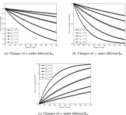
By utilising the proposed self-adaptive strategy, the three control parameters of particles in SAPSO can be adjusted in a way complying with the basic philosophies of the PSO development. Consequently, the proposed SAPSO is expected to improve the ability in finding high-quality solutions. Fig. 1 demonstrates the tendency of these changes in

125

the three control parameters with respect to different values ofβm. Note thatwmax=0.9,wmin=0.1,c1s=c2f=2.5,

c1f=c2s=0.5 andkmax=100 in this demonstration.

(5)

(a) Changes ofwunder differentβm (b) Changes ofc1under differentβm

(c) Changes ofc2under differentβm

Fig. 1. Changes of the three control parameters under differentβmin SAPSO

2.4. Analysis of trajectory in SAPSO

This subsection first analytically investigates the convergence of SAPSO. Then, a parameter selection principle guaranteeing the convergence of SAPSO is proposed.

130

2.4.1. Convergence analysis of SAPSO

Since each dimension of velocity and position vectors of each particle is updated independently from the others in Eq. (1) and Eq. (2), SAPSO can be simplified into a one-dimensional case for the analysis of its convergence property. For simplicity, we omit the subscriptmin Eq. (1) and Eq. (2). Then, the moving rules of particles in the one-dimensional SAPSO can be rewritten into a matrix form:

135 X(k+1) V(k+1) =A X(k) V(k) +BP (10) where A= 1−φ w −φ w (11) B= [φ φ]T (12) φ=φ1+φ2 (13) φ1=c1r1 (14) 140 φ2=c2r2 (15) P=φ1·pbest+φ2·gbest φ1+φ2 (16)

(6)

Solving|λE−A|=0 , whereEis the identity matrix with the same size ofA, the characteristic equation to the system Eq. (10) is derived as:

λ2−(w+1−φ)λ+w=0 (17)

where two roots, denoted byλ1,2, are obtained as:

λ1,2=

1+w−φ±p(1+w−φ)2−4w

2 (18)

In the context of the dynamic system theory, the necessary and sufficient condition for the convergence of the

145

system represented by Eq. (10) is that magnitudes ofλ1,2are less than 1 [33]. Thus, the system given by Eq. (10) converges if and only if:

Max{|λ1|,|λ2|}<1 (19)

From Eq. (18), it is clear thatλ1,2are either two real numbers or complex conjugates. Therefore, we investigate the convergence property in the two cases.

Case 1.λ1,2are complex numbers, i.e.λ1,2∈C.

150

Lemma 1. In the system represented by Eq. (10),λ1,2∈Cif and only if:

w−2√w+1<φ<w+2

√

w+1

w≥0 (20)

Proof. From Eq. (10), it is clear that:

λ1,2∈C⇔(1+w−φ)2−4w<0 (21)

Solving (21) by the classical mathematical approach, Lemma 1 can be easily proved.

Now, let us find conditions onφandwguaranteeing the convergence of the system given by Eq. (10) forλ1,2∈C. It is trivial that the system Eq. (10) converges if and only if Max{|λ1|,|λ2|}<1.

155

Lemma 2. Forλ1,2∈C, the system given by Eq. (10) converges, if and only if:

w−2√w+1<φ<w+2

√

w+1

0≤w<1 (22)

Proof. Note that the absolute value of a complex numberZcan be computed as|Z|= pZ2

r+Zc2, whereZr andZc denote the real and imaginary parts ofZ. Hence, forλ1,2∈C, we have:

Max{|λ1|,|λ2|}=|λ1|=|λ2|=√w (23)

Therefore:

Max{|λ1|,|λ2|}<1⇔

√

w<1 (24)

Forλ1,2∈C, Eq. (20) must hold according toLemma 1. From the two conditions, i.e. Eq. (20) and Eq. (24) , the

160

system represented by Eq. (10) converges, if and only if:

w−2√w+1<φ<w+2√w+1

0≤w<1 (25)

Case 2.λ1,2are two real numbers, i.e.λ1,2∈R.

(7)

Lemma 3. For the system given by Eq. (10),λ1,2∈Rif and only if:

φ∈R for w<0

φ≤w−2√w+1 orφ≥w+2√w+1 forw≥0 (26)

Proof. For the system in Eq. (10), it is clear that:

165

λ1,2∈R⇔(1+w−φ)2−4w≥0 (27)

Solving the right-hand side of Eq. (27) using the classical approach completes the proof.

Let us now investigateφ andwconditions for the convergence guarantee in Case 2. From Eq. (18) and Eq. (19), it is trivial, forλ1,2∈R, that the condition Max{|λ1|,|λ2|}<1 holds if and only if:

−1<1+w−φ± p (1+w−φ)2−4w 2 <1 (28) Hence: −3−w+φ<± q (1+w−φ)2−4w<1−w+φ (29)

Forλ1,2∈R, it is obvious that:

170 (28)⇔ −3−w+φ<−p(1+w−φ)2−4w p (1+w−φ)2−4w<1−w+φ (30)

Solving the right-hand side inequalities in Eq. (30), we have: (28)⇔

2w+2−φ>0

φ>0 (31)

Therefore, it is clear that, forλ1,2∈R, the system in Eq. (10) converges if and only if:

0<φ<2w+2, −1<w<0 0<φ≤w−2

√

w+1 orw+2√w+1≤φ<2w+2,0≤w<1 (32) Considering Case 1 and Case 2 together, the system represented by Eq. (10) converges if and only if:

0<φ<2w+2

−1<w<1 (33)

whereφ=φ1+φ2=c1r1+c2r2.

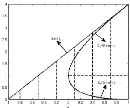
It is important to notice that the condition given by Eq. (33) is the necessary and sufficient condition for the

175

convergence of SAPSO. The convergence region denoted by Eq. (33) is shown in Fig. 2. For the parameter selection that locates wandφ in the convergence region given in Eq. (3), the trajectory convergence can be guaranteed in SAPSO.

(8)

Fig. 2. The convergence region for SAPSO

2.4.2. The equilibrium point of SAPSO

In the previous subsection, the convergence property of SAPSO is analytically investigated. Now, the remaining

180

task is to find the equilibrium point of SAPSO. Note that the equilibrium point is a stable point, to which particles converge. Calculating limits on both sides of Eq. (10) gives:

( _lim k→∞ X(k+1) =wlim k→∞ V(k) +φlim k→∞ (P−X(k)) lim k→∞ V(k+1) =lim k→∞ X(k) +lim k→∞ V(k) (34)

When SAPSO converges, it is clear that lim k→∞ X(k+1) =lim k→∞ X(k)and lim k→∞ V(k+1) =lim k→∞ V(k). Thus, substituting these two equations into Eq. (34), yields:

   lim k→∞ X(k) =P=φ1·pbest+φ2·gbest φ1+φ2 lim k→∞ V(k) =0 (35) whereφ1=c1r1andφ2=c2r2. 185

2.4.3. Convergence behaviour of particles in SAPSO

Before particles converge to the equilibrium point given in Eq. (35), they may exhibit different convergence behaviours depending on values ofwandφ. Four typical convergence behaviours of particles in SAPSO are shown in Fig. 3.

A non-oscillatory behaviour as shown in Fig. 3(a) leads particles to search only on one side of the equilibrium

190

point. Particles exhibit the non-oscillatory convergence behaviour whenλ1andλ2are two real roots and at least one of them is positive, which is equivalent to 0≤(1+w−φ)2−4wand 0<1+w−φ. The harmonic oscillation behaviour demonstrated in Fig. 3(b) occurs in the case whereλ1 andλ2are two complex roots, i.e. (1+w−φ)2−4w<0. Particles present zigzagging convergence behaviour shown in Fig. 3(c) when at least one ofλ1andλ2, has a negative real part, which is equal tow<0 or 1+w−φ<0. The combined harmonic with zigzagging behaviour illustrated in

195

Fig. 3(d) combines the harmonic and the zigzagging behaviours, which thus emerges when at least two complexλ1 andλ2roots has a negative real part, that is(1+w−φ)2−4w<0∩w<0∪(1+w−φ)2−4w<0∩1+w−φ<0. If boundaries of coefficients associated with these convergence behaviours are known beforehand, one may easily design an adaptive method to change values of these coefficients, so that the convergence of PSO can be guaranteed and the quality of the final solution can be improved.

200

(9)

(a) Non-oscillatory convergence (b) Harmonic convergence

(c) Zigzagging convergence (d) Harmonic combined with zigzagging Fig. 3. Convergence behaviour of particles in SAPSO

2.4.4. Convergence property of SAPSO with its stochastic nature

Due to its stochastic nature, it is difficult to rigorously establish an exact relationship between the stochastic nature and the convergence of SAPSO. However, one can still analyse the convergence property of SAPSO considering the bound of stochastic numbers used in SAPSO. Note that the stochastic nature of SAPSO is attributed to the existence of two random numbersr1andr2.

205

Sinceφ=φ1+φ2=c1r1+c2r2, the necessary and sufficient condition given by Eq. (33) can be rewritten as:

0<c1r1+c2r2<2w+2

−1<w<1 (36)

Lemma 4. SAPSO converges if:

   2w+2>c1+c2 −1<w<1 c1,c2>0 (37)

Proof. Becausec1andc2are two positive parameters, andr1andr2are two random numbers uniformly distributed

in[0,1], it is trivial thatc1≥c1r1andc2≥c2r2. Therefore:

   2w+2>c1+c2 −1<w<1 c1,c2>0 ⇒ 0<r1c1+r2c2<2w+2 −1<w<1 (38)

Since the right-hand side inequality in Eq. (38) is the necessary and sufficient condition for the convergence of

(10)

SAPSO, it is trivial that Lemma 4 holds.

2.4.5. Parameter selection principle in SAPSO

The following lemma provides a parameter selection principle, i.e. how to set the initial and final values ofw,c1 andc2, to guarantee the convergence in SAPSO.

Lemma 5. SAPSO converges if the initial and final values of the three control parameters of each particle satisfy the 215 following:    2wmin+2>c1s+c1f 1>wmax>wmin>−1 c1s=c2f>c1f =c2s>0 (39)

Proof. Whenc1s=c2f andc1f =c2s, it is clear from Eqs. (4)-(7) thatc1+c2=c1s+c1f for any particle at any

iteration in SAPSO. From Eqs. (3)-(5), it is trivial thatwmin≤w≤wmax,c1f ≤c1≤c1s andc2s≤c2≤c2f for any particle at any iteration in SAPSO. Therefore:

   2wmin+2>c1s+c1f 1>wmax>wmin>−1 c1s=c2f>c1f =c2s>0 ⇒    2w+2>c1+c2 −1<w<1 c1,c2>0 (40)

The right-hand side inequality in Eq. (40) is the sufficient condition for the convergence in SAPSO.

220

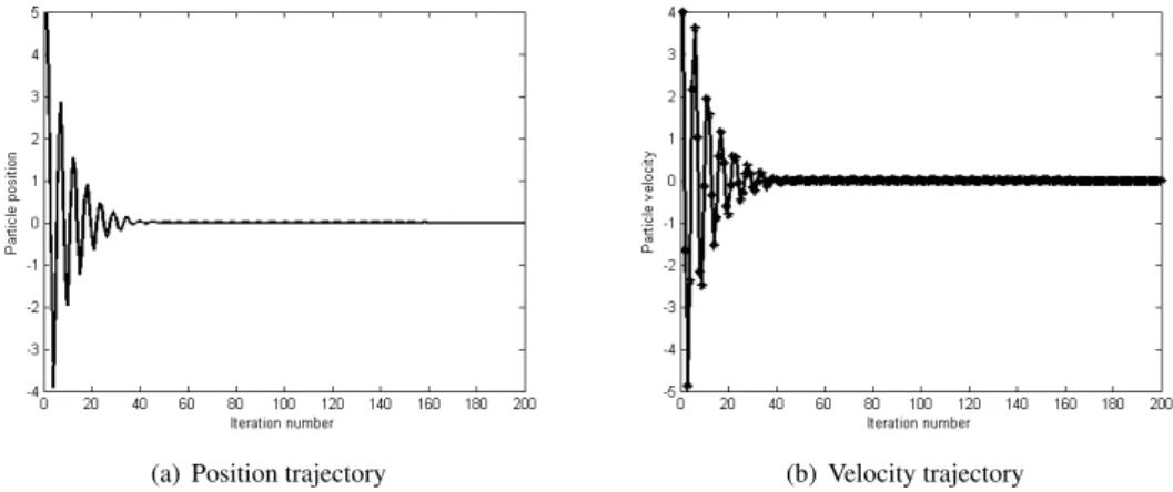
Lemma 5 implies that the convergence condition in SAPSO can be readily satisfied by setting the initial and final values of the three control parameters. Fig. 4 shows the convergence trajectories of the position and velocity of the particle under the suggested parameter selection:wmax=0.9,wmin=0.1,c1s=c2f=2 andc1f=c2s=0.1.

(a) Position trajectory (b) Velocity trajectory

Fig. 4. Convergence position and velocity trajectories of the particle in SAPSO under the suggested parameter selection

3. SAPSO-based MOO framework

3.1. The generality and some basic concepts of MOO 225

Generally, a MOO problem is to optimise a set of objectives subjecting to some equality/inequality constraints, which can be mathematically described as follows:

Optimize :F(x) = [f1(x),f2(x), ...,fQ(x)] (41) Subject to :      hi(x) =0 i=1,2, ...,CN1 (42) gj(x)<0 j=1,2, ...,CN2 (43) xl_k≤xk≤xku k=1,2, ...,n (44) 10

(11)

where fd (1≤d∈N≤Q) denotes thedth objective. Qis the total number of objectives andx= [x1,x2, ...,xn]is decision variable vector.nis the total number of decision variables.hi(x)denotes theith equality constraint andCN1 is the number of equality constraints. gj(x)represents the jth inequality constraint andCN2denotes the number of

230

inequality constraints.xl

kandxukrepresent the lower and upper bounds of thekth decision variable, respectively. For the completeness, some basic concepts of MOO stated in [6] are reproduced , especially for the minimisation problem.

Pareto dominance:SolutionS1is said to dominate solutionS2, denoted asS1S2, if and only if fd(S1)≤fd1(S2)

for alld∈[1,2, ...,Q]and∃d∈[1,2, ...,Q]such that fd(S1)<fd(S2).

235

Non-dominated solution:SolutionSis called a non-dominated solution (also called Pareto-optimal solution) if there exists no solution that can dominate solutionS.

Pareto set:The set of all non-dominated solutions is called the Pareto set.

Pareto front:The image of the Pareto set in the objective space is called the Pareto front.

3.2. Implementation of SAPSO for MOO 240

When using PSO to solve MOO problems, there are some key issues need to be addressed; (1) how to handle constraints of the MOO problem; (2) how to update the global and personal best solutions of particles; (3) how to keep the non-dominated solutions found by particles; (4) how to update the obtained non-dominated solution set. This subsection first addresses these mentioned key issues. Then, the proposed SAPSO-based MOO framework i.e., SAMOPSO, is described at the end of this subsection.

245

3.2.1. Handling constraints of MOO

Thanks to its simplicity and popularity, the constraint handling approach proposed in [34] is applied to handle constraints of the MOO problems. In this approach, the constraint violation degree of themth solution is calculated as [34]: violm= CN1

∑

i=1 |hi(x)|+ CN2

∑

j=1 max(0,gj(x)) (45)

whereCN1,hi(x),CN2andgj(x)have same definitions as those in Eqs. (42)-(43). |hi(x)|denotes the magnitude of

250 hi(x).

After calculating the constraint violation degree and fitness values of each solution, the constrained dominance rule described in [22] is implemented to select the non-dominated solution between any two candidate solutions in SAMOPSO. The constrained dominance rule can be summarised as follows: (1) for any two solutions with different constraint violation degrees, the solution with smaller constraint violation degree dominates the solution with larger

255

constraint violation degree; (2) for any two solutions with the same constraint violation degree, the precise Pareto dominance relationship described in the definition of “Pareto dominance” in Subsection 3.1 is used to select the non-dominated solution between those two candidate solutions.

It is clear that the constrained dominance rule considers infeasible solutions since they may still contain some valuable information of the solution space [22]. This could diversify the search for the non-dominated solutions and

260

reduce the possibility of missing important part of the solution space in the search. Consequently, it could increase the chance of finding the high-quality non-dominated solutions[22]. Note that, unless otherwise specified, the constrained dominance rule is applied to determine and select the non-dominated solution between any two candidate solutions in the developed SAMOPSO framework.

In the SAMOPSO framework proposed, the boundary constraints of each decision variable, given by Eq. (44),

265

is handled using a saturation strategy: the decision variablex_kfor allk∈ {1,· · ·,n}applies the following saturation strategy [18]: xk=    xl_k if xk<xlk xu_k if xk>xuk xk otherwise (46)

(12)

3.3. Updating the personal and global best solutions of particles

The personal and global best solutions in PSO-based MOO approaches are non-trivial from a set of non-dominated solutions generated. In this subsection, we address how to update the personal and global best solutions in our MOO

270

framework.

The personal best solution of a particle is referred to the best position that the particle searched so far and can be viewed as the memory of the particle. The proposed MOO framework utilises the conventional method applied in some other MOO research literature such as [5, 18, 21, 22] to update the personal best solution of each particle. In the conventional method, the personal best solution and the current solution of the particle are compared with each other

275

at each iteration. If the personal best solution of a particle dominates the current solution of the particle, the personal best solution is then kept; otherwise, the current solution becomes the personal best solution [5, 18, 21, 22].

Most of PSO-based MOO methods designs an external repository or archive to save the non-dominated solutions found [5, 18, 21, 22]. In the framework proposed in this paper, we also design a fixed-size external repository to save the non-dominated solutions. In addition, to efficiently determine the search directions of particles, the global best

280

solution of each particle is selected from the external repository using the geographically-based method [5].

In the geographically-based method [5], the search objective explored so far is firstly mapped into different grids. Then, the currently-found non-dominated solutions are located into a coordinate system using these girds, where each solution’s coordinates are defined based on its values of objective functions. After selecting a grid based on a density estimation operator, a non-dominated solution located in this grid is randomly selected as the global best solution [5].

285

Note that, in the density estimation operator, the more non-dominated solutions a grid contains, the less likely the grid is selected. This implies that the areas containing less non-dominated solutions are more likely to be selected [5]. Hence, particles are encouraged to explore the less crowed solution space. Consequently, we can increase the possibility to search less explored solution spaces and the chance of finding high-quality non-dominated solutions [5]. For more details about the geographically-based method, the reader is referred to [5].

290

3.4. Designing and updating the external repository

Because multiple non-dominated solutions are produced at each iteration in the developed MOO framework, the size of the repository could quickly increase if an external repository is designed to keep all the non-dominated solutions found. This could significantly increase the computation load in updating the repository as the current solutions of particles should be compared to the all non-dominated solutions saved in the repository. To mitigate this

295

issue, the size of the repository in the proposed SAMOPSO is fixed as in [5, 18, 21, 22]. For the repository with a fixed size, how to update the repository becomes important. Therefore, how our SAMOPSO updates the repository will be described in this subsection.

To update the external repository, we propose to combine the circular sorting approach with the elitist-preserving approach [4]. In the circular sorting method, the newly-found solution of a particle is first compared with its personal

300

best solution. If the new solution is non-dominated by the personal solution, it is allowed to be considered as a potential element of the repository.

Note that it is unnecessary to consider all new solutions as potential elements of the repository since they might be dominated by their personal best solutions. Therefore, sorting new solutions of individual particles by comparing them with their personal best solutions can relax the computational complexity in updating the repository.

305

The new solution sorted is then compared with all non-dominated solutions saved in the repository. The new solution is allowed to enter the repository if: (a) it is non-dominated by all non-dominated solutions in the repository or (b) it dominates any non-dominated solution saved in the repository (in this case, the dominated solutions are removed from the repository).

If the repository is full, the elitist-preserving approach [4] is applied. The elitist-preserving approach prunes the

310

repository to obtain a size-equaled repository and a well-distributed Pareto front. The approach first sorts all non-dominated solutions kept in the repository in an ascending order based on their function values. Then, the crowding distance of each non-dominated solution is calculated according to the objective functions of each non-dominated solution and those of its neighbors. Finally,Nrep non-dominated solutions with largest crowding distance are kept in the repository. Note that Nrep denotes the predefined size of the repository. The larger crowding distance the

315

non-dominated solutions have, the wider they are spread. Therefore, keeping the most sparely-spread non-dominated solutions in the repository can provide not only a size-equaled repository, but also a widely-distributed Pareto front [4, 6]. For more details of the elitist-preserving approach, the reader is referred to [4].

(13)

3.5. Algorithmic scheme of SAMOPSO

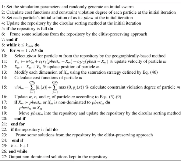
The algorithmic scheme of SAMOPSO is summarised in Table 1. In the scheme,NP,kandkmaxrepresent the size

320

of the swarm, the current iteration number and the maximum iteration number of the evolution, respectively. Table 1. The SAPSO-based MOO (SAMOPSO) framework

1: Set the simulation parameters and randomly generate an initial swarm

2: Calculate cost functions and constraint violation degree of each particle at the initial iteration 3: Set each particle’s initial solution of as itspbestat the initial iteration

4: Update the repository by the circular sorting method at the initial iteration 5:ifthe repository is fulldo

6: Prune some solutions from the repository by the elitist-preserving approach 7:end if

8:whilek≤kmaxdo 9: form=1 :NPdo

10: Selectgbestfor particlemfrom the repository by the geographically-based method

11: Vm←wVm+c1r1(pbestm−Xm) +c2r2(gbest−Xm)% update velocity of particlem

12: Xm←Xm+Vm% update position of particlem

13: Modify each dimension ofXmusing the saturation strategy defined by Eq. (46) 14: Calculate cost functions of particlem

15: violm= CN1

∑

i=1 |hi(x)|+ CN2

∑

j=1

max(0,gj(x))% calculate constraint violation degree of particlem 16: Updatew,c1andc2of particlemaccording to Eqs. (3)-(9)

17: ifXmpbestmorXmis non-dominated topbestmdo

18: pbestm=Xm

19: Move pbestminto the repository and update the repository by the circular sorting method

20: end if 21: end for

22: ifthe repository is fulldo

23: Prune some solutions from the repository by the elitist-preserving approach 24: end if

25: k←k+1 26:end while

27: Output non-dominated solutions kept in the repository

4. Numerical Experiments

4.1. Description of evaluation metrics

To allow a quantitative assessment of the performance of different MOO methods, this paper adopts five widely-accepted evaluation metrics: the number of non-dominated solutions (NNS) [5, 6, 18], error ratio (ER) [5, 6, 18],

325

generation distance (GD) [5, 6, 18], space metric (SM) [5, 6, 18] and the computation time (CT) [5, 6, 18]. The first four indices are mainly used to evaluate the quality of the obtained Pareto front [5, 6, 18]. NNSdenotes the number of real non-dominated solutions. The quality of the Pareto front obtained is better with a largerNNS[5, 6, 18]. ER

measures the non-convergence of the Pareto front toward the real Pareto front. The smaller theERvalue is, the better the convergence becomes. GDis a distance measure of the obtained non-dominated solutions from those in the real

330

Pareto front. The quality of the obtained Pareto front improves as theGDvalues decreases.SMis used to measure the uniformity in the spread of the Pareto front. The smaller theSMvalue becomes, the better the Pareto front solutions spread.CTis the computer execution time, which, to some extents, reflects the computational complexity of the MOO algorithm tested. Note that how to calculate these metrics is detailed in [5, 6, 18] .

(14)

4.2. Simulations on benchmark test functions 335

4.2.1. Description of benchmarks and compared MOO methods

In order to verify the proposed approach, its performance is evaluated using 12 well-known benchmark test func-tions extracted from [35, 6, 11, 12, 36] and one real-world engineering problem: environmental/economic dispatch (EED) problem. All benchmark test functions are described in Table 2. The performance of the proposed SAMOPSO is compared with those of NSGA-II [4], TV-MOPSO [18], BMOPSO [30] and MOEA/D [31]. For rigorous validation,

340

a Monte-Caro experiment with 30 runs is conducted for each test function. In addition, the non-dominated solutions of each method are obtained after 400 iterations of 100 particles in each studied case. All considered MOO methods are programmed by MATLAB 2012B software on a windows-8 personal computer with [email protected] and 2-GB RAM. For all MOO algorithms tested, the size of the external repository is set to be 100. The simulation parameters for SAMOPSO are given as:wmax=0.9,wmin=0.1,c1s=c2f =2.0 andc1f =c2s=0.1. These values are set based

345

on the convergence analysis results discussed in Section 2.4.5. The simulation parameters for all compared methods are extracted from their corresponding literature and summarised in Table 3.

Table 2. Benchmark test functions

Fun. Variable dimension Variable bounds Objective Function

F1 2 [0.1,1]∪[0,5] Function CONSTR in Ref. [4]

F2 2 [0,π]n Function TNK in Ref. [4]

F3 2 [0.1,1]n Test Function 4 in Ref. [5]

U F1 30 [0,1]×[−1,1]n−1 Refer to Ref. [36] U F2 30 [0,1]×[−1,1]n−1 Refer to Ref. [36] U F3 30 [0,1]n Refer to Ref. [36] ZDT1 30 [0,1]n Refer to Ref. [6] ZDT3 30 [0,1]n Refer to Ref. [6] DT LZ1 10 [0,1]n Refer to Ref. [35] DT LZ2 10 [0,1]n Refer to Ref. [35] DT LZ4 10 [0,1]n Refer to Ref. [35] DT LZ5 10 [0,1]n Refer to Ref. [35]

Table 3. The simulation parameters for compared methods

Methods Parameter setting

NSGA-II Pc=0.9,Pm=0.1

BMOPSO JP=0.001,α=6

MOEA/D F=0.5,Pc=0.5

TV-MOPSO wmax=0.7,wmin=0.4,c1s=c2f =2.5,c1f =c2s=0.5

4.2.2. Simulation results on 12 benchmark test functions

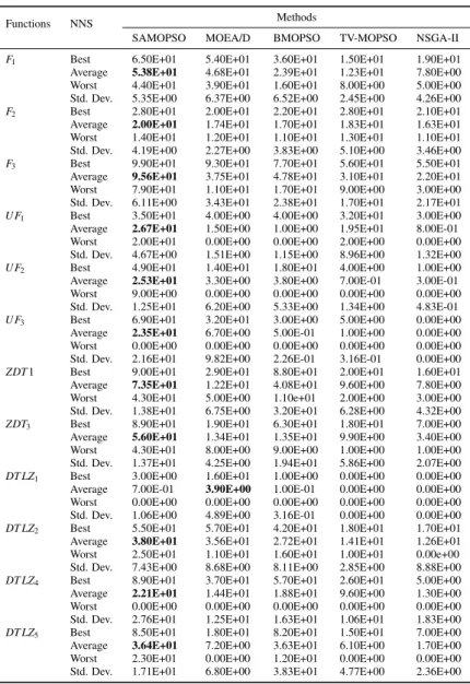
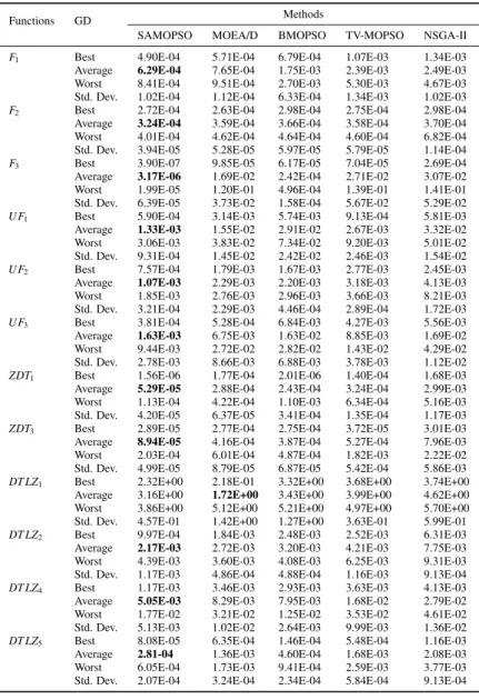
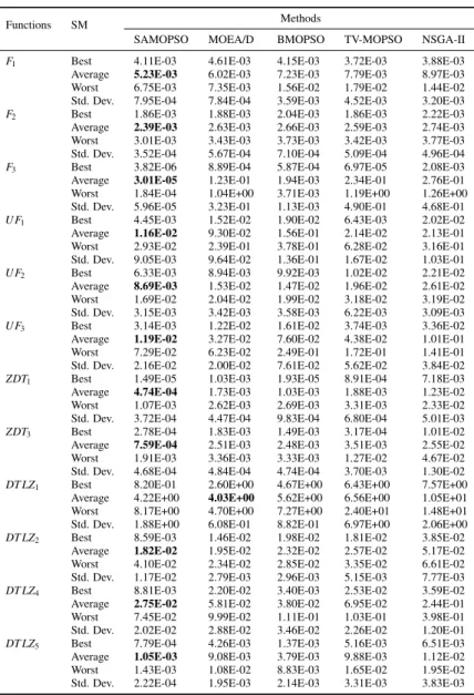
The statistical results of the Monte-Carlo experiments with respect to the five performance metrics are reported in Tables 4-8. In these tables, the best average results obtained with regarding to each metric are highlighted inboldface.

350

Note that the Pareto fronts obtained by different MOO algorithms are depicted inAppendix.

(15)

Table 4. Statistical results ofNNSobtained by different methods for different test functions

Functions NNS Methods

SAMOPSO MOEA/D BMOPSO TV-MOPSO NSGA-II

F1 Best 6.50E+01 5.40E+01 3.60E+01 1.50E+01 1.90E+01

Average 5.38E+01 4.68E+01 2.39E+01 1.23E+01 7.80E+00 Worst 4.40E+01 3.90E+01 1.60E+01 8.00E+00 5.00E+00 Std. Dev. 5.35E+00 6.37E+00 6.52E+00 2.45E+00 4.26E+00

F2 Best 2.80E+01 2.00E+01 2.20E+01 2.80E+01 2.10E+01

F3 Best 9.90E+01 9.30E+01 7.70E+01 5.60E+01 5.50E+01

U F1 Best 3.50E+01 4.00E+00 4.00E+00 3.20E+01 3.00E+00

Average 2.67E+01 1.50E+00 1.00E+00 1.95E+01 8.00E-01 Worst 2.00E+01 0.00E+00 0.00E+00 2.00E+00 0.00E+00 Std. Dev. 4.67E+00 1.51E+00 1.15E+00 8.96E+00 1.32E+00

U F2 Best 4.90E+01 1.40E+01 1.80E+01 4.00E+00 1.00E+00

Average 2.53E+01 3.30E+00 3.80E+00 7.00E-01 3.00E-01 Worst 9.00E+00 0.00E+00 0.00E+00 0.00E+00 0.00E+00 Std. Dev. 1.25E+01 6.20E+00 5.33E+00 1.34E+00 4.83E-01

U F3 Best 6.90E+01 3.20E+01 3.00E+00 5.00E+00 0.00E+00

Average 2.35E+01 6.70E+00 5.00E-01 1.00E+00 0.00E+00 Worst 0.00E+00 0.00E+00 0.00E+00 0.00E+00 0.00E+00 Std. Dev. 2.16E+01 9.82E+00 2.26E-01 3.16E-01 0.00E+00

ZDT1 Best 9.00E+01 2.90E+01 8.80E+01 2.00E+01 1.60E+01 Average 7.35E+01 1.22E+01 4.08E+01 9.60E+00 7.80E+00 Worst 4.30E+01 5.00E+00 1.10e+01 2.00E+00 3.00E+00 Std. Dev. 1.38E+01 6.75E+00 3.20E+01 6.28E+00 4.32E+00

ZDT3 Best 8.90E+01 1.90E+01 6.30E+01 1.80E+01 7.00E+00

DT LZ1 Best 3.00E+00 1.60E+01 1.00E+00 0.00E+00 0.00E+00

Average 7.00E-01 3.90E+00 1.00E-01 0.00E+00 0.00E+00 Worst 0.00E+00 0.00E+00 0.00E+00 0.00E+00 0.00E+00 Std. Dev. 1.06E+00 4.89E+00 3.16E-01 0.00E+00 0.00E+00

DT LZ2 Best 5.50E+01 5.70E+01 4.20E+01 1.80E+01 1.70E+01

Average 3.80E+01 3.56E+01 2.72E+01 1.41E+01 1.26E+01 Worst 2.50E+01 1.10E+01 1.60E+01 1.00E+01 0.00e+00 Std. Dev. 7.43E+00 8.68E+00 8.11E+00 2.85E+00 8.88E+00

DT LZ4 Best 8.90E+01 3.70E+01 5.70E+01 2.60E+01 5.00E+00

DT LZ5 Best 8.50E+01 1.80E+01 8.20E+01 1.50E+01 7.00E+00

(16)

Table 5. Statistical results ofERobtained by different methods for different test functions

Functions ER Methods

F1 Best 3.50E-01 4.60E-01 6.40E-01 8.50E-01 8.10E-01

Average 4.62E-01 5.32E-01 7.61E-01 8.77E-01 9.22E-01 Worst 5.60E-01 6.10E-01 8.40E-01 9.20E-01 9.50E-01 Std. Dev. 5.35E-02 6.37E-02 6.53E-02 2.46E-02 4.26E-02

F2 Best 7.20E-01 8.00E-01 7.80E-01 7.20E-01 7.90E-01

F3 Best 1.00E-02 7.00E-02 2.30E-01 4.40E-01 4.50E-01

U F1 Best 6.50E-01 9.60E-01 9.60E-01 6.80E-01 9.70E-01

Average 7.33E-01 9.85E-01 9.90E-01 8.05E-01 9.92E-01 Worst 8.0E-01 1.00E+00 1.00E+00 9.80E-01 1.00E+00 Std. Dev. 4.67E-02 1.51E-02 1.15E-02 8.96E-02 1.32E-02

U F2 Best 5.10E-01 8.60E-01 8.20E-01 9.60E-01 9.90E-01

Average 7.47E-01 9.67E-01 9.62E-01 9.93E-01 9.97E-01 Worst 9.10E-01 1.00E+00 1.00E+00 1.00E+00 1.00E+00 Std. Dev. 1.25E-01 6.20E-02 5.32E-02 1.34E-02 4.83E-03

U F3 Best 3.10E-01 6.80E-01 9.70E-02 9.50E-01 1.00E+00

Average 7.65E-01 9.33E-01 9.95E-02 9.90E-01 1.00E+00 Worst 1.00E+00 1.00E+00 1.00E+00 1.00E+00 1.00E+00 Std. Dev. 2.16E-01 9.82E-02 2.26E-03 3.16E-03 0.00E+00

ZDT1 Best 1.00E-01 7.10E-01 1.20E-01 8.00E-01 8.40E-01 Average 2.65E-01 8.78E-01 5.92E-01 9.04E-01 9.22E-01 Worst 5.70E-01 9.50E-01 8.90E-01 9.80E-01 9.70E-01 Std. Dev. 1.38E-01 6.75E-02 3.20E-01 6.28E-02 4.32E-02

ZDT3 Best 1.10E-01 8.10E-01 3.70E-01 8.20E-01 9.30E-01 Average 4.40E-01 8.66E-01 8.65E-01 9.01E-01 9.66E-01 Worst 5.70E-01 9.20E-01 9.10E-01 9.90E-01 9.90E-01 Std. Dev. 1.37E-01 4.25E-02 1.94E-01 5.86E-02 2.07E-02

DT LZ1 Best 9.70E-01 8.40E-01 9.90E-01 1.00E+00 1.00E+00

Average 9.93E-01 9.61E-01 9.99E-01 1.00E+00 1.00E+00 Worst 1.00E+00 1.00E+00 1.00E+00 1.00E+00 1.00E+00 Std. Dev. 1.06E-02 4.89E-02 3.16E-03 0.00E+00 0.00E+00

DT LZ2 Best 4.50E-01 4.30E-01 5.80E-01 8.20E-01 8.30E-01

Average 6.20E-01 6.44E-01 7.28E-01 8.59E-01 8.74E-01 Worst 7.50E-01 8.90E-01 8.40E-01 9.00E-01 1.00E+00 Std. Dev. 7.43E-02 8.68E-02 8.11E-02 2.85E-02 8.88E-02

DT LZ4 Best 1.10E-01 6.30E-01 4.30E-01 7.40E-01 9.50E-01

Average 7.79E-01 8.56E-01 8.12E-01 9.04E-01 9.87E-01 Worst 1.00E+00 1.00E+00 1.00E+00 1.00E+00 1.00E+00 Std. Dev. 2.76E-01 1.25E-01 1.63E-01 1.06E-01 1.83E-02

DT LZ5 Best 1.50E-01 8.20E-01 1.80E-01 8.50E-01 9.30E-01

Average 6.36E-01 9.28E-01 6.37E-01 9.39E-01 9.83E-01 Worst 7.70E-01 1.00E+00 8.80E-01 1.00E+00 1.00E+00 Std. Dev. 1.71E-01 6.80E-02 3.83E-01 4.77E-02 2.36E-02

(17)

Table 6. Statistical results ofGDobtained by different methods for different test functions

Functions GD Methods

F1 Best 4.90E-04 5.71E-04 6.79E-04 1.07E-03 1.34E-03

F2 Best 2.72E-04 2.63E-04 2.98E-04 2.75E-04 2.98E-04

F3 Best 3.90E-07 9.85E-05 6.17E-05 7.04E-05 2.69E-04

U F1 Best 5.90E-04 3.14E-03 5.74E-03 9.13E-04 5.81E-03

U F2 Best 7.57E-04 1.79E-03 1.67E-03 2.77E-03 2.45E-03

U F3 Best 3.81E-04 5.28E-04 6.84E-03 4.27E-03 5.56E-03

ZDT1 Best 1.56E-06 1.77E-04 2.01E-06 1.40E-04 1.68E-03

ZDT3 Best 2.89E-05 2.77E-04 2.75E-04 3.72E-05 3.01E-03

DT LZ1 Best 2.32E+00 2.18E-01 3.32E+00 3.68E+00 3.74E+00

Average 3.16E+00 1.72E+00 3.43E+00 3.99E+00 4.62E+00 Worst 3.86E+00 5.12E+00 5.21E+00 4.97E+00 5.70E+00 Std. Dev. 4.57E-01 1.42E+00 1.27E+00 3.63E-01 5.99E-01

DT LZ2 Best 9.97E-04 1.84E-03 2.48E-03 2.52E-03 6.31E-03

DT LZ4 Best 1.17E-03 3.46E-03 2.93E-03 3.63E-03 4.13E-03

DT LZ5 Best 8.08E-05 6.35E-04 1.46E-04 5.48E-04 1.16E-03

Average 2.81-04 1.36E-03 4.60E-04 1.68E-03 2.08E-03 Worst 6.05E-04 1.73E-03 9.41E-04 2.59E-03 3.77E-03 Std. Dev. 2.07E-04 3.24E-04 2.34E-04 5.84E-04 9.13E-04

(18)

Table 7. Statistical results ofSMobtained by different methods for different test functions

Functions SM Methods

F1 Best 4.11E-03 4.61E-03 4.15E-03 3.72E-03 3.88E-03

F2 Best 1.86E-03 1.88E-03 2.04E-03 1.86E-03 2.22E-03

F3 Best 3.82E-06 8.89E-04 5.87E-04 6.97E-05 2.08E-03

Average 3.01E-05 1.23E-01 1.94E-03 2.34E-01 2.76E-01 Worst 1.84E-04 1.04E+00 3.71E-03 1.19E+00 1.26E+00 Std. Dev. 5.96E-05 3.23E-01 1.13E-03 4.90E-01 4.68E-01

U F1 Best 4.45E-03 1.52E-02 1.90E-02 6.43E-03 2.02E-02

U F2 Best 6.33E-03 8.94E-03 9.92E-03 1.02E-02 2.21E-02

U F3 Best 3.14E-03 1.22E-02 1.61E-02 3.74E-03 3.36E-02

ZDT1 Best 1.49E-05 1.03E-03 1.93E-05 8.91E-04 7.18E-03

ZDT3 Best 2.78E-04 1.83E-03 1.49E-03 3.17E-04 1.01E-02

DT LZ1 Best 8.20E-01 2.60E+00 4.67E+00 6.43E+00 7.57E+00

Average 4.22E+00 4.03E+00 5.62E+00 6.56E+00 1.05E+01 Worst 8.17E+00 4.70E+00 7.27E+00 2.40E+01 1.48E+01 Std. Dev. 1.88E+00 6.08E-01 8.82E-01 6.97E+00 2.06E+00

DT LZ2 Best 8.59E-03 1.46E-02 1.98E-02 1.81E-02 3.85E-02

DT LZ4 Best 8.81E-03 2.20E-02 3.40E-03 2.53E-02 3.59E-02

DT LZ5 Best 7.79E-04 4.26E-03 1.37E-03 5.16E-03 6.51E-03

(19)

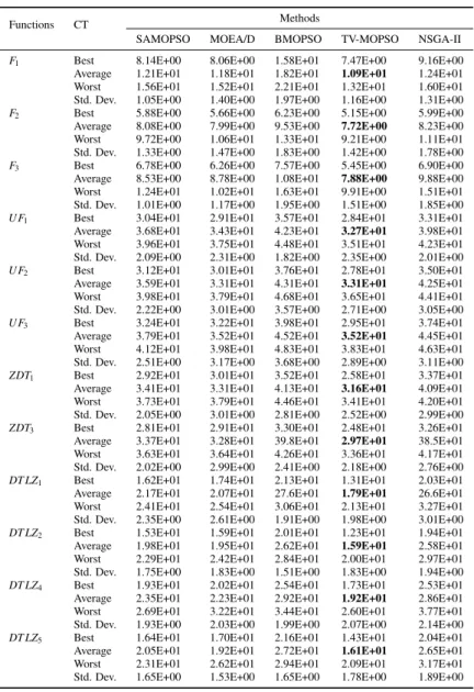
Table 8. Statistical results ofCT(seconds) obtained by different methods for different test functions

Functions CT Methods

F1 Best 8.14E+00 8.06E+00 1.58E+01 7.47E+00 9.16E+00

F2 Best 5.88E+00 5.66E+00 6.23E+00 5.15E+00 5.99E+00

F3 Best 6.78E+00 6.26E+00 7.57E+00 5.45E+00 6.90E+00

U F1 Best 3.04E+01 2.91E+01 3.57E+01 2.84E+01 3.31E+01

U F2 Best 3.12E+01 3.01E+01 3.76E+01 2.78E+01 3.50E+01

U F3 Best 3.24E+01 3.22E+01 3.98E+01 2.95E+01 3.74E+01

ZDT1 Best 2.92E+01 3.01E+01 3.52E+01 2.58E+01 3.37E+01

ZDT3 Best 2.81E+01 2.91E+01 3.30E+01 2.48E+01 3.26E+01

DT LZ1 Best 1.62E+01 1.74E+01 2.13E+01 1.31E+01 2.03E+01

DT LZ2 Best 1.53E+01 1.59E+01 2.01E+01 1.23E+01 1.94E+01

DT LZ4 Best 1.93E+01 2.02E+01 2.54E+01 1.73E+01 2.53E+01

DT LZ5 Best 1.64E+01 1.70E+01 2.16E+01 1.43E+01 2.04E+01

4.2.3. Analysis

From the statistical results ofNNS,ER,GDandSMreported in Tables 4-7, it can be observed that, our proposed method generally outperforms the four MOO algorithms compared over the majority of the benchmarks (except FunctionDT LT1). As shown in Tables 4-7, we can observe that all MOO methods cannot efficiently solve Function

355

DT LZ1. This could be interpreted by the complexities of objectives and many local optimal solutions contained in the

Pareto front of FunctionDT LZ1[35]. Nevertheless, MOEA/D and SAMOPSO outperforms the other three over this test function in terms of the average values of theNNS,ER,GDandSMmetrics.

From Table 8, it is evident that TV-MOPSO outperforms MOEA/D, SAMOPSO, NSGA-II and BMOPSO with respect to the average computation time. Since TV-MOPSO has the simplest updating rules in adjusting the three

360

control parameters of particles, its computation time is likely reduced. However, it is important to note that, despite consuming slightly more computation time than MOEA/D and TV-MOPSO, the proposed method provides the best performance in terms of the quality of Pareto front in most of the benchmark test functions as shown in Tables 4-7. Also, the difference in the average computation time between SAMOPSO, MOEA/D and TV-MOPSO is very small in all benchmark test functions. This implies that the computation time of SAMOPSO is comparable with those of

(20)

other MOO algorithms tested.

4.2.4. Statistical Comparison

This subsection performs a statistical comparison to detect whether the five tested methods are significantly dif-ferent in solving the 12 benchmarks. In the statistical comparison, a rank-based analysis is first conducted to examine the average rank of each method over the12 benchmark functions. Then, the non-parametric Friedman test [37] on

370

the mean rank followed by the pairwise post hoc Bonferroni-Dunn test [37] is performed to investigate the overall performances of different methods over the 12 test functions. Note that only theNNS metric is considered as an example in the statistical comparison. Following the same statistical comparison for the remaining three evaluation metrics, i.e.ER,GDandSM, we can readily analyse how much the five methods are significantly different from each other.

375

The ranks and average rank of each method for all benchmark functions are summarised in Table 9. From this table, SAMOPSO outperforms MOEA/D, BMOPSO, TV-MOPSO and NSGA-II with respect to the averageNNS

performance. Because this study compares 5 methods on 12 benchmark cases, the F-statistic value of the Friedman test at the confidence level of 90% equals to 2.0772. Note that the F-statistic value of the Friedman test at the confidence level of α% can be gained using the Matlab command: f inv(α,K−1,(K−1)(N−1)), whereK and

380

N, respectively, denote the number of methods and test functions. From Table 9, the obtained Friedman statistic value (Fscore) is equal to 31.6954. For more details about the calculation of Fscore, the reader is referred to [37]. Since theFscorevalue is bigger than the F-statistic value, the null hypothesis, i.e. each method equally performs over all considered benchmark problems, can be rejected [37]. This means that the five methods tested are significantly different over the 12 test functions at the confidence level of 90%.

385

Although the non-parametric Friedman test confirms that the five methods are significantly different over the 12 benchmark functions at the confidence level of 90%, it cannot be sufficiently concluded that SAMOPSO performs significantly better than the other four methods in terms of theNNSmetric. To highlight the mean performance of SAMOPSO with respect to the other four methods, the pairwise post hoc Bonferroni-Dunn test is performed in this paper. To examine whether or not a given method is significantly better than another method at the confidence level

390

ofα%, the Bonferroni-Dunn test checks whether the average rank difference between the two methods is greater than the critical difference value (CD). If it is true, we can conclude that the given method is significantly better than the other method at the confidence level ofα% [37]. Note that theCDvalue can be calculated byqα

p

K(K+1)/(6N)

forKmethods overNbenchmark test functions [37]. Here,qα is a constant parameter and is equal to 2.241 in this

study according to [37].

395

For the case where 5 methods are used to solve 12 test functions, we can readily obtain that, at the confidence level of 90%, the critical difference valueCDof the Bonferroni-Dunn test equals to 1.4466. From Table 9, it can be easily evaluated that the averageNNSvalue differences of SAMOPSO with respect to those of MOEA/D, BMOPSO, TV-MOPSO and NSGA-II are 1.5, 1.67, 2.5 and 3.83, which are all larger than the critical difference value of 1.4466. This implies that the proposed SAMOPSO provides significantly better averageNNSperformance than the four compared

400

methods over the 12 chosen benchmark problems at the confidence level of 90%. Following the same analysis, we can also conclude that SAMOPSO performs significantly better than its peers in terms of the meanER,GDandSM

performance over the 12 benchmarks at the confidence level of 90%.

(21)

Table 9. Rank values of averageNNSresults of different methods for 12 benchmarks (“AVR.” denotes the average rank value)

F1 1 2 3 4 5 F2 1 3 4 2 5 F3 1 3 2 4 5 U F1 1 3 4 2 5 U F2 1 3 2 4 5 U F3 1 2 4 3 5 ZDT1 1 3 2 4 5 ZDT3 1 3 2 4 5 DT LZ1 2 1 3 4 4 DT LZ2 1 2 3 4 5 DT LZ4 1 3 2 4 5 DT LZ5 1 3 2 4 5 AVR. 1.083 2.583 2.750 3.583 4.917

4.3. Application on the environmental/economic dispatch (EED) problem 4.3.1. Formulation of EED problem

405

Aiming to determine the optimal combination of power outputs of all generators over the whole scheduling period, the EED problem can be mathematically formulated as follows [17]:

minimise :

(

F=∑Ni=1(ai+biPi+ciPi2)

E=∑Ni=1(αi+βiPi+γiP_i2+ξiexp(λiPi))

(47) Subject to :                Pi,min≤Pi≤Pi,max (48) N

∑

i=1 Pi=PL+PD (49) PL= N

∑

i=1 N

∑

j=1 PiBi jPj+ N

∑

i=1 PiBi0+B00 (50)

whereF denotes the total fuel cost in $/h. E represents the total emission rate inKg/h. ai,bi andciare fuel cost coefficients of generatori.βi,γi,ξiandλiare emission coefficients of generatori.Piis the power output of generator

410

iinMW.Ndenotes the total number of generators.Pi,minandPi,maxdenote the minimum and maximum output limits of generatori, respectively. PLis the total power loss of the power system inMW. PDis the total power demand of the system inMW.Bi j,Bi0andB00represent the transmission loss coefficients.

4.3.2. Numerical simulation for the EED problem

SAMOPSO, MOEA/D, BMOPSO, TV-MOPSO and NSGA-II are applied to solve the IEEE-30-bus system [38]

415

with 6 generators. In the numerical simulation, a Monte-Carlo experiment with 30 runs is conducted. The size of the repository of each method is bounded to be 50 in each run of the Monte-Carlo experiment. The total power demand of the system is given asPD=2.2. The minimum and maximum output boundaries for the 6 generators are set to be

Pmin= [0.05,0.05,0.05,0.05,0.05,0.05]andPmax= [0.5,0.6,1.0,1.2,1.0,0.6], respectively. The other coefficients for the IEEE-30-bus system are given as follows:

420

B00=0.0014 (51)

(22)

Bi j=         0.0218 0.0107 −0.00036 −0.0011 0.00055 0.0033 0.0107 0.01704 −0.0001 −0.00179 0.00026 0.0028 −0.0004 −0.0002 0.02459 −0.01328 −0.0018 −0.0079 −0.0011 −0.00197 −0.01328 0.0265 0.0098 0.0045 0.00055 0.00026 −0.0118 0.0098 0.0216 −0.0001 0.0033 0.0028 −0.00792 0.0045 −0.00012 0.02978         (53)

Table 10. The fuel cost and emission coefficients of each generator of the IEEE-30-bus system (Gidenotes theith generator)

G1 G2 G3 G4 G5 G6 a 10 10 20 10 20 10 b 200 150 180 100 180 150 c 100 120 40 60 40 100 α 4.091 2.543 4.258 5.526 4.258 6.131 β -5.554 -6.047 -5.094 -3.55 -5.094 -5.555 γ 6.490 5.638 4.586 3.380 4.586 5.151

ξ 2e-04 5e-04 1e-06 2e-03 1e-06 1e-05

λ 2.857 3.333 8.000 2.000 8.000 6.667

The statistical results of the tested MOO algorithms, with respect to the five performance metrics, are summarised in Table 11. The non-dominated solutions produced by different methods are visualised in Fig. 5. From Table 11, it is clear that SAMOPSO outperforms other four algorithms in terms of the averageNNS,ER,GDand SM 425

performance in the EED problem. Comparing with MOEA/D, BMOPSO, TV-MOPSO and NSGA-II, SAMOPSO averagely improves the NNS performance by 97.87%, 153.64%, 298.57% and 654.05%; theER performance by 38.44%, 43.33%, 48.60% and 52.27%; theGDperformance by 50.71%, 53.99%, 55.41% and 55.57% and the SM

performance by 49.76%, 54.22%, 57.26% and 57.96%, respectively. This confirms that that SAMOPSO provides better quality of the Pareto front for the EED problem, compared with its competitors.

430

As shown in Table 11, TV-MOPSO, MOEA/D and SAMOPSO are ranked the first, second and third in terms of the computation time, but the difference is small. Here, it is important to note that, despite taking slightly more computation time than MOEA/D and TV-MOPSO, SAMOPSO significantly outperforms these two methods with respect to the meanNNS,ER,GDandSMperformance.

Table 11. Statistical results of different evaluation metrics obtained by different methods for the EED problem

Metrics Methods

NNS Best 4.90e+01 2.90E+01 2.70E+01 1.70E+01 8.00E+00 Average 2.79E+01 1.41E+01 1.10E+01 7.00E+00 3.70E+00 Worst 6.00E+00 4.00E+00 4.00E+00 2.00E+00 1.00E+00 Std. Dev. 1.83E+01 1.16E+01 8.69E+00 4.50E+00 2.00E+00

ER Best 2.00E-02 4.20E-01 4.60E-01 6.60E-01 8.40E-01 Average 4.42E-01 7.18E-01 7.80E-01 8.60E-01 9.26E-01 Worst 8.80E-01 9.20E-01 9.20E-01 9.60E-01 9.80E-01 Std. Dev. 3.66E-01 2.31E-01 1.74E-01 8.99E-02 4.01E-02

GD Best 7.40E-04 1.44E-02 1.88E-02 1.21E-02 1.45E-02 Average 1.73E-02 3.51E-02 3.76E-02 3.88E-02 3.91E-02 Worst 3.59E-02 7.53E-02 7.96E-02 1.44E-01 1.21E-01 Std. Dev. 1.31E-02 1.94E-02 2.16E-02 3.89E-02 3.33E-02

SM Best 5.24E-03 7.54E-02 9.69E-02 7.97E-02 7.37E-02 Average 1.03E-01 2.05E-01 2.24E-01 2.41E-01 2.45E-01 Worst 2.47E-01 4.99E-01 5.42E-01 8.15E-01 9.94E-01 Std. Dev. 8.05E-02 1.41E-01 1.61E-01 2.33E-01 2.76E-01

CT Best 3.33E+01 3.20E+01 3.76E+01 3.03E+01 3.87E+01 Average 3.72E+01 3.61E+01 3.82E+01 3.41E+01 4.15E+01 Worst 4.01E+01 3.92E+01 4.44E+01 3.69E+01 4.52E+01 Std. Dev. 1.15E+00 1.12E+00 1.35E+00 1.01E+00 1.59E+00

(23)

500 550 600 650 700 18.7 18.8 18.9 19 19.1 19.2 19.3 19.4 Fule Cost($/h) Emission(Kg/h) SAMOPSO MOEA/D BMOPSO TV−MOPSO NSGA−II Pareto Front 555 560 19.06 19.07 19.08

Fig. 5. Pareto fronts obtained by different methods for the EED problem

5. Conclusions

435

In this study, a PSO-based MOO framework is developed to obtain a high-quality Pareto front. For this pur-pose, a novel PSO method, named self-adaptive PSO (SAPSO), is first proposed and implemented to search the non-dominated solutions in the developed MOO framework. In order to well balance the trade-offs between the exploration and exploitation capabilities of SAPSO, we propose a self-adaptive strategy that tunes the three control parameters of particles. Since the convergence property of PSO plays a crucial role in the field of PSO development,

440

this paper also investigates the convergence of the proposed SAPSO method with respect to different values of the three control parameters. Then, a convergence-guaranteed parameter selection principle is proposed for the developed SAPSO.

Leveraging the proposed SAPSO, this paper completes the design of a MOO framework, called SAMOPSO. In the proposed framework, a fixed-size external repository is designed to save non-dominated best solutions of particles.

445

To obtain a well-distributed Pareto front, this paper develops the circular sorting method, which is integrated with the elitist-preserving approach [4] and updates the external repository.

The proposed approach is validated via 12 benchmark test functions and a real-world MOO problem against four well-established MOO algorithms: MOEA/D, BMOPSO, NSGA-II and TV-MOPSO. The comparison is conducted based on five widely-adopted MOO performance metrics. The simulation results reveal that the proposed method is

450

highly competitive in most of benchmark test functions with respect to the quality of the Pareto front. Moreover, the statistical analysis on the simulation results verifies that the proposed method significantly outperforms the other four compared algorithms in the selected benchmark problems at the confidence level of 90%. Also, the computation time of the proposed method is comparable with those of the other methods. This implies that the proposed framework is a very effective MOO algorithm.

455

Appendix

(24)

0.4 0.5 0.6 0.7 0.8 0.9 1 1 2 3 4 5 6 7 8 9 f1 f2 SAMOPSO MOEA/D BMOPSO TV−MOPSO NSGA−II Pareto Front 0.5 0.55 0.6 3.5 4 4.5 0.52 0.53 0.54 4.3 4.4 4.5 (a) FunctionF1 0 0.2 0.4 0.6 0.8 1 1.2 1.4 0 0.2 0.4 0.6 0.8 1 1.2 1.4 f1 f2 SAMOPSO MOEA/D BMOPSO TV−MOPSO NSGA−II Pareto Front 0.46 0.48 0.5 0.86 0.87 0.88 0.89 0.9 (b) FunctionF2 0.1 0.2 0.3 0.4 0.5 0.6 0.7 0.8 0.9 1 0 1 2 3 4 5 6 7 8 f1 f2 SAMOPSO MOEA/D BMOPSO TV−MOPSO NSGA−II Pareto Front 0.26 0.27 0.28 0.29 2.5 2.55 2.6 2.65 2.7 2.75 (c) FunctionF3 0 0.2 0.4 0.6 0.8 1 0 0.2 0.4 0.6 0.8 1 1.2 f1 f2 SAMOPSO MOEA/D BMOPSO TV−MOPSO NSGA−II Pareto Front 0.3 0.31 0.32 0.33 0.43 0.44 0.45 0.46 (d) FunctionU F1 0 0.2 0.4 0.6 0.8 1 0 0.2 0.4 0.6 0.8 1 1.2 f1 f2 SAMOPSO MOEA/D BMOPSO TV−MOPSO NSGA−II Pareto Front 0.26 0.28 0.48 0.5 (e) FunctionU F2 0 0.2 0.4 0.6 0.8 1 0 0.2 0.4 0.6 0.8 1 1.2 f1 f2 SAMOPSO MOEA/D BMOPSO TV−MOPSO NSGA−II Pareto Front (f) FunctionU F3

Fig. 6. Pareto fronts obtained by different methods for different Functions

(25)

0 0.2 0.4 0.6 0.8 1 0 0.2 0.4 0.6 0.8 1 1.2 f1 f2 SAMOPSO MOEA/D BMOPSO TV−MOPSO NSGA−II Pareto Front 0.27 0.28 0.29 0.3 0.46 0.47 0.48 0.49 (a) FunctionZDT1 0 0.1 0.2 0.3 0.4 0.5 0.6 0.7 0.8 0.9 −0.8 −0.6 −0.4 −0.2 0 0.2 0.4 0.6 0.8 1 f1 f2 SAMOPSO MOEA/D BMOPSO TV−MOPSO NSGA−II Pareto Front 0.2 0.21 0.22 0.46 0.48 0.5 (b) FunctionZDT3 0 10 20 30 0 10 20 30 0 5 10 15 20 25 30 f2 f1 f3 SAMOPSO MOEA/D BMOPSO TV−MOPSO NSGA−II Pareto Front (c) FunctionDT LZ1 (d) FunctionDT LZ2 (e) FunctionDT LZ4 0 0.2 0.4 0.6 0.8 0 0.2 0.4 0.6 0.8 0 0.5 1 1.5 f2 f1 f3 SAMOPSO MOEA/D BMOPSO TV−MOPSO NSGA−II Pareto Front 0.64 0.66 _{0.64 0.645}0.65 0.655 0 0.5 (f) FunctionDT LZ5

Fig. 7. Pareto fronts obtained by different methods for different Functions

References

[1] M. Arsuaga-R´ıos, M. A. Vega-Rodr´ıguez, F. Prieto-Castrillo, Meta-schedulers for grid computing based on multi-objective swarm algorithms, Applied Soft Computing Journal 13 (4) (2013) 1567–1582.