Rep. Prog. Phys.64(2001) 97–146 www.iop.org/Journals/rp PII: S0034-4885(01)04040-4
Solar neutrinos
Michael F Altmann1,3, Rudolf L M¨oßbauer2and Lothar J N Oberauer2
1Max-Planck-Institut f¨ur Physik (Werner-Heisenberg-Institut), 80805 M¨unchen, Germany 2Technische Universit¨at M¨unchen, Physik Department E15, 85747 Garching, Germany E-mail: [email protected]
Received 9 November 2000
Abstract
Within the last decade solar neutrino physics has evolved into a field of relevance not only for probing our understanding of stellar physics, but also for investigating and pinpointing intrinsic neutrino properties, most importantly neutrino masses and mixing angles. To date, results from six different and partly complementary experiments have been acquired. Taken together, these experimental data provide evidence for neutrino oscillations, i.e. neutrino masses and mixing, and thus physics beyond the standard model of electroweak interactions. Several new experiments currently being planned or constructed will commence operation within the next few years. They will provide additional complementary data and allow—together with the already running detectors—performance of a full solar neutrino spectroscopy in both the charged-current and the neutral-current detection mode. Performing a thorough comparison of the spectral shape observed on Earth and the neutrino spectrum expected from solar model computations will be essential for further pinpointing neutrino masses and mixing parameters. This article, after giving a short introduction to the field, reviews the current status of solar neutrino physics and gives an outlook on the potential which the upcoming experiments offer for further progress.
3 Author to whom any correspondence should be addressed.
Contents
Page
1. Solar neutrino physics: history 99
2. Neutrino oscillations 100
2.1. Neutrino masses and mixing 100
2.2. Neutrino oscillations in vacuum 101
2.3. Matter-enhanced oscillations 103
3. Solar neutrino production 106
3.1. Basic ideas of the solar model 106
3.2. Thermonuclear processes: pp and CNO cycles 107
3.3. Uncertainties and accuracy of neutrino flux predictions 112
4. Solar neutrino detection 114
4.1. Charged-current and neutral-current detection 114
4.2. General detector requirements 115
4.3. Solar neutrino experiments: an overview 116
4.4. Operating experiments and their results 117
5. Implications 127
5.1. The solar neutrino puzzle 127
5.2. Deficit of8B neutrinos 128
5.3. Deficit of7Be neutrinos—a hint of oscillations 129
5.4. Neutrino oscillation scenarios 129
5.5. A way to pinpoint neutrino parameters—solar neutrino spectroscopy 131
6. Prospects: future solar neutrino experiments 133
6.1. BOREXINO 133
6.2. KAMLAND 137
6.3. GNO upgrade: GNO-66 and GNO-100 138
6.4. The day–night effect in the Homestake iodine experiment 139
6.5. The far future 140
7. Conclusions 142
Acknowledgments 142
1. Solar neutrino physics: history
Neutrinos, being neutral particles, are subject only to the weak interaction (and gravity). Therefore their detection in terrestrial detectors of at most a few hundred tons of material becomes very difficult.
Neutrinos were first introduced into physics as hypothetical particles by Wolfgang Pauli in 1930; see [114]. Pauli had to cope at that time with the fact that electrons emitted in ordinary radioactive decays exhibited a continuous spectrum, suggesting the introduction of a three-body rather than a two-body decay. His theory had been formulated, however, before the discovery of the neutron. A two-particle decay led to a statistics which was not in agreement with the results of optical spectroscopy, while a three-particle decay could explain the continuous form of the electron spectrum and yielded the right statistics, but gave rise to a series of other problems, which were only solved in 1932 with the discovery of the neutron by Chadwick [36]. The third particle, which had been introduced by Pauli to add to the proton and electron, was finally called the neutrino by Fermi, meaning ‘little neutron’ in Italian. Though the existence of the neutrino had been seen earlier in recoil experiments [122], it remained for Fred Reineset al[41, 121], in about 1956, to discover the neutrino in an actual reaction. This reaction, which even nowadays is still used in antineutrino observations, reads in modern language p + ¯νe → n + e+. This first discovery of the neutrino won Reines the Nobel Prize in 1995.
While complete parity conservation would require neutrinos to be of both helicities, complete parity violation would involve only one helicity, as has been observed experimentally by Goldhaberet al[74], according to whom neutrinos are emitted with only left-handed helicity,
νL. This follows nowadays also from the standard theory SU(2)Lof electroweak interactions. This theory assumes that onlyνL andν¯R feel the weak forces. Thus, only the left-handed fermions form doublets:
(u,d)L (c,s)L (t,b)L
(νe,e−)L (νµ, µ−)L (ντ, τ−)L
where the use of primes indicates that we are referring to the weak eigenstates of the down, strange, and beauty quarks, which result from the mass eigenstates (d,s,b) via a unitary transformation. The right-handed fermions, which do not participate in the weak interactions, are singlets. We shall use the notation for chiralityνL=(1 +γ5)νandν¯R =(1 +γ5)ν¯, where
γ5=
3 i=0γi.
Lederman, Schwartz, and Steinberger discovered in 1962 the existence of a second type of neutrino [47]. Today we know that there are only three types of light neutrino. This knowledge arises from experiments at CERN [32, 33], which measured the total width of the Z0 resonance, attributing widths to six quarks, three charged leptons, and three light neutral leptons, assuming the latter to have equal width. This procedure does not exclude heavier neutrinos withmν 45 GeV. The three types of light neutrino are calledνe(electron neutrino),
νµ(muon neutrino), andντ(tau neutrino).
While we know a lot about the quarks and the charged leptons, we still know very little about the neutrinos, including their mass values. Direct measurements of neutrino masses due to their extremely small values yield at present only limits: m(νe) <2.2 eV (95% c.l.) [144],
m(νµ) <0.16 MeV (90% c.l.) [12],m(ντ) <18.2 MeV (95% c.l.) [33].
There also exists a theoretical mass limit for neutrinos of cosmological origin: attributing the entire mass of the Universe to neutrinos only, and adding for safety reasons a factor of two to the critical mass of the Universe, we arrive at a theoretical mass limit, which is given by
3
Information on the masses of neutrinos is available from three types of experiment: (a) Direct determination of masses from kinematical experiments (energy and momentum
balance).
(b) Neutrinoless doubleβ-decay (0ν–ββdecay). (c) Neutrino oscillations.
As will be elucidated in the following section, neutrino oscillations in particular, being a quantum mechanical interference effect, open the prospect of detecting even tiny mass differences between neutrino eigenstates. Using electron neutrinos emitted by the Sun, neutrino masses down tomν10−6eV can be investigated.
2. Neutrino oscillations
2.1. Neutrino masses and mixing
Neutrino oscillations are oscillating transitionsνα ↔νβ (α, β =e, µ, τ), where one kind of neutrino transfers into another kind of neutrino distinguished by different leptonic quantum numbers. We are usually dealing with ‘flavour’ oscillations, where the total lepton number is conserved, L = 0, and only conservation of the family lepton numbers Lα is violated. The idea of neutrino oscillations of the type particle ↔ antiparticle (ν ↔ ¯ν) was first introduced in 1958 by Pontecorvo [115], i.e. long before the observation of the second type of neutrino. The idea of the mixing of massive neutrinos was introduced in 1962 by Maki [110]. Two-flavour oscillations were also discussed by Pontecorvo in 1967 [116, 117]. A consistent phenomenological theory of neutrino mixing and oscillations was developed in 1969 by Gribov and Pontecorvo [79]. In the case of quarks, such mixing and the associated oscillations are well known. Here it is observed, though theoretically not understood, that the eigenstates(d,s,b)entering the weak charged current are orthonormal linear combinations of the energy eigenstates(d,s,b)of quarks. The weak eigenstates are thereby those states which are produced in weak decays, while the energy eigenstates are those states which determine the propagation of particles in the vacuum, i.e.
|ν(t, x) = |ν(0)exp(−i(Et− p·x)).
The relation between the two kinds of eigenstate is given by the Cabibbo–Kobayashi–Maskawa mixing matrix: d s b = U d1 Ud2 Ud3 Us1 Us2 Us3 Ub1 Ub2 Ub3 d s b .
This connection is linear as a consequence of basic principles of quantum mechanics. Due to redundancies, it is sufficient to write this relation between either the upper or lower states of the quark families, where for quarks the lower states have been chosen. The nine complex coefficients of the mixing matrix reduce to nine real coefficients because of the unitarity condition. Again because of redundancies, these are reduced further to four parameters, three being mixing angles and one being a phase. There appears no physical reason that such a connection should not exist also for leptons. Again because of redundancies, one might write such a relation for either the upper or lower states of the leptons, where it is customary to use the upper states, i.e. the neutrinos, in order to leave the mass determinations of the charged
leptons unchanged. Like in the case of quarks, there are only four relevant parameters in the mixing matrix.
Two conditions are necessary for the appearance of neutrino oscillations: (1) Lepton family quantum numbers are not strictly conserved,Lα=0.
(2) At least two neutrinos differ in their mass values. If all neutrino masses are equal (i.e. complete degeneracy, mi = m), then νβ|M|να = mδαβ because of unitarity. Oscillatory transitionsνα↔νβwould then be impossible.
Because neutrino oscillations exist only if neutrino masses exist, there is apparently a close connection between neutrino oscillations and neutrino masses. The question arises here of why neutrinos should have any mass value at all. Neutrinolessββ-processes, which would imply a lower bound on neutrino mass, have not yet been observed. This fact does not, however, imply an upper bound on the mass of the neutrinos, because the matrix elements may exhibit cancellations. Neutrinos appear in weak interactions only with definite chirality. Massive neutrinos, on the other hand, require both chiralities, which would require a deviation from the present standard model. Such a deviation, nevertheless, is possible. Massive neutrinos might also partially be candidates for the missing dark matter in the Universe. They furthermore might settle the question of whether the Universe is open, closed or flat. The rest mass of the photon is zero, which is a consequence of the gauge invariance of the electromagnetic interaction. For neutrinos, however, there is no similar invariance principle known. It furthermore has to be explained why neutrino masses (if they exist) are much smaller than the masses of charged leptons. The seesaw principle offers a remedy, yet at the expense of the introduction of Majorana neutrinos.
2.2. Neutrino oscillations in vacuum
There are two types of experiment which might be envisaged:
(1) Appearance experiments, where one searches for the appearance of states with a new flavour in a beam. Such experiments are by necessity particularly sensitive to mixing parameters.
(2) Disappearance experiments, where one looks for the disappearance of neutrinos of the initial flavour from a beam. Such experiments might involve, in particular, electron neutrinos, in case there is not sufficient energy available to create neutrinos of another kind. Such is the situation with reactor-produced neutrinos and solar neutrinos, whose energy is far below the rest masses of the chargedµ- andτ-leptons. These kinds of experiment are particularly sensitive to small energies and therefore also to small mass values. For solar neutrinos, only the experimental situation (2) is feasible for energetic reasons. In the scheme with neutrino mixing, the neutrino flavour states are coherent superpositions of the state vectors of neutrinos with different masses. This is the basic quantum mechanical reason for the phenomenon of oscillations. We shall therefore discuss the problem of coherence: non-degenerate mass eigenstates propagate with different velocities and must therefore have been emitted at different times or places if they arrive on Earth at the same time or in the same place. Interference between different mass eigenstates will only occur if the source remains coherent over a time interval comparable to the difference in arrival times. The quantum mechanical condition for such an interference is(v1−v2)t cτcoh. Here,t is the transit time of photons for the distanced between the Sun and the Earth,t ≈d/c, whilevi is the transit velocity of theith massive component between the Sun and the Earth andτcoh is the coherence time within the Sun, which is essentially given by the collision time for one proton with another. The times involved differ somewhat according to author: we have Nussinov
et al[113], who arrives for mere proton–proton collisions at valuesτcoh=10−17s, Kraus and Wilczek [99], who arrive atτcoh=10−15s, taking into account that we are really dealing with a plasma, where collisions between protons and electrons matter, and Loeb [108], who arrives at 5×10⁻¹⁵s, by writing down all effects and coming to the conclusion that proton–proton collisions dominate. In any case, we obtain in all theories for the vacuum oscillations in the Sun–Earth distance full coherence for the8B neutrinos and even more so for all neutrinos of lower energy. For the energies within the Sun where we might have the MSW effect to be described below; full coherence is even more definitely present. It should be noted that the problem of coherence was also treated by Stodolsky [132], who came to the conclusion that the energy spectrum already contains all pertinent information.
If neutrinos appear in a mixed state, then we may have neutrino decay. The absence of
γ-rays from SN1987A shows, however, that the lifetimes of solar neutrinos are sufficiently long to consider them to be constant. Neutrino oscillations like quark oscillations have the prerequisite that eigenstates of the energy (or mass, in the case where the momentum of a neutrino beam can be considered constant) and weak-interaction eigenstates differ, i.e. that their relation has non-diagonal matrix elements. We shall discuss such oscillations now in the presence of three neutrino statesνe,νµ,ντ. The connection is (for quantum mechanical
reasons) given by a unitary transformationU, which is also called the mixing matrix: |να =
i
Uαi|νi
and the inverse |νi = α (U†) iα|να = α U αi|να whereU†U =1.
We shall in the following assume neutrino masses to all have the same momentum state, i.e. we shall assume the neutrino beams to have a common momentum. Being eigenstates of the mass matrix, the states are stationary states, i.e. they have a time dependence4
νi(t)=exp(−iEit)νi(t=0) where Ei = p2 ν+m2i ≈pν+m2i/(2pν)≈Eν+m2i/(2Eν)
and we have assumed pν mi, i.e. highly relativistic neutrinos. A pure flavour beam
να(0)=ναat time zero thus would develop over time into the beam
ν(t)= i
Uαiexp(−iEit)νi =
i,β
UαiUβi exp(−iEit)νβ.
One usually measures probabilities. The probability of findingνβ atL ≈ t for light (i.e. relativistic) neutrinos is given by
P (να→νβ)=
i
UαiUiβ† exp
−im 2 i 2pνt 2 (1) = i |UαiUiβ2|2+ Re i j=i
UαiUiβ†UαjUjβ† exp
im 2 ijL 2Eν (2) wherem2 ij = |m2i −m2j|.
A straightforward calculation yields in the two-neutrino approximation for the probabilitiesP of observing a neutrino of typeνβ, if one has started at the origin with neutrino typeνα, P (να→νβ)=P (ν¯α→ ¯νβ)= 1 2sin 22θ 1−cosm 2t 2Eν (3) = sin22θsin2 1.27(m 2/eV2)(L/m) (Eν/MeV) (4)
if practical units are used andα=β.
This relation clearly shows the oscillatory behaviour of the neutrino oscillations, where one starts with one kind of neutrino and generates either new types of neutrino (α =β) or simple deviations of the neutrinos from ordinary expectations (α = β). It should be noted in this context that in the oscillatory probability, smaller values ofm2require larger values of the distanceL. The expression for neutrino oscillations yields the normalized transition probability for neutrino oscillations:
P (νe(0)→νµ(t))=sin22θ(1−cos(E2−E1))
which clearly shows the appearance of an interference term containing the phase
φ=(E2−E1)t=(m2/2pν)t.
From such experiments one therefore can get information on the mass parameterm2, whereas from experiments, where either probabilities of decay processes or reaction cross-sections are measured, one only gets information on the squares of matrix elements of the weak interaction. The direct observation of neutrino oscillations has been announced numerous times, but so far always prematurely, with the possible exception of the observation of atmospheric neutrinos in SUPERKAMIOKANDE, which might be genuine and if so would give rise to neutrino masses. Another announcement of neutrino oscillations was recently made by a Los Alamos group [14]. State mixing does not occur with neutrinos generated by a neutral-current interaction. Neutral-neutral-current interactions are in first order, in fact, diagonal in quark and lepton fields, a consequence of the Glashow–Iliopoulos–Maiani (GIM) [149] mechanism (or more generally the Cabibbo–Kobayashi–Maskawa mechanism). The mechanism provides for the vanishing of neutral currents with family mixing. By consequence, neutral-current interactions produce no flavour changes and no neutrino oscillations. There arises an immediate application to the Sun: a measurement of solar neutrinos by neutral-current interactions as envisaged by SNO, SUPERKAMIOKANDE and BOREXINO would provide the entire neutrino flux from the Sun irrespective of oscillations between the three flavours and might therefore serve as a calibration of neutrinos from the Sun—with the possible exception of neutrino oscillations to a hypothetical ‘sterile’ neutrino that does not couple with the weak neutral current.
2.3. Matter-enhanced oscillations
The MSW (Mikheyev, Smirnov, Wolfenstein) effect in matter was first discovered by Wolfenstein [147, 148] and later on applied to a resonance effect by Mikheyev and Smirnov [111]. The probability for flavour transitions can thereby be drastically increased, even if in vacuum only small probabilities prevail. This holds, in particular, for the Sun. If neutrinos are propagating in matter, we experience the interaction of the neutrinos with the electrons in matter. This results in an additional contribution in the Hamiltonian, and we obtain for a two-neutrino approximation after diagonalization
Hm= 1 2p m2 2m 0 0 m2 1m
with the eigenstates in matter: m2 1m,2m= 1 2 m2 1+m22+A∓ (A−Dcos 2θ)2+D2sin22θ (5) whereD =m2 =m22−m21 andA=2√2GFNep. GF is the Fermi constant andNethe local electron density. For the mass-squared splitting of the matter eigenstates, we obtain
m2
m:=m22m−m21m=D
(A/D−cos 2θ)2+ sin22θ.
Rewriting the Hamiltonian in the (νe, νµ)T basis of the flavour eigenstates, we obtain
(non-diagonal representation) Hα m = 1 2p m2 ee+A m2eµ m2 eµ m2µµ = 1 4p m2 1+m22−Dcos 2θ+ 2A Dsin 2θ Dsin 2θ m21+m22+Dcos 2θ .
Here, the non-diagonal character of the interaction with the electrons should be noted—an interaction which does not exist with the other types of charged lepton. The reason is that the
νeinteract with the electrons in the solar matter via bothW±andZ0exchange, whereas the
νµ andντ are subject to only the neutral-current interaction. Electron neutrinos, therefore,
‘feel’ an additional potential when traversing matter. The mixing matrix in matter,Um, with the mixing angle in matter,θm, is defined by
νe νµ = cosθm sinθm −sinθm cosθm ν1m ν2m
and its inverse
ν1m ν2m = cosθm −sinθm sinθm cosθm νe νµ
with the mixing angle given by tan 2θm =sin 2θ/(cos 2θ−A/D), where
sin 2θm= sin 2θ
(A/D−cos 2θ)2+ sin22θ.
In passing, we note that for vanishing electron densityNe→0, i.e.A→0, we naturally have
m2
1m,2m→m21,2,Dm→D, andθm→θ.
For the case of a resonance in matter(A/D≈cos 2θ), we haveA=ARes=DRescos 2θ, and we obtain for the amplitude of the oscillation the maximum value sin22θRes
m = 1, or
θRes
m =π/4. Because
sin22θm= sin
22θ
([A/pν]/[D/pν]−cos 2θ)2+ sin22θ ∝
1
(E−E0)2+(*FWHM/2)2
(6) represents a Breit–Wigner distribution, we have a total width of the resonance, which is given by*FWHM = 2(D/pν)sin 2θ, thus growing with the vacuum mixing angle θ according to sin 2θ.
It should be noted that antineutrinos would not lead to a resonance phenomenon. This is a consequence of the fact that the sign of an interaction does not matter, as long as the interaction appears as a single one, while this sign matters when two types of interaction matter, as is the case with neutrinos in matter. Wolfenstein in his first publication [147] had indeed chosen the wrong sign for the weak interaction, which later on was corrected by Langacker [103].
It should also be noted that (neglecting neutral-current weak interaction which is the same for all neutrino flavours) the eigenvaluem1ofνµis not influenced, while the eigenvaluem2 ofνegrows in proportion toNe. This situation is reflected by the dashed lines in figure 1. In
Figure 1.The MSW effect in the two-neutrino approximation, assumingm2> m1. The neutral-current (nc) interaction common to all neutrinos has been suppressed. Theνeare produced in the solar centre. In the non-interaction scheme their interaction is proportional to the solar electron density, which leads to the descent shown in the plot. Anyνµpresent stay constant, because they are not influenced by the electrons in the Sun. In the case of an interaction, the curve is followed, with theνebeing created in the solar centre and theνµleaving the solar surface. Because the process depends on energy, only a certain fraction of theνµare leaving the Sun. If the upper curve is followed, we speak of adiabatic transitions. Non-adiabatic transitions lead to transitions between the curves (straight line).
the presence of neutral currents, the curves shown in figure 1 will hold. In the presence of adiabaticity, the neutrinos will follow only one curve, while the absence of adiabaticity will induce transitions between the curves.
Neutrinos involved in the MSW effect are generated in the solar centre as electron neutrinos. Above a certain energy, these neutrinos convert into muon neutrinos, which leave the Sun and are not registered by any terrestrial detector, which is only sensitive to electron neutrinos—as are e.g. the radiochemical experiments. Because only neutrinos above a certain energy are influenced by the MSW effect, only a certain fraction of all neutrinos will participate in the MSW effect. Similar remarks also hold for the question of adiabaticity.
3. Solar neutrino production
Starting in 1920 when Eddington proposed a nuclear origin for the tremendous energy radiated by stars [51], increasingly detailed models and numerical computations describing the stellar structure, dynamics, and evolution have been constructed and confronted with measurements. The Sun, a main-sequence star in the middle of its hydrogen-burning stage, has played a prominent role in the gaining of insight into the physics of stars, as it is close enough to allow us to experimentally probe many predictions of the model computations. This relates not only to observation of the surface, but also to that of the solar interior by means of neutrinos and seismic waves.
In the following we will first describe the basic ideas underlying the reference solar model5. We will then focus on the thermonuclear processes taking place in the solar core, and discuss the neutrino fluxes and spectra emerging from them. Finally, the accuracy of these predictions will be investigated. In this context, it is instructive to confront the reference solar models with helioseismological measurements. Within the last few years these observations have allowed possible physical scenarios to be constrained and have served to put the reference solar model on a stable basis, whereas most non-standard solar models proposed ad hocto escape the observed solar neutrino flux deficit have been disproved.
3.1. Basic ideas of the solar model
Modelling the solar interior requires us not only to describe the present solar structure, but also to explain the evolution of the Sun from the initial ignition of hydrogen nuclear fusion to the present day. The reference solar models (see e.g. [19, 30]) are based on a set of plausible assumptions:
• Solar energy generation is due to thermonuclear fusion of hydrogen to helium. The energy release is 26.73 MeV per4He nucleus produced.
• The sun is in hydrostatic equilibrium. This means that the hydrostatic pressure resulting from thermonuclear fusion must exactly counterbalance gravity. One further assumes thermal equilibrium, i.e. that the energy produced by nuclear reactions balances the total energy loss, which is the sum of the radiative energy fluxLand the energy carried away by neutrinos.
• Energy transport from the solar centre where nuclear fusion takes place (r 0.2R) outwards to the surface occurs, apart from the neutrinos, by electromagnetic radiation and convection. The latter is particularly important for the outer regionr >0.7R, the so-called convection zone, whereas in the central part of the Sun, radiative transport is the most efficient process (radiative zone)6. In the dense matter of the solar plasma, photons interact with electrons, atoms, ions, and molecules. These interactions are summarized in the so-called ‘Rosseland mean opacities’κ(T , ρ,composition), which govern the radiative energy transport and thus the temperature profile inside the Sun.
• Initially, the composition elements of the Sun were distributed homogeneously. Since then, changes of element abundances have occurred only as a result of nuclear fusion reactions.
5 Following [137], by the termreference modelwe mean a state-of-the-art solar model which incorporates all physical
processes considered relevant for the Sun, using the best available input parameters. In contrast to popular practice, we avoid speaking of a ‘standard solar model’, in order to stress that the quantitative results of such a model computation are time dependent in the sense that refined input numbers and improved descriptions of the physical processes are continuously being included.
An equation of state for the solar interior (see e.g. [123]) describes the relation between pressurep(r), densityρ(r), temperatureT (r), energy generation per mass unitε(r), luminosity
L(r), and opacityκ(r), wherer is the radial distance from the solar centre. Obviously, the equation of state will depend on the mass fractions of hydrogen,X, helium,Y, and ‘heavy’ (i.e. heavier than helium) elements, Z (so-called ‘metals’). Element diffusion is generally taken into account in more recent models.
A number of measured quantities enter into and constrain the solar models. Among them are radiative opacities which have to be calculated for the conditions inside the Sun and are available in tabulated form [101], nuclear fusion cross-sections (see section 2.1), the solar radiusRand surface temperatureT, the surface luminosityL, and the solar mass and age. Utilizing the basic assumptions and measured input data and incorporating the physical processes considered relevant for the solar interior (e.g. diffusion and screening enhancement of nuclear reactions), a self-consistent numerical computation of the solar structure and evolution is performed. It yields, among other things, predictions for the solar core temperatureTc, the rates at which the various nuclear fusion reactions contribute to the 4He generation (cf. section 2.2), whence the neutrino fluxes for the individual branches, the depth of the radiative zone, and the temperature and density profile inside the Sun.
In table 1 we list some relevant physical data for the Sun, and, in addition, predictions of two reference solar models.
Within recent years, accurate measurements of solar seismic modes (pressure (p-) modes) (see e.g. [75, 76, 85]) have allowed independent inference of the speed of soundcs(r)(and therefrom viacs ∝ √(T /ρM)(withρM being the mean molecular weight) the solar density profile) inwards to about 0.05R[19,37] and, in addition, the boundary radius of the convective zone,RCZ. This quantity can be determined from helioseismological measurements, since forr < RCZ the temperature gradient is determined by the requirement of radiative energy transport, whereas in the convective zone the gradient is nearly adiabatic due to the highly effective convective transport. From this sharp boundary a pronounced transition in dT /dr and, accordingly, in dc2
s/dr occurs, which allows precise location ofRCZ. Confronting the results from helioseismology with the respective solar model predictions forc2
s(r)showed an
intriguing agreement, better than 0.01 for the relative uncertainty (Sun model)/Sun [17,19,127]. This result supports the reference solar model as a reliable description of the Sun and strongly disfavours most non-standard solar models (cf. e.g. [140]).
3.2. Thermonuclear processes: pp and CNO cycles
The Sun liberates its energy in nuclear fusion reactions taking place in the solar core at radii
r 0.25R, where hydrogen is burnt to4He. This takes place in a network of (essentially) two-particle nuclear reactions, the pp cycle shown in figure 2 being most important for the temperature domain characterizing the solar core.
Several of the reactions result in the emission of electron neutrinosνe of characteristic energy and spectral shape, as can be seen from figure 2(b). For the calculation of neutrino flux predictions, knowledge of the branching ratios for the alternative subchains is essential. The reaction rate per unit volume, ˙nab, for a two-particle nuclear reaction is given by
˙
nab=nanb
vσ (v)f (v)dv=nanbσ v
withnaandnbbeing the particle number densities,vthe particle velocity,σ(v)the reaction cross-section, and f (v) the Maxwellian velocity distribution, where we have implicitly assumed local thermodynamic equilibrium.
(a)
(b)
Figure 2.The pp cycle is the dominant energy generation mechanism in the Sun. It is subdivided into four chains, the pp-I chain being by far the most frequent cycle termination (86% pp-I, 14% pp-II,<0.1% pp-III,10−3% pp-IV). The pp-IV reaction3He + p→4He +ν+ e+, giving rise to the continuous spectrum of so-called hep neutrinos, is omitted in the figure. Panel (b) shows the neutrino spectrum resulting from the solar fusion reactions. Solid lines correspond to neutrinos from the pp cycle, dotted lines to those from the CNO cycle, which, however, plays only a minor role for the Sun. Fluxes are given in units of MeV−1cm−2s−1for continuous spectra and cm−2s−1
Table 1.Physical data and characteristics of the Sun. The upper group lists measured values acting as constraints for the reference solar models, whereas the lower group shows predictions from two prominent reference models, from [19] (BBP98) and [30] (BTM98). The individual neutrino fluxes will be dealt with in detail in section 3.2.
Mass (1.989±0.001)×1030kg
Radius (6.960±0.001)×108m
Age (4.52±0.04)×109a [30]
Surface luminosityL (3.845±0.008)×1026W Surface temperature 5.78×10³K
Present He mass fraction (surface)Y 0.249±0.003 [26] Metal mass fractionZ/X 0.0245 [131]
Boundary of convective zoneRCZ (0.713±0.001) R[25]
BBP98 [19] BTM98 [30]
Core temperatureTc 15.67×10⁶K
Contribution of pp cycle toE-generation 98.3% 98.74% Contribution of CNO cycle toE-generation 1.7% 1.26% Individual solar neutrino fluxes at
r=1 AU (in 107cm−2s−1)): pp flux 5.94×103×(1.00±0.01) 5.99×10³ pep flux 13.9×(1.00±0.01) 14.1 Be flux 480×(1.00±0.09) 470 B flux 5.15×10−1×(1.00−+00..1914) 4.82×10⁻¹ hep flux 2.1×10⁻⁴ N flux 60.5×(1.00+0.19 −0.13) 46.7 O flux 53.2×(1.00+0.22 −0.15) 46.7 F flux 6.33×10−1×(1.00+0.12 −0.11)
At the solar core temperature the average thermal particle energy is several keV only, substantially smaller than the repulsive Coulomb barriers which are in the MeV range. The number of particles in the high-energy tail of the Maxwellian distribution being much too small for ‘classical’ reactions to occur at a non-negligible rate, the relevant process is barrier penetration via the tunnelling effect [69]. As the probability for quantum mechanical s-wave tunnelling in the WKB approximation exhibits an exponential energy dependence, the reaction rate at low energy can be written as
˙ nab=nanb 8 mπ 1/2 (kT )−3/2 ∞ 0 S(E)exp −E kT − 2πZaZbe2 √m h√2E dE (7)
whereZare the nuclear charges,mthe reduced mass, andS(E)denotes the so-called astro-physicalS-factor:
S(E):=σ (E)Eexp(2πZaZbe2 √
m/(¯h√2E))
which, in contrast toσ(E), exhibits (except for resonances) only a smooth variation with energy.
The convolution of the exponentially decreasing Maxwell–Boltzmann distribution and the quantum mechanical penetration factor increasing with energy results in an overlap region
where the reaction probability is non-negligible. This energy region, being typically in the range of≈10– 50 keV for the reactions of the solar pp chain, is called the ‘Gamow peak’. For characterizing reaction rates and experimental cross-section measurements, the astrophysical
S-factor and its derivativesS =dS/dE,S = d2S/dE2are usually quoted at zero energy, rather than for the energy of the Gamow peak,E0. To associateS(0)with the above formula, an approximative expansion is applied [5, 15, 137].
In laboratory measurements all pp-cycle reactions except (due to the tiny cross-sections) (i) the initiating one, p(p, νe+)2H, and (ii) the hep reaction,3He(p, νe+)4He, can be investigated. However, the steep decrease of the reaction rates at low energy makes measurements in the regions of the Gamow peaks extremely difficult. Therefore, except for a recent determination ofS33, characterizing the reaction3He(3He,2p)4He, which was performed with a dedicated accelerator under low-background conditions in the Gran Sasso Underground Laboratory [29, 93, 94, 109], extrapolations of measurements done at higher energies of order 100 keV to several MeV have to be utilized. In passing, we note that special care has to be exercised for certain reactions, e.g.7Be(p, γ )8B, where the presence of a resonance aggravates the difficulty of reliably extrapolatingS(0).
Another difficulty which becomes increasingly important for low energies arises from atomic screening in laboratory experiments. The experimentally measured cross-section,σexp, is not the bare-nucleus cross-section,σ0, but is increased by a factor
fe(E)=σexp(E)/σ0(E)
due to the screening of the nuclear charges by non-stripped electrons of the colliding ions [13]. To determine the relevant cross-section for the Sun from the bare-nucleus cross section, the enhancement caused by Debye–H¨uckel screening in the solar plasma must be taken into account [80, 81, 92].
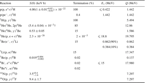
Table 2 shows the current best estimates for the astrophysicalS-factors.
Table 2.The solar fusion reactions. AstrophysicalS-factors for the solar pp chains and CNO cycle (adapted from [5]), percentage of the chain terminations (i.e. per4He nucleus produced via the
respective cycle) in which the respective reaction is involved, neutrino energy, and contributionQ to the solar energy generation of 26.7 MeV per4He nucleus produced [15].
Reaction S(0) (keV b) Termination (%) Eν(MeV) Q(MeV) p(p,e+ν)2H 4.00(1±0.01+0.02 −0.01)×10−22 100 0.422 1.442 p(pe−, ν)2H 0.4 1.442 1.442 2H(p, γ )3He 100 5.494 3He(3He,2p)4He (5.4±0.04)×10−3† 85 12.86 3He(4He, γ )7Be 0.53±0.05 15 1.586 3He(p,e +ν)4He 2.3×10⁻²⁰ 2×10⁻⁵ 18.8 19.795 7Be(e−, ν)7Li 15 0.862(90%) 0.862 0.384(10%) 0.384 7Li(p, α)4He 15 17.347 7Be(p, γ )8B 0.019+0.004 −0.002 0.02 0.137 8B( ,e+ν)8Be 0.02 15 17.980 8Be( , α)4He 0.02 14N(p, γ )15O 3.5+0.4 −1.6 7.297 16O(p, γ )17F 9.4±1.7 7.297
According to equation (7), apart from the astrophysicalS-factors, the reaction rates and thus also the individual neutrino branches depend on the local element densitiesnx. Particularly important in this context are the local densities of1H,3He, and4He. In the reference solar models, local equilibrium, corrected for element diffusion and gravitational settling of He towards the solar core, is assumed. This assumption has been validated in helioseismological measurements, whereas non-standard solar models7whichad hocintroduce strong mixing in the solar core to achieve non-equilibrium local element distributions [44] (mainly a local3He excess in the inner core in order to suppress the pp-II/pp-III chains; cf. figure 2) have been disproved. The same applies to models which assume rapid core rotation or strong trapped magnetic fields to counterbalance gravity, resulting in lower core temperatures and thus lower neutrino fluxes.
The neutrinos emitted in several steps of the pp cycle are referred to as pp, pep,7Be,8B, and hep neutrinos, according to the respective production reaction. Altogether 90% of the entire neutrino flux is believed to be pp neutrinos originating from the initiating reaction. They exhibit a continuous spectrum with an end-point of only 422 keV, which makes them the most difficult species to detect.
The second-largest contribution is7Be neutrinos from electron capture on7Be, the dom-inating process at the vertex of the pp-II and pp-III chain; cf. figure 2. As both the ground state and an excited nuclear level of the daughter nucleus7Li can be populated, the7Be-neutrino spectrum exhibits two discrete lines, at 862 keV (90%, ground state) and 384 keV (10%, excited level), respectively.
A line spectrum also characterizes pep neutrinos from the reaction p(e−p, ν)2H (not shown in figure 2(a)). The flux prediction for pep neutrinos is very accurate, as the process is closely linked to the pp reaction.
The opposite is the case for the high-energy8B neutrinos. Their prediction suffers from a large uncertainty in the astrophysicalS17(0)-factor [5]. There is an ongoing debate on the correct interpretation of experimental results from laboratory measurements ofS17and their low-energy extrapolation.
Not at all well determined, in addition, is the highest-energy neutrino branch: hep neutrinos from the pp-IV chain. The reason is the lack of low-energy measurements of the respectiveS -factor. Instead one has to inferS31(0)from measurements of thermal neutron capture on3He, a procedure which suffers from substantial uncertainties associated with the nuclear matrix elements involved. A recent assessment of the experimental and theoretical situation has revealed that even a factor-of-ten uncertainty for the flux prediction cannot be firmly rejected on the basis of the existing knowledge.
In contrast to the pp chains, the CNO cycle depicted in figure 3 is considered not to play a particularly prominent role for solar energy generation. It contributes only about 1.5% to the solar luminosity and 2% to the integral neutrino flux, according to solar model predictions8. From the reaction network, CNO-I dominates by far, and here it is the reaction14N(p, γ )15O which constitutes the bottleneck at solar temperatures. It is assumed that the CNO cycle has not yet reached equilibrium and14N is still being accumulated [35]. This leads to a higher flux of13N neutrinos, compared to the15O neutrino flux; cf. table 1.
As depicted in figure 2(b), CNO neutrinos exhibit continuous spectra, with typical energies
7 Almost all non-standard models were proposed in order to provide an ‘explanation’ of the observed solar neutrino
flux deficits. In order to reconcile solar neutrino fluxes being substantially lower than predicted by the reference models, they have to rely uponad hocassumptions for input parameters and/or physical processes which are not generally considered to correctly describe the Sun.
8 However, it is interesting to note that the CNO cycle would constitute the dominant process if the solar core
Figure 3.The CNO cycle, which contributes about 1.5% to the energy release of the Sun, gives rise to the continuous spectra of13N and15O neutrinos.
in the7Be range. In addition, the integral CNO neutrino flux is not substantially lower than that of7Be neutrinos: d<(CNO) dE dE0.2 i=384,861 keV <i(7Be).
Compared to the effort invested in preciseS-factor determinations of pp-cycle reactions, cross-sections for the CNO reactions are much less accurately known [5]. However, the LUNA collaboration has upgraded the accelerator utilized at Gran Sasso Underground Laboratory to determine the 3He–3He cross-section [93] for investigating CNO reactions at stellar energies [95].
3.3. Uncertainties and accuracy of neutrino flux predictions
For the interpretation of solar neutrino experiments, precise and trustworthy flux predictions constitute an important prerequisite. This applies not only to the integral flux, but, in particular, also to the individual neutrino branches. In the following we will discuss the influence of uncertainties associated with the input parameters and idealized physical concepts of the solar models on the neutrino flux predictions.
3.3.1. Opacities. The radiative opacity coefficients, determining how efficiently photons can transport energy from the solar centre outwards to the surface, are important for computations of the radial temperature profile and thus the relative contributions of the four subchains of the pp cycle. It was found empirically [15, 34] that the flux of7Be neutrinos,<(7Be), scales approximately asT8
c. Not surprisingly, boron neutrinos are even more sensitive,<(8B)∝Tc18,
whereas pp neutrinos, due to the luminosity constraint, remain essentially unaffected by variations of the core temperatureTc.
On the basis of improved determinations of the photospheric abundances of several elements [78], the OPAL opacity tables were updated in 1996 [101]. As for the intermediate region of the Sun, high-precision helioseismological observations have meanwhile allowed the probing of the influence on the speed of sound caused by changes of the opacity coefficients
exceeding a few per cent; the excellent agreement between the predicted and measuredcs -profiles supports the updated opacities. Neutrino flux predictions, except to some extent the highly temperature-dependent 8B and hep fluxes, can be considered robust with respect to opacity uncertainties.
3.3.2. Nuclear cross-sections and atomic screening. As already mentioned above, uncertainties associated with nuclear cross-sections arise mainly from two sources:
• Laboratory measurements are—except for the3He–3He reaction—performed in an energy range which is typically one order of magnitude higher than the Gamow region for the respective reaction in the solar core. Extrapolations of the data to solar energies introduce an uncertainty. The uncertainty is particularly serious for the7Be–p reaction, i.e.S17(0), giving rise to the8B neutrinos. Low-energy data forS17are entirely lacking, direct laboratory measurements suffer from a resonance at 0.6 MeV, and results from an indirect method exploiting Coulomb dissociation of8B in the strong Coulomb field of a Pb nucleus [112] which does not suffer from the resonance are only in marginal agreement with the direct measurements. In addition, the assessment of systematics in the S17-measurements has recently been criticized, which, if the criticism is justified, could indicate a need to increase the uncertainty ofS17 with respect to the published values [11, 95]. According to the empirical scaling law<(8B)∝S
17S340.81S33−0.4[15], this would reduce the accuracy of the flux prediction for8B neutrinos.
• Screening corrections become increasingly important at low energy. As mentioned above, the cross-section determined in laboratory experiments is enhanced by a factor
fe(E) >1 with respect to the bare-nucleus cross-section, due to the presence of bound atomic electrons. After several years’ controversy, the problem of reliably calculating these enhancement factorsfe(E)seems to be now largely dealt with, at least for atomic targets [5, 94, 104]. A reliable assessment of atomic screening is particularly important for the determinations ofS33, as the LUNA measurements extend down to 16.5 keV [29], corresponding to the lower edge of the Gamow peak.
3.3.3. Plasma screening. Electron screening in the solar plasma enhances the fusion rates by diminishing the effective repulsive Coulomb barrier with respect to bare nuclei [125]. The reference solar models employ a modified Debye–H¨uckel description to account for this [80,81,92]. There has been an extensive debate on the correct description for solar plasma screening, i.e. whether classical weak screening, intermediate screening [77], or dynamical screening is more appropriate (cf. [5, 35, 137] and references therein). More recent theoretical investigations seem to largely tend towards weak screening [5]. In summary, however, we do not consider the treatment of plasma screening to introduce a non-negligible uncertainty for neutrino flux predictions, except perhaps for the high-energy8B-neutrino branch.
3.3.4. Other sources of uncertainty. Other input to the calculations comprises the more or less idealized descriptions of physical processes considered relevant for the Sun—or their omission. For these issues also, new determinations of photosphere element abundances and the precision measurements of helioseismology have served to clarify the scenario.
Helium and heavy-element diffusion, i.e. gravitational settling towards the solar centre, has been proven to be non-negligible and is now generally taken into account in the reference solar models. The inclusion of diffusion has an effect on neutrino flux predictions, mainly for the high-energy8B neutrinos.
The sensitivity of solarp-mode frequencies on the equation of state leads to the conclusion that the appropriate prescription for the solar plasma is reasonably well understood and that associated uncertainties are under control.
Numerics could be important as regards interpolations of the tabulated radiative opacities and the numerical treatment of convection in the outer regions of the Sun, as both influence the solar temperature profile. However, Schlattlet al[127, 128] have constructed a solar model with an improved numerical treatment and found their results to agree with the reference models. We therefore do not consider this issue to introduce any non-negligible systematics for the flux predictions.
In conclusion, there remain two main sources for uncertainties in neutrino flux predictions. Firstly, though helioseismology has led to major improvements, it is still desirable to have more accurate radiative opacities. Secondly, several of the nuclear reaction cross-sections need to be measured at energies as low as possible in order to arrive at more reliable values for the astrophysicalS-factors. In particular, the knowledge of the cross-section factors forS17,S34, andS31needs to be improved. In parallel to low-energy measurements along the LUNA lines, a better theoretical understanding of screening effects in both the laboratory reactions and the solar plasma is desirable.
4. Solar neutrino detection
In this section we describe general principles for the detection of solar neutrinos. The absorption or scattering processes of neutrinos with matter via weak interaction in the relevant energy range are discussed and numerical values for the cross-sections are given. We emphasize the importance of charged-current (cc) as well as neutral-current (nc) interaction for the measurement of the flavour content of solar neutrinos. In addition, we discuss the basic technical items which are indispensable to the feasibility of solar neutrino experiments, emphasizing the important issue of background suppression. In section 4.4, operating experiments and their results will be presented, whereas the potential for upcoming projects to pinpoint neutrino masses and mixing angles will be discussed in section 6.
4.1. Charged-current and neutral-current detection
Weak interaction is mediated by exchange of either charged W±or neutral Z0bosons. These cases are referred to as charged-current (cc) and neutral-current (nc) interaction, respectively. Charged-current reactions of neutrinosνl(l=e, µ, τ) with nuclei can be described as ‘inverse beta decays’ of the form
νl+AZX→l−+AZ+1Y
where the nuclei X and Y have equal atomic numberA, but differ in their electric chargeZby one unit. The energy thresholdQis given byQ=mY+ml−mXfor ground-state transitions, wheremi(i=l,X,Y) are the masses of the particles involved in the inverse beta decay and a possible neutrino mass is neglected. In transitions to excited states, the additional energy has to be taken into account. For electron neutrinosνe, allowed reactions withQ-values in the MeV range and even below exist. Since the maximum energy of solar neutrinosEmax
ν ≈15 MeV,
detection of solarνewith nuclear targets using charged-current interaction is possible. One example is71Ga +ν
e →71Ge + e−which is used in the radiochemical gallium experiments GALLEX/GNO [67, 71] and SAGE [3] with a threshold of 233 keV; cf. section 4.4.
If the flavour of solar neutrinos is changed during their journey from the interior of the Sun to the Earth, for example due to oscillations as described in section 2, the detection of
those new flavours by the reaction above is forbidden kinematically. The reason for this is the large masses of the corresponding charged leptons,mµ=106.95 MeV andmτ =1777 MeV, which exceedEmax
ν by far.
However, neutral-current interaction is possible for all neutrino flavours. Hence, com-parison of observed rates in neutral-current as well as charged-current reactions allows one in principle to measure the flavour content of solar neutrinos arriving at the Earth and to determine whether neutrino oscillations do occur or not in the respective energy range. This is the aim of experiments which started data taking recently or are projected for the near future.
Neutral-current interaction contributes to elastic neutrino–electron scattering:
ν+ e−→ν+ e−
which is used in the SUPERKAMIOKANDE [133] and SNO [50] experiments for the detection of highly energetic8B neutrinos. The same reaction will be used in the future BOREXINO project [31] to examine the monoenergetic7Be neutrino flux atE
ν=861 keV.
The scattering ofνe is due to both cc and nc interaction, whereas theνµ,τ scatter only via the nc reaction. Hence, if the flavour of solar7Be neutrinos was converted almost totally fromνetoνµ orντ when arriving at the Earth, the counting rate in BOREXINO would be reduced by a factor of≈4, but still remain observable. In contrast, asνµ andντ produced by oscillations from solarνecannot interact via the cc reaction, for strongly converted7Be neutrinos the capture rate on nuclei would be suppressed dramatically. Inverse beta decays with such lowQ-values, apart from those of71Ga and37Cl, are known [118] and it is the aim of LENS [107] (cf. section 6.5) to perform a cc measurement which is—in contrast to the radiochemical gallium experiments—energy dispersive.
Another example of nc reactions used in solar neutrino experiments is the dissociation of deuterium,ν+2H→ν+ p + n, which occurs at a threshold of 2.2 MeV. This reaction is used in the SNO experiment [50] to investigate possible flavour conversion of solar8B neutrinos by comparing the measured counting rate with that of the cc reactionνe+2H→e−+ p + p.
Both examples show an experimental attempt by comparing cc and nc reactions to measure the flavour content of solar neutrinos arriving at the Earth. If these experiments show a significant deviation from a pureνe-flux of solar neutrinos, the hypothesis of neutrino oscillation will be unequivocally proven. In addition, it will also be possible to examine fundamental neutrino properties connected with oscillations, namely the mass difference and the mixing amplitude involved. How these questions will be investigated experimentally is described in sections 5 and 6.
4.2. General detector requirements
As neutrino detection is always based on weak interaction, the detection cross-section in the energy range relevant for solar neutrinos is tiny. For instance, the numerical value for elastic neutrino–electron scattering isσ(νe,e−)9.5×10−45(Eν/MeV)cm2, which is≈20 orders of magnitude lower than typical cross-sections of electromagnetic scattering processes. These low values make solar neutrino detection very difficult and require large target masses to be utilized in order to obtain reasonable event rates. Experiments use detector masses from the ≈100 t mass range up to the kiloton scale.
Since cosmic radiation, in particular high-energy muons, can produce background events which are indistinguishable from neutrino signals, all solar neutrino experiments are located
deep underground. The main background sources due to cosmic muons originate from
spallation processes. High-energy muons may produce electromagnetic and hadronic showers, generating radioactive nuclei which may mimic neutrino signals in the detector. The typical
reduction factors of muon fluxes achieved in underground laboratories are in the range of≈106 for a rock overburden of≈3000 m.w.e. (metres of water equivalent).
In addition, particle and gamma radiation is present due to ubiquitous natural radio-activity contaminants such as238U,232Th, and40K. Due to their high mobility, the noble gases 222Rn (produced in the decay series of 238U) and the anthropogenous fission product 85Kr (from atomic bomb tests) are jeopardizing particularly low-energy experiments. Hence, solar neutrino experiments usually have to be shielded against this radiation, and detector materials need to be selected carefully in terms of radiopurity.
4.3. Solar neutrino experiments: an overview
Solar neutrino detection is realized in two ways: either radiochemically or in energy-dispersive measurements. The former method is based on the chemical extraction of the small number of nuclei produced in inverse beta reactions during an exposure period of typically some weeks from a large amount of target (typically in the 100 ton range). After extraction, the back-decay of those nuclei is observed. This concept was realized for the first time in the Homestake37Cl experiment [49], which measures solar neutrinos via the reactionνe+37Cl → e−+37Ar at an energy threshold of 814 keV, giving access to the solar8B branch and, to some extent, to 7Be neutrinos. About twenty years later, the radiochemical GALLEX and SAGE experiments began to measure the integral flux of all solar neutrino branches using71Ga as target isotope. Here, the energy threshold is 233 keV, and for the first time pp neutrinos produced in the initiating solar fusion reaction p + p→νe+2H could be detected. Since 1998, GALLEX has continued as the Gallium Neutrino Observatory GNO.
Radiochemical experiments exhibit the potential to detect even the lowest-energy neutrino branch, pp neutrinos. The information on neutrino energy, however, is lost. Instead, a radio-chemical experiment constitutes something like a ‘fixed-threshold counting device’. Therefore, identification of the contribution of the individual neutrino branches to the detected signal cannot be accomplished in one single experiment alone, but requires information from several radiochemical detectors with different thresholds.
Direct information onEνis provided from energy-dispersive experiments. However, the energy threshold of the running and near-future projects is too high for assessing pp neutrinos. For the first time, the energy-dispersive technique was realized in the water Cherenkov detector KAMIOKANDE [91] and later in its upgrade SUPERKAMIOKANDE. The detection technique is elastic neutrino–electron scattering at an energy threshold of≈5 MeV (for SUPER-KAMIOKANDE), allowing only the high-energy part of the8B spectrum to be investigated. The reason for this high threshold is the formidable background from natural radioactivity arising in the≈MeV region.
The other operative energy-dispersive experiment, SNO, uses heavy water as target material. Its energy threshold is comparable to that of SUPERKAMIOKANDE.
A new detection concept, using large-volume, high-purity liquid scintillators for meas-urement of neutrino–electron scattering, allows investigation of neutrinos in the region around 1 MeV. This is possible due to the much higher light yield of scintillators, compared to that in the Cherenkov technique. The most advanced projects are BOREXINO and KAMLAND.
Table 3 lists running solar neutrino experiments as well as some projects which will start data taking in the future. Up to now, six different experiments have delivered data on solar neutrinos. Interestingly, in all cases, the measured flux is significantly lower than expected from solar model computations, establishing the so-called solar neutrino puzzle. In the following we will cover these experiments in detail and discuss the impact of their results on different solutions to the solar neutrino puzzle.
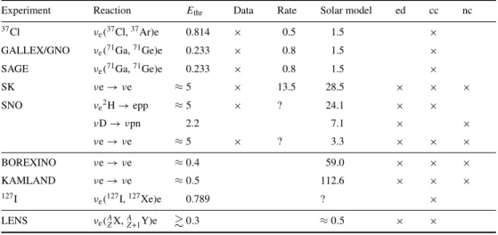
Table 3. A list of solar neutrino experiments according to their reaction mechanism, energy thresholdEthrin MeV, status (data available), measured counting rate in events per day, expected counting rates from the reference solar model (events/day), potential for energy-dispersive (ed), charged-current (cc), and neutral-current (nc) measurements. SUPERKAMIOKANDE (SK), SAGE, GNO, SNO, and the Cl experiment are taking data. BOREXINO, KAMLAND and the iodine experiment are under construction, LENS is a project still in an early development phase.
Experiment Reaction Ethr Data Rate Solar model ed cc nc
37Cl νe(37Cl,37Ar)e 0.814 × 0.5 1.5 ×
GALLEX/GNO νe(71Ga,71Ge)e 0.233 × 0.8 1.5 ×
SAGE νe(71Ga,71Ge)e 0.233 × 0.8 1.5 ×
SK νe→νe ≈5 × 13.5 28.5 × × ×
SNO νe2H→epp ≈5 × ? 24.1 × ×
νD→νpn 2.2 7.1 × × νe→νe ≈5 × ? 3.3 × × × BOREXINO νe→νe ≈0.4 59.0 × × × KAMLAND νe→νe ≈0.5 112.6 × × × 127I νe(127I,127Xe)e 0.789 ? × LENS νe(AZX,AZ+1Y)e 0.3 ≈0.5 × ×
4.4. Operating experiments and their results
4.4.1. Chlorine. For more than 20 years, the radiochemical37Cl detector operated since 1968 by Daviset al[48, 49] in the Homestake gold mine in Lead, South Dakota, USA, at a depth of 4200 m.w.e.9was the only active solar neutrino experiment. The experiment employs 615 tons of C2Cl4(37Cl natural abundance: 24.2%) as target material for the inverse beta-decay reaction37Cl +νe→37Ar + e−, which has an energy threshold of 814 keV. The experiment is mainly sensitive to8B neutrinos from the pp-III chain, and, to a smaller extent, to7Be and CNO neutrinos (cf. table 4).
Table 4. The spectral response of the chlorine experiment, according to the reference solar model [19]. The unit SNU (solar neutrino unit) is defined as 1 SNU = 1 neutrino capture reaction/1036target atoms s−1.
pp pep 7Be 8B 13N 15O Integral σ <ν(SNU) 0 0.2 1.15 5.9 0.1 0.4 7.7+1.2
−1.0
Only a fraction of ±0.2 SNU of the total error for the SNU prediction is associated with the neutrino capture cross-section which is dominated by a transition to an isobaric analogue state at 5 MeV and can be quite accurately determined from the beta decay of 37Ca. The dominant contribution to the error, in contrast, comes from the flux prediction of 8B neutrinos.
The few atoms of37Ar produced by neutrino interaction in the target of the Homestake experiment are extracted every few months by purging the target with helium, and added to the counting gas of a miniaturized, low-background proportional counter, where the electron capture (EC) decay of37Ar (half-life 35 d) is detected during a several-month counting period. 9 To allow a straightforward comparison of the shielding properties for different underground sites, the attenuation


![Table 1. Physical data and characteristics of the Sun. The upper group lists measured values acting as constraints for the reference solar models, whereas the lower group shows predictions from two prominent reference models, from [19] (BBP98) and [30] (BT](https://thumb-us.123doks.com/thumbv2/123dok_us/9949202.2889374/13.892.146.701.198.664/physical-characteristics-measured-constraints-reference-predictions-prominent-reference.webp)

![Figure 4. Angular distribution of the SUPERKAMIOKANDE solar neutrino data [135]. The data clearly point towards the Sun.](https://thumb-us.123doks.com/thumbv2/123dok_us/9949202.2889374/23.892.232.668.552.980/figure-angular-distribution-superkamiokande-solar-neutrino-clearly-point.webp)
![Table 5. The spectral response of the gallium solar neutrino experiments: predicted capture rates for the solar neutrino branches, according to the reference solar model [19], and capture cross-sections on 71 Ga [18].](https://thumb-us.123doks.com/thumbv2/123dok_us/9949202.2889374/25.892.234.514.801.992/spectral-response-neutrino-experiments-predicted-neutrino-according-reference.webp)
![Figure 6. Individual run results of the GALLEX and GNO solar neutrino experiments (method I) [73]](https://thumb-us.123doks.com/thumbv2/123dok_us/9949202.2889374/26.892.144.704.692.952/figure-individual-results-gallex-solar-neutrino-experiments-method.webp)
