Exploring the use of transformation group priors and the method
of maximum relative entropy for Bayesian glaciological inversions
Robert J. ARTHERN
Natural Environment Research Council, British Antarctic Survey, Cambridge, UK Correspondence: Robert J. Arthern <[email protected]>
ABSTRACT. Ice-sheet models can be used to forecast ice losses from Antarctica and Greenland, but to fully quantify the risks associated with sea-level rise, probabilistic forecasts are needed. These require estimates of the probability density function (PDF) for various model parameters (e.g. the basal drag coefficient and ice viscosity). To infer such parameters from satellite observations it is common to use inverse methods. Two related approaches are in use: (1) minimization of a cost function that describes the misfit to the observations, often accompanied by explicit or implicit regularization, or (2) use of Bayes’ theorem to update prior assumptions about the probability of parameters. Both approaches have much in common and questions of regularization often map onto implicit choices of prior probabilities that are made explicit in the Bayesian framework. In both approaches questions can arise that seem to demand subjective input. One way to specify prior PDFs more objectively is by deriving transformation group priors that are invariant to symmetries of the problem, and then maximizing relative entropy, subject to any additional constraints. Here we investigate the application of these methods to the derivation of priors for a Bayesian approach to an idealized glaciological inverse problem.
KEYWORDS: ice-sheet modelling
1. INTRODUCTION
One of the tasks presently facing glaciologists is to advise how the Greenland and Antarctic ice sheets might con-tribute to sea-level rise under the range of different climatic conditions that could occur in the future. To be genuinely useful to policymakers, planners of coastal infrastructure and other investors that are sensitive to future sea level, these glaciological forecasts will need to deliver information about the probability of the various possible outcomes that could be realized by the ice sheets. This makes it important to characterize the probability density function (PDF) of the sea-level contributions from Greenland and Antarctica.
Some estimates of how the climate of the atmosphere and oceans might evolve are available from general circulation models. These climate projections can be used to force dynamical models of the flow of an ice sheet, giving a forecast of the future contribution to sea level (e.g. Joughin and others, 2014; Cornford and others, 2015). At present these glaciological simulations are well adapted to investi-gating the sensitivity of the forecast to various perturbations in forcing, model parameters or initial conditions (e.g. Bindschadler and others, 2013). However, unless we can obtain reliable estimates of the probability of any particular perturbation actually occurring, the models cannot be used to evaluate the PDF of the contributions that ice from Greenland and Antarctica will make to sea level.
Glaciological forecasts over the next century or two will only be accurate if the models used to simulate the future begin in a state for which the geometry and flow speed are closely representative of the present-day ice sheets in Greenland and Antarctica. As in weather forecasting, the selection of the initial conditions for the simulation is an important component of the forecast. The procedure for setting up a model in a realistic starting state is known as initialization. One of the best ways to initialize large ice-sheet models is to use inverse methods (e.g. MacAyeal,
1992). These optimize the basal drag coefficient, viscosity or similar model parameters, to ensure that the model state from which the forecast proceeds agrees closely with a wide variety of measurements from satellites, aircraft and field campaigns. In this way the model starts from a state where the shape and flow speed of the ice accurately reflect what is happening now.
Ultimately, we are seeking to determine the complete PDF for the sea-level rise contribution from Greenland and Antarctica at times in the future that are relevant to planning decisions. Any errors in the initial conditions will propagate to give uncertainty in the simulation of future behavior. To quantify this uncertainty it is important to first characterize the uncertainty in the initial conditions in probabilistic terms. This makes a Bayesian approach to model initializ-ation attractive, since it offers a probabilistic interpretinitializ-ation, while allowing information from satellites and other obser-vational data to influence the joint PDF for viscosity, drag coefficient and other parameter values, as well as the initial values of state variables. Once this joint PDF has been obtained it can either be used to design ensembles for Monte Carlo experiments that evolve multiple simulations with a variety of initial conditions and parameter values, or as input to more formal probabilistic calculations that evaluate how uncertainty in the present state will propagate into the simulation used to forecast the future of the ice sheet. In this study we adopt a Bayesian approach to the problem of model initialization, and to the inversion of model parameters, such as the basal drag coefficient and viscosity.
A number of Bayesian inversions have been described previously by glaciologists (e.g. Berliner and others, 2008; Gudmundsson and Raymond, 2008; Raymond and Gud-mundsson, 2009; Tarasov and others, 2012; Petra and others, 2014; Zammit-Mangion and others, 2014). A key requirement in applying Bayesian methods is the definition
of a prior probability distribution for the parameters that we wish to identify. In this paper, our particular focus will be on how we can specify prior information for model parameters that we have very little useful information about. A good example is the basal drag coefficient. This can vary enormously, depending on details of the subglacial environ-ment that are completely unknown to us. The drag coefficient can be effectively zero for ice floating on water, but effectively infinite for ice frozen motionless to the bed. In many places in Greenland and Antarctica we do not know which condition applies. Furthermore, we do not know whether there are narrow water-filled channels, large water-filled cavities or broad sheets of water under the ice, so we cannot specify the length scale on which the basal drag coefficient might vary with any certainty. This makes it difficult to specify the prior PDF that is needed for any Bayesian inversion of this parameter.
One of our goals in this study is to reduce the subjectivity attached to glaciological forecasts. The general approach of defining the initial state of an ice-sheet model using inverse methods and then running the model forward in time to produce a forecast of the future might seem to provide a strategy for prediction that is physically based, mechanistic and largely free of subjectivity. By free of subjectivity we mean that different scientists should provide the same forecasts of the future behaviour of the ice sheet, assuming: (1) they are given the same set of observations; (2) they make the same rheological assumptions about the deformation of ice or sediment; and (3) they use the same conservation equations in the physical model that represents forces and mass fluxes within the ice sheet. However, even with observations, rheological assumptions and conservation equations in common, there is scope for making subjective decisions in the application of inverse methods that are used to identify parameters in the model, or the initial values for state variables. This applies particularly to the specification of the prior PDF for those parameters.
Subjective decisions made in defining the prior PDF will influence the initial state, and this, in turn, will affect the forecast of the ice sheet. The rate of ice flow into the ocean is sensitive to the basal drag coefficient and the ice viscosity (Schoof, 2007). Furthermore, the forecast of the ice sheet is typically obtained by solving a nonlinear system of equa-tions, and it may be quite sensitive to small changes in initial conditions or parameter values. Models that specify different prior PDFs for the spatial variations in viscosity and basal drag could potentially produce quite different projections of sea level.
The subjectivity attached to glaciological inverse meth-ods is not usually emphasized, and not much consideration has been given to whether it is important or not, so we consider it in some detail here. We do not claim to have a recipe to eliminate all subjective decisions from logical forecasts, nor is it our intention to criticize glacio-logical inversions that have relied upon them. There will always be decisions about which model to use, which datasets to include, which parameters to invert for and which methods to use to regularize the inversion. In common with many previous studies, our work has involved a variety of such decisions in mapping spatial patterns of basal drag and estimating the flow speeds within the Antarctic ice sheet (Arthern and others, 2015). The motiv-ation for the present study is to explore whether this approach can be improved upon by working within a
probabilistic framework. Tasked with providing probabilistic estimates of the contribution of the ice sheets to sea level, our goal is that those forecasts should be made as objectively as currently available techniques allow.
2. BAYESIAN INFERENCE OF MODEL PARAMETERS USING OBSERVATIONS
Suppose we are trying to estimate a vector,�, comprised of
Nparameters,�¼ ½�1,�2,. . .,�N�T, which may include the basal drag coefficient, �, at many different locations and viscosity, �, at many different points within the ice sheet. Bayes’ theorem provides a recipe for modifying a prior PDF for these parameters, pð�Þ, to include the information provided by new data, x¼ ½x1,x2,. . .,xM�T, which may include observations from satellites, aircraft, field parties or laboratory experiments. The result is the posterior PDF,
ppð�jxÞ ¼ plðxj�Þpð�Þ
pnðxÞ : ð1Þ
The prior pð�Þ is a PDF, defined such that pð�Þd� is the probability that the parameters lie within a vanishingly small ‘volume’ element d�¼d�1d�2. . .d�N, located at �, within
an N-dimensional parameter space, �, that includes all possible values of the parameters. The term prior reflects that this is the PDF before we have taken account of the information provided by the data. The information provided by the data,x, is encoded in the likelihood function,plðxj�Þ.
The likelihood function can be assumed known, provided two conditions are met. First, our physical model must be capable of estimating the measured quantities,x, if supplied with parameter values, �. Second, we must be able to estimate the PDF of residuals between these model-based estimates and the data,x(e.g. if model deficiencies can be neglected, this amounts to knowing the distribution of the observational errors). The likelihood function, plðxj�Þ, is then proportional to the PDF for observing the data,x, given that the parameters take particular values,�. The denomi-nator, pnðxÞ, is defined as pnðxÞ ¼R�plðxj�Þpð�Þd�, and
can simply be viewed as a normalizing constant, defined so the posterior PDF gives a total probability of R
�ppð�jxÞd�¼1, when integrated over all possible values
within the parameter space,�. To avoid ambiguity we will use subscripts to identify various different posterior PDFs (pp1,pp2, etc.), likelihoods (pl1,pl2, etc.), priors (p1,p2, etc.) and normalizing constants (pn1,pn2, etc.).
The notation for conditional probabilities,PðAjBÞ, denotes probability of event A given that B is true. The posterior,
ppð�jxÞ, is the PDF for the parameters,�, given that the data,
x, take the particular values observed. This means that, after we have taken account of all the information provided by the data, x, the posterior PDF, ppð�jxÞd�, gives the updated probability that the parameters lie within a small volume, d�, of parameter space located at�. Selecting the values of�that maximizeppð�jxÞprovides a Bayesian estimate for the most
likely value of the parameters.
The likelihood, function, plðxj�Þ, sometimes written Lð�;xÞ or Lð�Þ, can be considered as a function of � for the observed values of the data,x. It is sometimes the case when applying Bayes’ rule that the likelihood, Lð�Þ, is negligible except within a narrowly confined region of parameter space, while the prior, pð�Þ, describes a much broader distribution. This situation would indicate great
prior uncertainty in parameter values, �, but much less uncertainty once the information from the data is incorpor-ated using Bayes’ rule. In such cases, the information provided by the likelihood function,Lð�Þ, overwhelms the information provided by the prior,pð�Þ. Specifying the prior accurately in such circumstances is perhaps not so import-ant, since any sufficiently smooth function much broader than the likelihood function would produce a similar posterior PDF. However, we should not be complacent just because there are some circumstances in which it is not very important to specify the prior PDF accurately. There is no guarantee that this situation will correspond to glacio-logical inversions of the type that we are considering. Many aspects of the subglacial environment are barely con-strained by data, so it is in our interests to specify the prior PDF carefully.
In this paper we will apply two principles advocated by Jaynes (2003) to constrain the choice of prior PDF: (1) we will exploit symmetries of the ice-sheet model, by requiring that the prior PDF is invariant to a group of transformations that do not alter the mathematical specification of the inverse problem, and (2) using this invariant prior as a reference function, we will include additional constraints by seeking the PDF that maximizes the relative entropy subject to those constraints. Both approaches are described in detail by Jaynes (2003), and we will only make brief introductory remarks about them (Sections 5 and 6). Our intention is to guide, and as far as possible eliminate, the subjective decisions made during the inverse problem that defines the initial state of the model from the observations, particularly with respect to the choice of a prior PDF for the parameters. Although we concentrate here on methods advocated by Jaynes (2003), reviews by Kass and Wasserman (1996) and Berger (2006) provide a broader perspective and include additional background on the use of formal rules for the selection of prior PDFs.
3. THE CLOSE RELATIONSHIP BETWEEN THE PRIOR PDF AND THE REGULARIZATION OF INVERSE METHODS
Although we will use Bayesian methods, our investigation is relevant to a wide variety of glaciological inverse methods, many of which have been described in the literature without mention of Bayes’ theorem.
In particular, our approach is related to a broad class of inverse methods that minimize a cost function,Jmisfit, that
quantifies the misfit between the model and data. A common example is choosing model parameters that minimize the mismatch between model velocities,u, and observations of the ice velocity,u�, from satellites, so that the cost function is the unweighted sum of the squares of the misfit, e.g.Jmisfit¼ 12
P
i ui u�i �2
, or some similar function weighted by estimates of the observational error covariance,
R, e.g.Jmisfit¼1 2 P ij ui u�i � R 1 ij uj u�j � �
. Other cost func-tions to characterize the misfit between the model and the data have been proposed (Arthern and Gudmundsson, 2010; Morlighem and others, 2010) and the choice of cost function is therefore one way that subjective decisions can influence the inversion.
There are other aspects of the inversion that require subjective decisions. Generally speaking, simply minimiz-ing the mismatch with observations does not uniquely
define the spatially varying fields of basal drag and viscosity. This is because many different combinations of parameters allow the model to agree equally well with the available observational data. This is often dealt with by constraining parameters, using some kind of explicit or implicit regularization.
Regularization introduces additional information about parameters (e.g. requiring that they be close to some estim-ated value, or that they are small in magnitude, or that they vary smoothly in space). Before proceeding we will describe how regularization of inverse methods as commonly applied in glaciology relates to our Bayesian inversion.
The purpose of regularization is either to turn an ill-posed problem into a well-posed problem, or an ill-conditioned problem into a well-conditioned problem. As defined by Hadamard (1902), an ill-posed problem either has no solution, more than one solution, or a solution that varies discontinuously when small perturbations are made to any quantitative information provided (i.e. data). In any of these three cases it becomes impossible to precisely define a solution to the problem. On a practical level, especially when performing calculations numerically, we may come across problems that are not exactly ill-posed in the above sense, but are ill-conditioned. This means that a unique solution exists, but small changes to the data from measure-ment errors or numerical roundoff can result in large changes to that solution. If the resulting loss of precision is too great, we may be willing to constrain the solution in some other way, by regularizing the problem.
To be more concrete, we will give some simple examples of how a glaciological inversion can be posed or ill-conditioned, beginning with an example of a problem that does not have a unique solution. Suppose we would like to find the initial state for a model of ice of constant thickness flowing down a featureless inclined plane. Furthermore, suppose we know the ice thickness, the surface elevation and the flow speed at the surface (i.e. the data). Suppose now that we have no information about the drag coefficient at the base of the ice, or the ice viscosity, but wish to determine these using inverse methods.
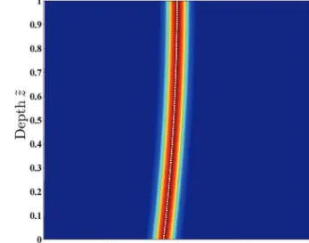
For a slab of the given thickness, the ice speed at the surface could be matched either by a rigid slab that is sliding at its base, or by a slab that is fixed at the base, but deforming through internal shearing (Fig. 1). None of the data provide information about the subsurface flow speed so we cannot distinguish between these two possibilities, or between these and some intermediate solution that is any combination of sliding and internal shearing that matches the specified surface velocity.
In practical applications, to avoid such non-uniqueness, it is rare that viscosity and basal drag are solved for simul-taneously. Rather, it is commonly assumed that one or other of these quantities is known perfectly. On floating ice shelves the viscosity is usually solved for on the assumption that basal drag is zero. By contrast, on grounded ice, the basal drag is usually solved for on the assumption that the viscosity perfectly obeys some rheological flow law with known parameters, so that the viscosity can be considered known.
The assumption that either the basal drag or the viscosity is perfectly known regularizes what would otherwise be an ill-posed problem, by avoiding a multiplicity of non-unique solutions. However, there are difficulties with this approach. First, for ice shelves where the bathymetry is poorly mapped, it may be difficult to be certain there is no basal
drag from some unidentified contact with the sea floor (Fürst and others, 2015). Second, on grounded ice, many factors that are not included in commonly used flow laws can affect the viscosity. These include such poorly known factors as impurity content, anisotropy, grain size, geothermal heating and damage from crevassing. This makes it problematic to assume we have perfect knowledge of the viscosity. Another consideration is that we have assumed in the problem specified above that the ice thickness is known perfectly. However the thickness is poorly known in many places, and it might be useful to invert for this field, rather than assume it is known perfectly (Raymond and Gudmundsson, 2009). Clearly, the problem of non-uniqueness would become even more acute if the observations of ice thickness were unavailable and we tried to solve for ice thickness as well as the basal drag and viscosity.
In the above example there are three parameters that we would like to invert for: ice thickness, ice viscosity and basal drag coefficient. Rather than assume we have perfect knowledge of two of these, it would be more realistic to acknowledge that there is considerable uncertainty in each, and to seek a compromise solution that jointly reflects these uncertainties.
For problems with many uncertain parameters a Bayesian approach is attractive. Rather than one set of parameters that minimize the cost function,Jmisfit, Bayesian inversion seeks the posterior joint PDF, ppð�jxÞ, for the parameters. This means that the combined uncertainty in basal drag co-efficient, viscosity and thickness can be evaluated. If we wish, we can later seek the values of the parameters that maximize the joint PDF, allowing us to solve simultaneously for the most likely values of all three quantities. To perform such Bayesian inversion we will need to define a prior PDF,
pð�Þ, for the parameters. It is this aspect that we concentrate on in this paper.
As an example of ill-conditioning, suppose the slipperi-ness at the base of the slab is not uniform as assumed above, but has fluctuations on some scale. As the characteristic size of these fluctuations decreases, their effect on the flow at the surface will diminish, until they become too small to have
any significant effect (Bahr and others, 1994; Gudmundsson, 2003). At the smallest scales their effect on the surface elevation and flow speed will be smaller than the accuracy with which these data are measured. Any inverse method that seeks to recover the fluctuations in basal drag on such a fine scale will be corrupted by the errors in surface elevation and surface velocity. In extreme cases, wild and unrealistic variations in basal drag might be introduced in an attempt to match the flow speed in the model to noise in the observations. This is known as overfitting. The usual remedy is to apply some form of regularization.
There are various different ways of regularizing inversions of basal drag to avoid overfitting, but a common approach is to enforce smoothness of the recovered pattern of basal drag. Many of the iterative algorithms that are used to minimize the cost function have a convenient property: they introduce features in basal drag on coarse scales in the first few iterations, then add progressively finer scales in later iterations (Maxwell and others, 2008; Habermann and others, 2012). Simply stopping after some number of iterations can prevent unrealistic fine-scale features being added. Deciding when to stop is a more vexing question, but there are criteria that can serve as a guide (Maxwell and others, 2008; Habermann and others, 2012). One remaining issue is that the regularized solution depends upon the initial guess for parameters used to start the very first iteration. Again, this is an opportunity for different people to make different choices.
A different form of regularization that is often used is Tikhonov regularization (e.g. Jay-Allemand and others, 2011; Gillet-Chaulet and others, 2012; Sergienko and Hindmarsh, 2013). Here the data–model misfit cost func-tion,Jmisfit, is replaced by Jtotal¼JmisfitþJreg, whereJreg is a term that penalizes solutions for the basal drag coefficient,
�, that are not smooth and promotes those that are. A common choice isJreg¼�reg
R
r�
j j2dS, for some constant
�reg, which adds a term proportional to the area integral of
the square of the magnitude of the horizontal gradient in basal drag coefficient (e.g. Sergienko and Hindmarsh, 2013). Adding this term to the data–model misfit cost function
Fig. 1.Simultaneous inversion for basal drag coefficient,�, and viscosity,�, is not well posed. Any observed surface velocity could be produced either by a well-lubricated base with high viscosity (left), or by a slab with high basal drag and low viscosity (right). Prior information about basal drag and/or viscosity is needed to determine which situation is more likely. The inversion may also be ill-conditioned if features at the bed are too small to affect the shape or flow speed of the upper surface. The usual remedy for non-uniqueness or ill-conditioning is to regularize the problem, and this can be interpreted in Bayesian terms as specifying prior probabilities for basal drag and viscosity. The coordinate axes used for the simple slab model are shown.
before minimization favors solutions for basal drag that have small gradients, hence the wildly fluctuating high-frequency oscillations that might otherwise be introduced by over-fitting are reduced.
When Tikhonov regularization is used, the value of�reg
can be varied to increase or decrease the strength of the regularization. It can be difficult to know what value to use for this parameter. Some heuristic conventions exist for selecting �reg, among them plotting the L-curve (e.g.
Jay-Allemand and others, 2011), or making use of a discrepancy principle (Maxwell and others, 2008), but in real applications these do not always provide an obvious choice (Vogel, 1996). It can also be difficult to know whether to penalize gradients in the drag parameter or its logarithm, i.e.
Jreg¼�reg
R
rln�
j j2dS. Other options include the square of basal drag, Jreg¼�reg
R
�
j j2dS, or its logarithm, Jreg¼
�reg
R ln�
j j2dS, but it is not always obvious why one should use one form rather than another, or even some combin-ation. It is clear there is scope for many different choices in applying Tikhonov regularization, and we have not even mentioned all of them.
Regularization requires the introduction of information that does not come from the observational data,x, that we have available from satellites, aircraft, field observations or laboratory experiments. This extra information must come from somewhere. The source of much of the subjectivity that we refer to in this paper is that the practitioners of the inverse methods often simply decide what seems reason-able. It is here that many of the subjective decisions that we would prefer to avoid can arise.
How smooth should the field of basal drag be? What should be the starting guess for iterative minimization of the cost function? What form of Tikhonov regularization should be used? How much can the viscosity vary from some prescribed approximation of the ice rheology, such as Glen’s flow law? Viewed from the Bayesian perspective, all of these decisions amount to the selection of priors for basal drag and viscosity.
One of the attractions of Bayes’ theorem is that it can provide the joint PDF for the parameters, given some observations with known error distribution. Crucially, the theorem cannot be applied without a prior for the par-ameters. This requirement to define a prior PDF for the parameters brings into the open many of the subjective decisions that are often made in an ad hoc fashion in the process of regularizing inversions.
As noted in many studies using Bayesian methods (e.g. Gudmundsson and Raymond, 2008; Petra and others, 2014), the link between regularization and specification of the prior can often be made explicit by taking the negative of the logarithm of Eqn (1),
lnppð�jxÞ ¼ lnplðxj�Þ lnpð�Þ þlnpnðxÞ: ð2Þ
Now, we identify a misfit function, Jmisfit¼ lnplðxj�Þ, defined as the negative of the log-likelihood, and a regularization term, Jreg¼ lnpð�Þ, that is the negative of the logarithm of the prior, andJ0¼lnpnðxÞ, which is just a constant offset for any given set of observations. Then it is clear that choosing parameters, �, that maximize the posterior PDF is the same as choosing them to minimize a misfit function, Jtotal¼JmisfitþJregþJ0¼ lnppð�jxÞ. The relationship,Jreg¼ lnpð�Þ, means for instance that quad-ratic regularization terms, such as Jreg¼�reg
R
r�
j j2dS,
correspond to specifying a Gaussian density function for
pð�Þ, such as expð �reg
R
r�
j j2dSÞ, and vice versa. From a Bayesian perspective the various options for Tikhonov regularization described above are just different ways of specifying a prior PDF for the parameters.
Working in the Bayesian framework provides some clarity to the definition of the cost function, Jmisfit, since it
suggests that if we want the most likely parameters we should use the negative log-likelihood function, lnplðxj�Þ,
to characterize the misfit with data, rather than unweighted least-squares or some other choice. It also clarifies the process of regularization, since it requires that the informa-tion to be added is explicitly formulated in terms of a prior PDF for the parameters. However, simply adopting the Bayesian approach does not tell us what the prior, pð�Þ, should be. So how should priors be defined for parameters that we have so little information about?
4. SUBJECTIVE PRIORS
One possible way to define a prior,pð�Þ, is to leave this up to the individual scientist performing the inversion. In the case of inverting for the basal drag under an ice sheet this seems a questionable choice. The posterior PDF, ppð�jxÞ, will be used to define the parameters for the model, and these parameters are an important component of the sea-level forecast. The glaciological forecast usually requires us to solve a nonlinear system of equations, which may be sensitive to small changes in parameter values or initial conditions, and we know that flow of ice into the ocean is sensitive to the basal drag coefficient and the ice viscosity (Schoof, 2007). This suggests that models that specify different prior PDFs for the spatial variations in basal drag could produce quite different projections of sea level. At present it is difficult to know how important this effect could be, but as more forecasts are produced, each with different models and different inversion methods, it will become easier to evaluate the degree of spread among projections.
Often a great deal of effort and cost is expended in developing the physical model, collecting the observations,
x, and characterizing the error covariance of those obser-vations. It seems questionable to apply such dedication to deriving the likelihood, plðxj�Þ, but then multiply this
function by a prior that is left up to individual choice, either through explicit definition of a subjective prior, or implicitly through choices of regularization strategy. This could be justified if the scientist performing the inversion has some real insight into the range of variation and the length scale on which basal drag varies. As mentioned above, there is great uncertainty regarding the subglacial environment and it is difficult to know how the insight needed to define the prior would be obtained. We emphasize that the prior,pð�Þ, is logically independent of the observations, x, that will be used in the inversion, so these observations cannot be used to provide insight into what the prior should be.
Another way of defining the prior, pð�Þ, would be to delegate the task to experts on the subglacial environment, asking them to define the prior for the basal drag, viscosity, etc. The justification for this would be that there are people who (without regard of the observations that we will use in the inversion) can provide us with useful information on the range of values that the viscosity and basal drag coefficient
can take, and the length scales they will vary over. If such experts exist then their views should be taken into account in definition of the prior,pð�Þ. However, it may be difficult to find anyone with such comprehensive information about the details of the subglacial environments of Greenland and Antarctica.
In the end, the main justifications for using subjective priors, or indeed heuristic approaches to regularization, may be (1) that they are easy to implement, (2) that it can plausibly be assumed, or checked after the fact, that the main results of the forecast are not too sensitive to the details of how this regularization is performed and (3) that it can be difficult to imagine what else could be done. The first point is certainly true, and should not be downplayed, since it allows large-scale calculations to be performed that could not be otherwise (e.g. Gillet-Chaulet and others, 2012; Morlighem and others, 2013; Joughin and others, 2014; Petra and others, 2014; Arthern and others, 2015; Cornford and others, 2015). The second point may well be true also, but seems to require that we address the third. After all, without first considering what else we might do to regularize the problem it is hard to argue that it won’t make much difference. In the following sections we outline two principles that have been advanced by Jaynes (2003) as a way of defining prior PDFs for parameters when minimal information about them is available.
5. TRANSFORMATION GROUP PRIORS
Transformation group priors use symmetries of the problem to constrain the function,pð�Þ, that is used as a prior PDF. In many mathematical problems knowledge of some particular symmetry can be extremely valuable, because it allows us to rule out a wide range of possible solutions that do not exhibit that symmetry. For instance, if there is some prior information available to us that can be written as mathemat-ical expressions involving�and if there are transformations that can be applied to these expressions that do not alter them in any way, then Jaynes (2003) argues that those transformations should also leave the prior, pð�Þ, un-changed. The motivation is to ensure consistency, so that for two problems where we have the same prior information we assign the same prior probabilities (Jaynes, 2003). Based on this, Jaynes (2003) argues that we should select priors that are invariant to a group of transformations that do not alter the specified problem. Surprisingly, in some cases, identifying the symmetries in the form of a group of transformations that leave the problem unchanged and then requiring that the function pð�Þ is invariant to those transformations can completely determine which function to use as a prior. The value of using transformation group priors is perhaps best appreciated by imagining that we use a prior that does not respect the symmetries of the specified problem. Then we would, in effect, be claiming access to additional information that is not inherent in the problem specification, and, if called upon, we should be able to provide a reasoned explanation of where that information has come from.
6. MAXIMIZING RELATIVE ENTROPY
In addition to the symmetries of the problem, we may have other information that is relevant to specification of the prior. Sometimes this information can be expressed in the
form of constraints that the PDF must satisfy. One common class of constraints are expectations of the form,
Z
�
pð�Þfið�Þd�¼Fi: ð3Þ For instance, if we have reason to believe that the expected value for the vector of parameters�is�, we would apply a constraint with fi ¼�, Fi ¼�. A similar constraint with
fi¼Fi¼1 requires that the PDF, pð�Þ, is normalized such that it integrates to one. Jaynes (2003) provides a recipe for incorporating such constraints, arguing that we should favor the PDF that maximizes the relative entropy subject to whatever constraints are imposed. The relative entropy of a PDF,pð�Þ, is a functional,HðpÞ, defined with respect to a reference PDF,�ð�Þ, as H¼ Z � pð�Þln pð�Þ �ð�Þ � � d�: ð4Þ
Multiple constraints of the form given by Eqn (3) can be imposed using Lagrange multipliers �¼ �1,�2,. . .,�Q
� �
, by seeking stationary points of the functional,
H1ðp,�Þ ¼ Z � pð�Þln pð�Þ �ð�Þ � � d�þ XQ i¼1 �i Z � pð�Þfið�Þd� Fi � � : ð5Þ
As described by Jaynes (2003), when the normalization constraint is enforced and other constraints,i¼1, 2,. . .,Q, are also imposed, stationary points ofH1ðp,�Þare provided
by PDFs of the form pð�Þ ¼ �ð�Þexp PQi¼1�ifið�Þ h i Z , ð6Þ Zð�Þ ¼ Z � �ð�Þexp X Q i¼1 �ifið�Þ " # d�, ð7Þ @lnZ @�i ¼ Z � pð�Þfið�Þd�¼Fi: ð8Þ Solving Eqn (8) often provides a convenient way of identifying values for the Lagrange multipliers,�, such that
H1is stationary and the constraints are enforced. Once these values of� have been obtained, Eqn (6) provides the PDF andZð�Þplays the role of a normalizing constant. If there are no constraints other than normalization, then finding stationary points of H1 results inpð�Þ ¼�ð�Þ. This means
that�ð�Þcan be viewed as a preliminary prior that will be modified, such that any additional constraints on pð�Þ are satisfied. Jaynes (2003) argues that the PDF, pð�Þ, that maximizesH, subject to whatever constraints are imposed has many attractive features. Roughly speaking, H can be viewed as quantifying the ‘uninformativeness’ of the PDF,
pð�Þ. MaximizingHis therefore a way of guarding against selecting a prior that is too prescriptive about which values of � are likely. This provides a safeguard against ruling things out that could possibly happen. A prior probability obtained in this way is guaranteed to satisfy the constraints, but is otherwise as uninformative as possible.
We would obviously prefer to have a very informative prior, since then we would know exactly which parameter values to use in our model. It may then seem strange that we are selecting the least informative prior possible, subject to the information introduced by the reference distribution and the constraints. The point is that we should only use an informative prior if we actually have the information to back
it up. Here, once we have defined a reference distribution, the extra information is being introduced in the form of constraints, or through the data that we will introduce later via Bayes’ theorem. For each constraint that we impose, the prior will become more informative, relative to the original PDF,�ð�Þ. If we were to subjectively choose a prior more informative than demanded by the constraints we would be guilty of subjectively introducing information into the in-version without good reason, and this is exactly what we are hoping to avoid, as far as possible. A prior that is too prescriptive about which parameter values are possible will only lead to overconfidence in the accuracy of our forecasts and to surprises when the forecast fails to deliver such accuracy.
It may seem that the problem has now simply changed from findingpð�Þto finding the preliminary prior,�ð�Þ. This is where a combination of the two approaches outlined above can be used. Jaynes (2003) suggests that invariance to a transformation group defining the symmetry of the specified problem should be used to define �ð�Þ. Having obtained �ð�Þ, any additional constraints can then be imposed by maximizing the relative entropy,H, subject to those constraints. This is the procedure that we will adopt in the rest of this paper.
7. APPLICATION TO A SIMPLE GLACIOLOGICAL PROBLEM
To introduce the methods outlined above, we will consider the simple problem of estimating the viscosity and basal drag coefficient for a slab of uniform thickness flowing down a plane. Although this is a highly simplified problem compared with the initialization of large-scale models of the Greenland and Antarctic ice sheets, it will turn out to contain many of the essential features of the more difficult three-dimensional problem, and therefore serves as a useful starting point to illustrate the methods.
We define a coordinate system in which thex- andy-axes are parallel to the planar bed of the ice sheet, which slopes downwards at an angle�below horizontal in the direction of increasingx, with no slope in the direction of increasingy
(Fig. 1). Thez-axis is taken to be normal to the bed, positive upwards, withz¼zbdefining the bed and z¼zsdefining the surface. The thickness,h¼zs zb, is assumed uniform,
and velocity in thex-direction,uðzÞ, is a function of depth. Any vertical shearing within the slab leads to a shear stress
�xz. The ice density,�, is assumed constant. The basal drag coefficient is�, and the viscosity within the slab is�, which is assumed constant with depth in this simplified problem. Within the slab, body forces from gravity are balanced by gradients in stress. At the lower boundary a linear sliding law is assumed, so the shear stress �xz¼�u. At the upper boundary the shear stress vanishes, so�xz¼0. For now, we will assume nothing about�or�, other than that they are positive constants.
For this simple system, conservation of momentum in the
x-direction gives the system of equations:
�@zu¼�xz, inzb<z<zs, @z�xz¼ �gsin�, inzb<z<zs,
�xz¼0, onz¼zs,
�xzþ�u¼0, onz¼zb,
ð9Þ
where g is acceleration due to gravity. Generally, before
performing an inversion using the model we will already have available a discrete version of the momentum equa-tions. For illustrative purposes we can consider a simple finite-difference discretization of the above system on a uniform grid that has n velocity levels at grid spacing
�¼h=ðn 1Þ and velocities in the x-direction of u1, u2, etc. These are defined on each of the different levels, sou1is the sliding velocity at the base andunis the flow velocity at the upper surface. We define
A¼XTDX, ð10Þ X¼ 1 1 1 : : : : 1 1 1 1 2 6 6 6 6 6 6 6 6 4 3 7 7 7 7 7 7 7 7 5 , f¼ 0 �gsin� : : �gsin� 0 2 6 6 6 6 6 6 6 6 4 3 7 7 7 7 7 7 7 7 5 , D¼ � � � �2 : : � �2 � �2 2 6 6 6 6 6 6 6 6 6 4 3 7 7 7 7 7 7 7 7 7 5 , u¼ u1 u2 : : un 2 un 1 un 2 6 6 6 6 6 6 6 6 6 6 6 4 3 7 7 7 7 7 7 7 7 7 7 7 5 : ð11Þ
The discretized system corresponding to Eqn (9) is then
Au¼f: ð12Þ
This is obviously a highly simplified model. We have only introduced it here so we have a very simple discrete system that we can use to illustrate how the methods can be applied in more general circumstances. More sophisticated ice-sheet models can be written in a very similar form, with A a symmetric positive-definite matrix,u a vector of velocities andfa vector comprised of body forces and forcing terms from boundary conditions.
If A and f are known, solving the system defined by Eqn (12) provides an estimate,A 1f, for the velocities,u. In
this paper we are not particularly interested in such a straightforward application of the model. Instead we would like to consider very general inferences about the velocity field,u, the forces,f, and the matrix, A, remembering that this matrix depends on the parameters,�and�, that we are trying to identify. We will also consider the possibility that the model is not perfect, so Eqn (12) is satisfied only approximately.
Note that in the above example, if we can estimate the matrix A, we can later derive the parameters � and � by computingD¼X TAX 1. To keep the following discussion
as generally applicable as possible, we will not yet assume any particular form for the system matrix,A, except that it is positive-definite and symmetric. Later, we will return to the problem with the particularAdefined by Eqn (10).
We will include in our vector of parameters,�, all of the quantities that we might perhaps want to estimate. These will include velocities, u, forces, f, the upper triangular (including leading diagonal) elements,Au, of the symmetric matrix, A, and the upper triangular (including leading diagonal) elements, Cu, of the model error covariance, C. Some of these would not usually be regarded as
‘parameters’, but we will continue to use this terminology for the unknown quantities that we would like to be able to estimate. We have only included the upper triangular elements of symmetric matrices in our list of parameters because the complete matrix, e.g. AðAuÞ, can always be recovered from these if needed.
For now, our only concern is to find a function that we can use as a prior for velocities,u, forces,f, and the upper triangular elements of A and C, based on what we know about the relationships between them.
It is important to recognize that we will not introduce any observations of any of the quantities until we have obtained the prior and are ready to include those observations using Bayes’ rule. Equally, once we have obtained a very general prior, we can later impose additional constraints on the form of the matrix, A. If expert knowledge or independent estimates of parameter values from laboratory experiments are available these can also be introduced later using Bayes’ theorem.
8. DERIVING A GENERAL PRIOR FOR DISCRETE SYMMETRIC POSITIVE-DEFINITE SYSTEMS
On the assumption that a symmetric positive-definite matrix,
A, exists that relates velocities,u, and body forces,f, with finite error covariance and finite bias, we have the following prior information: u A 1f¼�, Eu,fjA,C ��T � � ¼C, u,f2ún A,C2 PðnÞ: ð13Þ
Since we are assuming that the model has already been discretized using some particular set of basis functions, the velocities,u, and body forces,f, belong to the setúnof real vectors of known dimensionn. The matricesAandCbelong to the set PðnÞ of n�n real symmetric positive-definite matrices. The conditional expectation Eu,fjA,C ��T
� �
, is the average of��Tover the velocity, u, and body forces,f, for
particular values ofAandC. We will refer to the matrixCas the model error covariance. It is possible that the model is biased, so to be strict we should perhaps refer to this as the mean-squared error. It is defined as C¼Covð�Þ þbbT, whereb¼Eu,fjA,C½ �� is the expected bias of the model vel-ocities represented byA 1f, averaged over all possible for-cings,f, andCovð�Þ ¼Eu,fjA,C ð� bÞð� bÞT
h i
is the error covariance of the model, averaged over all possible forcings. Before looking at any data, we do not know anything aboutu,f,AorC, except for the information contained in Eqn (13). Before we can use Bayes’ theorem to make inferences aboutu,f,A andC from data, we need a prior PDF so that pð�Þd� is the prior probability that the parameters lie within a small interval, d�, of parameter space located at�. For our particular choice of parameters, this takes the form
pðu,f,Au,CuÞdudfdAudCu�
probability parameters lie within volume element dudfdAudCu f gatfu,f,Au,Cug, ð14Þ where du¼Qidui, df¼Qidfi, dAu¼ Q i,j�idAijand dCu¼ Q
i,j�idCij are the standard (i.e. Lebesgue) measures for
integration over elements ofu,f,AuandCu, the latter being the nðnþ1Þ=2 upper triangular elements of A and C, respectively. To label the domains of integration for u, f,
Au and Cu, we write U ¼fu2úng, F ¼ff2úng, Aþ¼ Au2únðnþ1Þ=2such thatAðAuÞ 2 PðnÞ � � , a n d Cþ¼ Cu2únðnþ1Þ=2such thatCðCuÞ 2 PðnÞ � � , and�¼ U � F � Aþ� Cþfor the parameter space that combines all ofU,F,
AþandCþ.
The information defined by the prior information (Eqn (13)) is invariant under several transformations:
T1ð Þ�: Orthogonal transformations, with � an n�n
orthogonal matrix, such that�T�¼��T¼I,
u7!�u, f7!�f, A7!�A�T, C7!�C�T: ð15Þ
T2ða,bÞ: Change of units. Rescaling bya>0 andb>0,
u7!au, f7!abf, A7!bA, C7!a2C: ð16Þ
T3ð Þr: Superposition of solutions,
u7!uþr, f7!fþAr,A7!A, C7!C: ð17Þ
T4(q): Switch velocities for forces and model for inverse. Repeatedqtimes, withq¼1 orq¼2,
u7!f, f7!u, A7!A 1, C7!ACA: ð18Þ
According to Jaynes (2003) it is important to specify the transformations as a mathematical group. Mathematically, a
groupis a set of elements (e.g.A,B,C, etc.) that also has an operation,�, that takes two elementsAandBof the set and relates them to a third elementP. To be a group the set and the operation must together satisfy certain conditions: (1) the operation must be closed so that the product, P¼A�B, always lies within the set; (2) the operation must be
associative, so that for any A, B and C in the set,
ðA�BÞ �C¼A� ðB�CÞ; (3) the set must contain an
identity element,I, such thatA�I¼A for any element A; (4) each element of the set must have aninverse,A 1, such
that A�A 1¼I. In Appendix A we show that the
transformations T1 to T4 satisfy these conditions individually and that their direct product defines a transformation group. As noted by Jaynes (2003), the key role played by the preliminary reference prior, �ðu,f,Au,CuÞ, is to define a volume measure for the parameter space,�. To qualify as a transformation group prior, this volume measure must be invariant to the group of transformations that do not alter the mathematical specification of the problem, but it need not correspond to the Lebesgue volume measure, dV¼
dudfdAudCu, that would apply if the parameter space
had a standard Euclidean geometry. The following distance metric is invariant under the group of transformations defined above:
ds2¼Tr�A 1dA A 1dA�þTr�C 1dC C 1dC�
þduTC 1duþdfTðACAÞ 1df, ð19Þ where Tr indicates the trace, obtained by summing elements on the main diagonal. We have written dA, dC, duand dfto represent infinitesimal changes to A, C, u and f. The invariance of ds2to the transformation group can be shown
by applying the transformations to Eqn (19), and using the invariance of Tr�A 1dA A 1dA�to inversionA7!A 1, scale changes A7!bA, and to congruent transformations of the form A7!BABT, where B is an invertible n�n matrix
From expressions given by Moakher and Zéraï (2011), the volume element that corresponds to the distance metric, ds2, is
dV¼2nðn 1Þ=2jCAj ðnþ3Þ=2dudfdAudCu, ð20Þ
where du, df, dAu and dCu are the usual Lebesgue measures. The following transformation group prior is therefore a suitable preliminary prior for derivation of a maximum-entropy PDF,
�ðu,f,Au,CuÞdudfdAudCu¼
Z012nðn 1Þ=2jCAj ðnþ3Þ=2dudfdAudCu, ð21Þ where Z0 is a non-dimensional constant that will be
determined by normalization.
Because the matricesAandCare defined to be positive-definite, the function �ðu,f,Au,CuÞ is finite everywhere within the parameter space,�, provided that Z0 is finite. However,�ðu,f,Au,CuÞis an ‘improper’ prior, as described
by Jaynes (2003). This means that if we attempt to integrate Eqn (20) over the parameter space, �, we find that this integral does not exist. Therefore a finite Z0 cannot be defined such that the prior,�ðu,f,Au,CuÞ, is a normalized
PDF over the entire parameter space, �. To allow us to interpret the function �ðu,f,Au,CuÞ as a PDF, we will consider a restricted section of parameter space, ��, for which the necessary integral exists, and for which there is a well-defined limiting process ��!� as �!0þ. For example, rather than an improper uniform prior for a single parameter over the interval ð 1,1Þ, a well-defined uniform prior can be defined over a range½ l=�,l=��, with
la constant that is finite and positive. Restricted domainsU�,
F�, Aþ� and C
þ
� that are subsets of U, F, A
þ
and Cþ, respectively, are defined in Appendix B. The restricted parameter space is then derived from the Cartesian product,
��¼ U�� F�� Aþ� � C
þ
�. Later, having derived a posterior PDF that depends upon�, we can investigate its behavior in the limit�!0þ. In Appendix B, we also define a separate non-dimensional parameter, �, that controls the smallest diagonal entries of positive-definite matrices.
Having defined the restricted parameter space, ��, we can seek the PDF,pðu,f,Au,CuÞ, that maximizes the relative entropy,H, HðpÞ � Z �� pðu,f,Au,CuÞln pðu,f,A u,CuÞ �ðu,f,Au,CuÞ � � dudfdAudCu, ð22Þ
subject to whatever constraints are imposed. In our case the constraints are that the PDF must be normalized, so that
Z
��
pðu,f,Au,CuÞdudfdAudCu¼1, ð23Þ
and that the conditional expectation of the error covariance, Eu,fjA,C ðu A 1fÞðu A 1fÞT
h i
is equal to C. Using the product rule, PðAjBÞPðBÞ ¼PðA,BÞ, for conditional prob-abilities of eventsAandBgives
pðu,fjAu,CuÞ ¼pðu,f,Au,CuÞ=pn2ðAu,CuÞ, pn2ðAu,CuÞ ¼ Z U�F� pðu,f,Au,CuÞdudf: ð24Þ The constraint, Eu,fjA,C ðu A 1fÞðu A 1fÞT h i ¼C, takes the form Z U�F� pðu,fjAu,CuÞ u A 1f� u A 1f�T C h i dudf¼0: ð25Þ
The constraints can be imposed using Lagrange multi-pliers, �1, a scalar, and �2ðAu,CuÞ, a positive-definite
symmetric matrix. We seek stationary points for the following quantity: H2ðp,�1,�2Þ � Z �� pðu,f,Au,CuÞln pðu,f,A u,CuÞ �ðu,f,Au,CuÞ � � dudfdAudCu þ�1 Z �� pðu,f,Au,CuÞdudfdAudCu 1 � � Z Aþ �C þ � Tr �2 Z U�F� pðu,fjAu,CuÞ � � ðu A 1fÞðu A 1fÞTdudf C i� dAudCu: ð26Þ
Whereverpn2ðAu,CuÞdoes not vanish, we can define Z1¼exp 1½ �1�,
�ðAu,CuÞ ¼�2ðAu,CuÞ=pn2ðAu,CuÞ:
ð27Þ
ThenH2 is stationary for PDFs of the form
pðu,f,Au,CuÞ ¼Z11�ðu,f,Au,CuÞe Trf�½ðu A1fÞðu A1fÞT C�g:
ð28Þ
The normalization constraint is satisfied for
Z1ð Þ ¼�
Z
��
�ðu,f,Au,CuÞe Trf�½ðu A1fÞðu A1fÞT C�gdudfdAudCu,
ð29Þ
in which Z1 is regarded as a functional of �ðAu,CuÞ. To evaluate the function� we require that the first variation of
Z1ð�Þ with respect to � is zero. This is analogous to identifying values for Lagrange multipliers by solving Eqn (8). Since the preliminary prior, �ðu,f,Au,CuÞ, is independent of u, carrying out an integration over U
provides the approximation
Z1ð Þ ¼� �n2 Z F�Aþ�C þ � �ðu,f,Au,CuÞj j� 12eTr½�C�dfdAudCuþE:E:, ð30Þ
where�written without arguments represents the constant, and E.E. represents edge effects arising because we have integrated overUrather thanU�. Here we neglect these edge effects, in anticipation that they become unimportant in the limit�!0þ, whereuponU
�! U. Then, requiring that the first variation ofZ1ð�Þwith respect to� is zero provides
�Z1ð Þ ¼� �n2 Z F�Aþ�C þ � �ðu,f,Au,CuÞj j� 12eTr½�C��� C 1 2� 1 � � dfdAudCu ¼0: ð31Þ
Since this must be true for any ��, and the quantities preceding�� in the integrand are all positive, applying the