Journal of
Economics and Political Economy
www.kspjournals.org
Volume 3 September 2016 Issue 3
Nonlinearities in Inflation and Growth Nexus:
The Case of Tanzania
By
Manamba EPAPHRA
†aaAbstract. Achieving high economic growth rate while maintaining low inflation rate, has become the main objective of monetary authorities all over the world. Indeed, empirical literature reflects that high inflation rates are detrimental to long run growth and entail welfare costs. To achieve this objective, central banks have availed different options from time to time which include inflation targeting. Monetary authorities in Tanzania have been targeting an inflation level of around 5 percent per annum for economic policy purposes. However, when high inflation is to be controlled, tight monetary policy is put in place which might in turn affect the economic activity. Also, the Tobin effect suggests that inflation causes individuals to substitute out of money and into interest earning assets, which leads to greater capital intensity which in turn promotes economic growth. Against these major points, this paper examines a non linear relationship between inflation and economic growth using both a quadratic and threshold endogenous models and attempts to identify the existence of threshold effects between these variables. The paper uses a data set spanning from 1967 to 2015. The most interesting finding of the estimations is that the estimated coefficient of the linear term of inflation is negative while the estimated coefficient of the square term of inflation is positive, suggesting a U-shaped effect as opposed to inverse or inverted U-shaped relationship found in other countries by previous studies. These results suggest that the Tobin effect may be valid for high inflation, in which people strongly realize the importance of substituting money for interest-bearing assets. This leads to an increase in capital investment, and in turn, an increase in economic growth even with high inflation rate. However, this U-shaped relationship between inflation and economic growth suggests that, the economy is better off at extremely low inflation episodes. The optimal inflation rate that ranges between 3.25 percent and 3.75 percent is obtained by minimizing the residual sum of squares and/or maximizing adjusted R-squared. These findings have some policy implications for the policymakers and development partners. The paper is consistent with policy suggestions by international agencies. Efforts to minimize inflation to a very low level are likely to have a positive effect on economic growth.
Keywords. Inflation; Economic growth; Threshold effects. JEL. E31, C13, 040.
1. Introduction
chieving sustainable economic growth and maintaining inflation rates within reasonable targets is central subject of macroeconomics policy. In fact, economists, policy makers and Central Banks across the world are concerned with high levels of prices and strive for achievement and maintenance of price stability. In Tanzania for example, the government through the monetary authorities institutes tight monetary and fiscal policies which often target the demand causes of inflation and therefore reduce inflation rate which in turn may
aa†
Department of Accounting and Finance, Institute of Accountancy Arusha, Tanzania. . +255 754399775
A
create an environment conducive to rapid economic growth (Fischer, 1993). Unsurprisingly, high inflation is believed to be detrimental to medium and long-run economic growth (Rutayasire, 2013) and therefore policy makers should aim for low rates of inflation (Seleteng, 2012).
The relationship between inflation and real economic growth however, is controversial in both theory and empirical findings. A study by Sidrauski (1967) suggests that there might no relationship between inflation and economic growth. Many countries have grown slowly despite low inflation (Fischer, 1983). In Neo Classical views, inflation increases economic growth by shifting the income distribution in favour of higher saving capitalists. This increases saving and thus economic growth. Also, according to Keynesians, inflation may increase growth by raising the rate of profit which in turn increases private investment. Indeed, Phillips (1958) hypothesizes that high inflation positively affects economic growth by lowering unemployment rates. In contrast, Barro (1995) points out that high inflation reduces the level of investment and a reduction in investment adversely affects economic growth. According to Gultekin (1983), economic growth rate depends positively on rate of return and that inflation reduces rate of return leading to low economic growth. Hence economic growth is negatively related to inflation. Many cross-country studies suggest the existence of an inverse relationship between inflation and economic growth and the magnitude of this relationship is envisaged to vary from region to region depending on the level of development and other factors (Seleteng, 2012). Many developed countries have mandate to keep inflation level within a particular target range because they have well-established and independent Central Banks (Seleteng, 2012). The main argument behind the negative relationship between the two variables is that businesses and households tend to perform poorly when inflation is high and unpredictable (Odhiambo, 2012). The different views about the relationship between inflation and economic growth imply that low inflation or macroeconomic stability is not a sufficient condition for sustained economic growth. Notwithstanding, the question about these variables is not only the simple relationship but also the level of inflation that can affect economic growth. According to Temple (2000), the existence and the nature of the relationship between inflation and economic growth is a subject of an extensive body of theoretical and empirical studies. Some studies use linear techniques and investigate the nature of the inflation-growth nexus (De Gregorio, 1993 and Fischer, 1993). Although many of these studies confirm the existence of negative relationship between inflation and economic growth, the causal relationship between them is a subject of controversy. For example, a study by Paul et al. (1997) suggests three different possibilities. One, they find no causal relationship between inflation and economic growth in 40 percent of the countries. Two, they find bidirectional causality in about 20 percent of countries and three, a unidirectional causality running either from inflation to economic growth or economic growth to inflation in the rest of the countries. Other studies use nonlinear techniques and argue that there exists a threshold or optimal level of inflation below which inflation may have no or even a positive effect on growth and above which inflation may be detrimental to economic growth. This threshold, however, differs from country to country and over time (Rutayisire, 2013; Salami & Kelikume, 2010; Singh, 2010; Sarel, 1996; Bruno & Easterly, 1998; Ghosh & Phillips, 1998; Khan & Senhadji, 2001; Moshiri & Sepehri, 2004; Mubarik, 2005; Lee & Wong, 2005; Drukker et al., 2005; Pollin & Zhu, 2006; Li, 2006; Hineline, 2007; Schiavo & Vaona, 2007; Quartey, 2010; Risso & Carrera, 2009; Ahmed & Mortaza, 2005). Nonlinearities of the relationship between inflation and economic growth also pose a question at what level of inflation that the relationship between the two variables will become negative.
Like many other countries, a central objective of macroeconomic policies in Tanzania is to achieve a high economic growth while maintaining a low inflation rate. Granted, Tanzania’s macroeconomic performance has improved substantially over the past 15 years with sustained high rates of economic growth and relatively low inflation (URT, 2015). During implementation of successful economic programmes, an inflation rate of 5 percent is used as a policy target. In fact, many sub-Saharan countries target inflation rate of around 5 percent (Table 1). Some economists however, believe that a low and stable inflation rate of 3 percent has a small cost in the economy (Mankiw, 2008). Also, an empirical study by Khan & Senhadji (2001) suggests that inflation threshold range is 1-3 percent for industrial countries and 11-12 percent for developing countries.
Table 1. Inflation Targets in Selected Sub-Saharan African Countries, 2016
Country Central Bank Target
Botswana Bank of Botswana 3.00 - 6.00 Percent
Ghana Bank of Ghana 8.00 +/-2.0 Percent
Kenya Central Bank of Kenya 5.00 +/-2.50 Percent
Malawi Reserve Bank of Malawi 14.2 Percent
Mozambique Bank of Mozambique 5.60 Percent
Nigeria Central Bank of Nigeria 6.00 - 9.00 Percent
South Africa South African Reserve Bank 3.00 - 6.0 Percent
Tanzania Bank of Tanzania 5.00 Percent
Uganda Bank of Uganda 5.00 +/-2.0 Percent
Zambia Bank of Zambia 7.00 Percent
Source: Central Bank News: Global Monetary Policy (2016)
In contrast, Kremer et al. (2009) suggest inflation thresholds of 2.5 percent and 17 percent for industrial and developing countries respectively. In a similar study, Pollin & Zhu (2005) estimate a threshold inflation range of 15-23 percent for low income countries.
Given the controversial relationship between inflation and economic growth and the belief that a particular threshold of inflation rates would have a positive impact on economic growth, the issue of inflation targeting as a monetary policy regime assumes even higher relevance in African countries as they attempt to reduce inflation to single digits in most countries, reduce fiscal and current account deficits, and contribute to improvement in the investment climate. However, the question raised is whether the inflation targets chosen for policy purposes optimal and consistent with economic growth. This problem can be well addressed by specific country study. Most of the studies conducted while aiming at estimating inflation threshold employ cross-sectional and panel data covering large sample of countries (Rutayisire, 2013). These studies are justified by their ability to generalize empirical findings and their policy implications appeal (Rutayisire, 2013). In fact, countries are heterogeneous (Lin & Ye, 2009 and Espinosa et al. 2010) and therefore, it is important to carry out country specific studies in order to relate findings to policy designs while allowing the incorporation of country specific characteristics (Rutayisire, 2013). Moreover, the current study is significant because even specific developing country studies suggest a wide range of inflation threshold levels ranging from 6 percent for Bangladesh (Ahmed & Mortaza, 2005) and India (Singh, 2010) to 22.2 percent for Ghana (Quartey, 2010). Specific country study thus, would in particular provide useful information about the appropriate location and width of inflation targeting band. This is also very important because in most developing countries, the Central Banks do not have a clear inflation targeting monetary policy framework.
The main objective of this paper is to investigate the nature of the relationship between inflation and economic growth in the context of Tanzania so as to better understand whether the country is striving towards goal of high growth and maintenance of price stability. In order to achieve this main objective, the paper is decomposed into two specific objectives. Firstly, to investigate the general relationship between inflation and economic growth and secondly, to investigate the nonlinearity of the inflation-growth nexus using time series data spanning from 1967 to 2015. In particular, the paper estimates the threshold or optimal level of inflation which is conducive for economic growth in Tanzania using a quadratic regression model which is estimated as a second-degree polynomial (Yabu & Kessy, 2015; Rutayisire, 2013; Pollin & Zhu, 2005; Clements et al., 2005; Devarajan et al., 1996; Hermes & Lensink, 2001 and Patillo et al., 2002) and threshold endogenous model used by Khan & Senhadji (2001), Chan & Tsay (1998), Hansen (1999; 2000) and Mubarik (2005).
2. Inflation Dynamics and Economic Growth in Tanzania
Inflation is one of the key determinants of economic performance, indicating growth, demand conditions, and the levels and trends in monetary and fiscal policy stance (Rutasitara, 2004). Thus, at all times, even when the rate of inflation seems to be low, authorities have to keep an eye on the different factors that may easily trigger a rise in inflation and erode the value of money holdings, trade flows, investor confidence, among others (Rutasitara, 2004).During the 1967-2015 period, the Tanzanian economy experienced mixed performance. Real GDP growth and inflation have been characterized by fluctuations, partly a result of economic policies pursued by Tanzania under a public sector-led economy embedded in the 1967 Arusha Declaration, and partly a result of exogenous factors, including deterioration in the terms of trade in the late 1970s and early 1980s, the collapse of the East African Community in 1977, and the war with Uganda’s Iddi Amin during 1978-79, the fall in the prices of exports such as sisal, tea and cotton, the rising price of imports such as oil crisis of 1973-1974, bad weather conditions and oscillating currency exchange rates. Growth of money supply also seems to contribute to fluctuations of the inflation during the period under study.
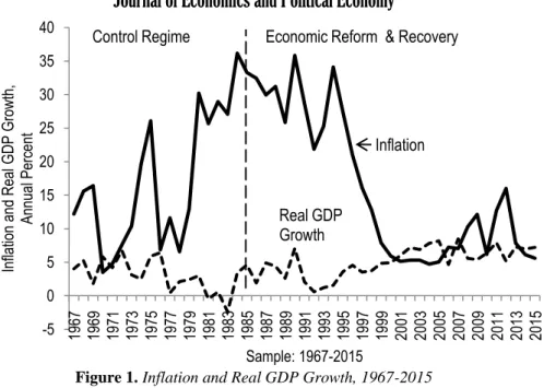
Figures 1 and 2 present the trends of inflation, real GDP growth and real per capita growth in Tanzania. The annual mean of inflation during the 1967-2015 was 16.5 percent while annual mean of real GDP growth and real per capita GDP growth were 4.3 percent and 1.4 percent respectively. In fact, Tanzania is among the least developed countries in the world with a 2014 per capita GDP of $588.3 measured at constant 2005 US$ (WDI, 2016).
Figure 1.Inflation and Real GDP Growth, 1967-2015
Figure 2. Real GDP Growth and Per capita GDP Growth, 1967-2015 Source: Author’s computation using data from World Bank WDI (2016)
The overall economic performance of Tanzania during the 1970s and first half of the 1980s was very disappointing. Deterioration in the economy revealed the inefficiencies of the state-dominated economy following the Arusha declaration of January 1967 that aimed at central planning and Government control. However, the fall of the economy in the early 1980s mainly was contributed to unsettled security and political conflict with Uganda and marked its lowest growth of -2.4 percent and per capita GDP of -5.3 percent in 1983 but the downfall of the economy in the early 1990s mainly was attributed to financial reforms and macroeconomic uncertainty such as high inflation rate. The real GDP growth rate during the 1970-1985 period, was 2.9 percent, while during the 1986-1995 and the 1996-2014 periods, real GDP rates were 3.1 percent and 6.1 percent respectively (World Bank, WDI, 2015). -5 0 5 10 15 20 25 30 35 40 1967 1969 1971 1973 1975 1977 1979 1981 1983 1985 1987 1989 1991 1993 1995 1997 1999 2001 2003 2005 2007 2009 2011 2013 2015 Inf lation an d Rea l GDP Gr owth, Ann ua l P er cen t Sample: 1967-2015 Inflation Real GDP Growth
Economic Reform & Recovery Control Regime
Tanzania adopted an economic reform programme in 1986 after experiencing a steady decline in economic growth in the late 1970s that led to a financial crisis in the early 1980s (Muganda, 2004). During that period, not only the Government owned and managed an important economic portfolio, but it also determined the prices of goods and services and established a large number of state enterprises with a view to creating public sector-led development framework. However, according to IMF, the approach produced adverse effects: it exacerbated distortions in the economy and led to a proliferation of parallel markets and unrecorded cross-border trade. Economic reforms allowed Tanzania not only to recover economic activity but also to operate a gradual transition from a state-controlled to a market-oriented economy relying on private sector. The reforms were implemented through successive economic and adjustment programmes as follows: Economic Recovery Programme (ERP) (1986-1989) and Economic and Social Action Programme (ESAP) or ERP II (1989-1992). However, before 1986, Tanzania implemented the National Economic Survival Programme (NESP) (1980-1985) and the Structural Adjustment Programme (SAP)(1983-1985). ERP I mainly focused on restoring external balance by pursuing prudent fiscal, monetary and trade policies and increasing in export earnings by an average of 16 per per annum over the programme period. It also focused on a progressive reduction in the rate of inflation to less than 10 percent by 1988/89 from over 33.3 percent in 1985, and achieving an average rate of economic growth of 4 percent 5 percent per annum, which would correspond to a positive growth in per capita income of 1.0 percent 2.0 percent. ERP II focused on the liberalization of the marketing of agricultural inputs and outputs, restructuring and privatization of the banking sector and allowing entrance of foreign banks and foreign exchange bureaus into the banking sector. It also concerned the restructuring and privatization of parastatals, civil service reform and further restructuring of markets for agricultural exports.
During the early period of reforms and recovery macroeconomic stability was not achieved mainly due to the government’s inability to control credit expansion to public enterprises, massive tax exemptions, poor revenue collections, and tax evasion. The large increase in tax exemptions was symptomatic of corruption and governance issues (Muganda, 2004).
During the late 1960s and 1990s inflation has always been a two-digit figure. Between 1972 and 1980 it fluctuated between 6 per cent and 30 per cent. At the end of the 1970s and the beginning of 1980, a radical increase was recorded. Inflation rose to 36.1 per cent in 1984 and 35.8 percent in 1990 from 3.4 percent in 1970. It stabilized at the level between 25 percent and 36 percent during the 1980-1996 period. This could be partly attributed to an expansion in the money supply, exacerbated by growing budget deficits. For example the growth rate of the money supply (M2) increased from 18.1 percent in 1981 to 41.8 percent in 1990 and 33.0 percent in 1995 (BOT, 2013).
The government of Tanzania's strategy for reducing inflation has, since 1986, focused on tight monetary policy and increased output production. This focus has been determined by the fact that Tanzania's inflation has been both a monetary and a structural phenomenon (Rutayisire, 1986). The task of slowing down inflation proved difficult. This difficulty was due to structural problems that hindered efficient production (for example, dependence on the weather) and inflationary financing of persistent fiscal deficits, caused by a combination of high government expenditure and poor domestic revenue collection (Solomon & de Wet, 2004). Inflation remained high on average during the 1986-1993 periods, although at a slightly lower level than the pre-reform level of 33.3 per cent in 1985. Over the past few years, inflation has stabilized at single digits, declining from an annual rate of 34 percent in 1994 to 5.6 percent in 2015 due to prudent monetary policy, a
favourable food situation and declining fuel prices (BoT, 2015). Also, export performance remained strong, driven by gold and tourism receipts (BoT, 2015). In fact, the significant decline in inflation rates in 1994 and the lowest inflation rates, ranging from 4.7 percent to 7.8 percent, achieved during the 1999-2007 reflects the impact of tight monetary and fiscal policies pursued by the central bank. Inflation averaged 7.7 percent during the 1999-2015 period, also buttressed by tight monetary policy and cash budgeting but increased to 16.1 in 2012, due to high world market prices for oil and food in 2012.
Over the period of last 15 years, both real GDP growth and real per capita GDP growth have been impressive. In particular, during the 2001-2015 real GDP growth and real per capita GDP growth averaged 6.7 percent and 3.9 percent respectively, underpinned by steady implementation of policy/structural reforms.
Along with economic reforms and recovery, priority spending aimed at promoting high economic growth and improving social services were channeled to investment in socio-economic sectors such as infrastructure, agriculture, health and education. As a result reforms were supported by large inflows of foreign aid and technical assistance. Table 2 reports economic growth and real per capita GDP and their determinants over the 1967-2015 period.
Table 2.Economic Indicators in Tanzania, 1967-2015
Indicator 1967-79 1980-89 1990-99 2000-09 2010-15
Real GDP growth rate 3.9 2.3 3.3 6.5 6.8
Real per capita GDP -0.7 -0.3 -0.3 3.9 3.4
Inflation rate 11.9 30.1 23.1 6.8 9.1
Trade, percent of GDP 43.4 24.6 35.2 17.0 51.2
Investment, percent of GDP 25.6 24.4 27.7 19.0 12.9
Population growth 3.1 3.1 3.0 2.9 3.2
M3 Growth, annual percent 20.6 24.1 27.1 22.0 16.2
Source: Author’s calculations using data from World Bank Development Indicators (2016)
During the 1980-89 period, overall investment declined significantly mainly due to immense difficulties with high inflation during the same period. This means that, it has been costly to hold wealth in terms of money because of negative real interest rates. This might be caused by national policies that discourage liberalization of economy where the government controlled the economy. During the entire period of 1990-99, the gross investment was on average 27.7 percent of GDP. Also, the removal of trade restrictions improved the openness of the economy and boosted the external sector. Table 1 suggests that, as a result of the implementation of sound economic policies, all the economic indicators performed better on average in the 1990-99 period than in the 1980-89 period.
Understandably, macroeconomic instability may adversely affect economic growth. For example, uncertainty related to higher volatility in inflation could discourage firms from investing in projects that have high returns, but also a higher inherent degree of risk. The usual arguments for lower and more stable inflation rates include reduced uncertainty in the economy and enhanced efficiency of the price mechanism. A reduction in the level of inflation could have an overall effect on the level of capital accumulation in cases of tax distortions or when investment decisions are made with a long-run perspective. However, evidence on the relationship between inflation and growth is somewhat mixed (Bassanini & Scarpetta, 2001). Although it is widely accepted that that investment and growth suffer in cases of high inflation, the relation is less clear in cases of moderate or low inflation (Edey, 1994; Bruno & Easterly, 1998). Indeed, Table 1 does not provide evidence that higher inflation correlates systematically with lower
economic growth or per capita GDP growth or the reverse. For example, as the Table depicts both inflation and real GDP growth increased on average from 6.8 percent and 6.5 percent in the 2000-09 period to 9.1 percent and 6.8 percent in the 2010-15 period respectively.
Table 3 also confirms the ambiguous relationship between inflation and economic growth. Following the approach by Yabu & Kessy (2015), Rutayisire (2013), Mubarik (2005) and Ghosh & Philips (1998), sub-ranges of inflation rates are computed and categorized in ascending order. Mean and median inflation and growth rates corresponding to each inflation range are also estimated. It is worth recalling that on average for the whole sample period, inflation rate ranges between 6.8 percent and 30.1 percent while economic growth varies between 2.3 percent and 6.8 percent (Table 2). Table 3 shows that, from the second to the sixth inflation ranges, a higher mean or median inflation rate is associated with a lower economic growth suggesting a negative relationship. However, the higher mean or median inflation rates corresponding to the second, seventh and eighth inflation ranges coexist with impressive mean or median economic growth rates. These observations provide some pre-evidence that there may be a non-linear relationship between the two variables.
For more precise picture, it is worthy to understand the historical nature of the relationship between inflation and growth through more visual examinations. Figures 3 and 4 present much the same information but for several different sub-samples and in graphical form. Figure 3 provides a more direct view of the association between inflation and growth association by plotting the mean GDP growth rate against the mean inflation rate for each of 8 subsamples defined according to degree of inflation. The key observation is that, first, at the very lowest inflation rates, inflation and growth are positively associated. Second, at inflation rates, say between 6 percent and 27 percent, the relationship is negative. Third, beyond inflation rate of say 27 percent, the relationship is again positive implying, plausibly, that an increase in inflation from 6 percent to 27 percent impairs growth more than an increase from 27 percent to 36 percent. In fact, the economic growth improves when inflation rates rise above 27 percent.
Table 3. Inflation Ranges and Economic Growth in Tanzania, 1967-2015
Number of Observations
Inflation GDP Growth
Inflation Band Mean Median Mean Median
All observations 49 16.5 12.8 4.3 4.6 1: t
0 5 3 5.9 4.8 4.3 5.8 2: 5
t 10 15 6.4 6.0 6.3 6.6 3: 10 t
15 8 11.9 12.2 4.1 3.4 4: 15
t 20 5 16.7 16.1 3.6 3.5 5: 20
t 25 2 21.4 21.4 2.6 2.6 6: 25 t
30 9 27.2 27.1 2.0 2.1 7: 30
t 35 5 32.2 32.4 3.1 3.0 8: 35 t
2 36.0 36.0 5.2 5.2Figure 3. Mean Inflation and Real GDP Growth, 1967-2015
Notes: Median inflation and growth rates in equal-sized subsamples, defined according to range of inflation
More systematic evidence for the past 49 years is given in Figure 4 and Table 5, which show the correlation between inflation and economic growth. Figure 4 presents the scatter plot for the whole sample. Generally, the bivariate evidence suggests a negative relationship between inflation and growth. This relationship appears to break down, however, somewhere in the inflation range between 20 and 30 percent; and beyond that level there is a positive relationship. This U-shaped relationship between inflation and economic growth observed using Tanzania data, however, is surprising but interesting. In fact, many studies on the non-linear effect of inflation on economic growth in other countries have proved existence of an inverted U-shaped relationship between the two variables.
Table 4 reports the correlation matrix for inflation and economic growth, in three sub-samples. A correlation-matrix with the inflation levels less than 10 percent shows a negative but weak correlation, suggesting that there is a possibility of positive correlation between the two variables in very low inflation levels that tend to partially offset the negative correlation as Figure 3 illustrates. The correlation-matrix with inflation levels between 10 and 24 percent shows a negative correlation between inflation and GDP growth while the correlation-matrix with inflation levels above 24 percent shows a positive correlation. Therefore, from the three correlation matrices, it can be assumed that the relationship between inflation and growth is non linear.
Figure 4. Scatter Plot: Inflation and Real GDP Growth, 1967-2015 Source: Author’s calculations using data from World Bank Development Indicators (2016)
Table 4. Correlation Matrix for Inflation and Economic Growth, in three Sub-Samples, 1967-2015 Inflation Less than 10 Percent
Inflation Growth Mean
Inflation 1 6.042
Economic Growth -0.095 1 6.228
Inflation Between 10 Percent and 24 Percent
Inflation Growth Mean
Inflation 1 14.940
Economic Growth -0.222 1 3.587
Inflation Above 24 Percent
Inflation Growth Mean
Inflation 1 29.878
Economic Growth 0.425 1 2.744
Source: Author’s computation Using Data from World Bank WDI (2016)
In fact, the positive relationship between inflation and economic growth is not surprising. The Tobin’s (1965) framework also reveals a positive relationship between inflation and growth. The Tobin effect suggests that inflation causes individuals to substitute out of money and into interest earning assets, which leads to greater capital intensity which in turn promotes economic growth.
3. Literature Review
3.1. Theoretical Literature Review
Economic theories such as Classical, Keynesian, Neo Keynesian, Monetarist, Neo-Classical and Endogenous growth theories have great contribution to the relationship between inflation and economic growth. However, these theories reach a variety of conclusions about the responsiveness of growth to inflation. This subsection discusses the contribution of each theory to the relationship between the two variables.
3.1.1. The Classical Growth Theory
Classical theory is the first modern school of economic thought. Indeed, Classical economists as chiefly represented by Adam Smith, David Ricardo, and Thomas Malthus laid the foundation for a number of growth theories. The foundation for Classical growth theory is laid by Adam Smith who posits a supply side driven model of growth, which emphasizes the need for incentives to save and invest if the economy is to grow, linking it to factors of production as follows:
K L N
fY , , (1)
where Y the level of output (supply)
K the stock of physical capital
L the labour force
Nland
Model (1) implies that supply is a function of capital, labour, and land. Consequently, output growth is driven by investment growth, population growth and land growth as well as the increase in the overall productivity. The theory assumes a self-reinforcing growth or increasing return to scale and that savings creates investment, hence growth. The link between inflation and growth of output is not specifically articulated in classical growth theories. However, the relationship between the two variables is implicitly suggested to be negative, as indicated by the reduction in firms’ profit levels through higher wage costs. Profit declines, not necessarily because of decreasing marginal product of labour, but because competition for labour drives wages up. The fall in the profit level
discourages the firms who are the source of wealth creation. Thus, the price increase will have a negative impact on productivity of the firms leading to decline in the level of the economic growth (Pentecost, 2000).
3.1.2. Neo-Classical Growth Theory
The neo-Classical growth model was developed primarily by Solow (1956). In the neoclassical growth model also known as exogenous growth model, the long-run growth rate is determined by the rate of population growth and technical progress which are assumed to be exogenous. The Solow model of production is expressed as
K L
Af Y , (2) where YReal GDP K Capital stock L Labour employment A Exogenously determined factor of technology and capital-to-GDP ratio can take on any nonnegative value, that is
0 Y K k (3)
Equation (2) can be written in growth terms as follows
A A L L K K Y Y 1 (4) ogress Technical Labour in Growth Labour of Share Capital in Growth Capital of Share Output of Growth Pr
where denotes share of capital in national product, 1denotes share of labour
in national product.
Technically the neoclassical production function is homogeneous of degree one and implies that factors must be available or else output will be zero, that is, economy does not exist. In the short-run, the model allows unlimited substitutability between capital and labour to produce any given amount of output, that is, any amount of capital can be used with the appropriate amount of labour basing on the law of diminishing return. While in the long-run, when economies of scale are being realized, both factors will be increasing proportionally, and eventually results in increasing returns to investment. The theory also assumes that the possibility of achieving high growth rates will be low when there is an increase in the average per capita income (Crafts & Toniolo, 1996). The justification is, the countries with low per capita income have a weak capital formation, and therefore, investment will achieve growing returns contrary to the countries with high per capita incomes (Tawiri, 2010). This leads to the conclusion that developing countries are able to converge in income with developed countries if they succeed in increasing domestic and foreign investment (Tawiri, 2010). However, this hypothesis has been successful in practice in developed countries, but has not achieved the same result in developing countries (Obstfeld, 2008) leading to the emergence of modern neoclassical economic theory which relies on the hypothesis of conditional convergence. The modern neo-classical theory isolates some variables that affect growth rate and per capita income, which lead to the proof of
the opposite relationship between growth and per capita income. The theory adds other variables such as, education and trade.
Neo classical economists give their own explanation about the relationship between inflation and economic growth. Mundell (1963) and Tobin (1965) explain the effect of inflation on economic growth based on neo-classical growth theory. They believe that increased nominal interest caused by inflation will make people option to investment instead of consumption. This will result in increasing capital accumulation which will stimulate economic growth. Mundell (1963) using the IS-LM curves finds a positive relationship between inflation and growth. He argues that an increase in inflation or inflation expectations leads to a decline in real money balances, which decreases the wealth of people. To accumulate the desired wealth, people save more by switching from holding money to assets, which increases the assets price, thus driving down the real interest rate. Greater savings leads to higher capital accumulation, which leads to rapid economic growth. Tobin (1965) also supports Mundell's idea that inflation is positively related to economic growth. Indeed, the Mudell-Tobin effect suggests that high rate of inflation permanently increases the levels of output. During high rates of inflation, people will tradeoff between holding money with acquiring more physical capital; as a result capital intensity will increase and in turn stimulate output growth. However, the Mundell and Tobin view of the positive relationship between inflation and economic growth has received challenges from various scholars.
Stockman (1981) develops a model that shows the negative effect of high inflation on steady state level of output and wealth. Stockman (1981) uses the cash in advance constraint model. The model suggests that inflation lowers the steady state capital stock. Stockman (1981) argues that because increase in inflation reduces the purchasing power of money balances, people tend to reduce holding money as well as purchase of capital goods, which in return lowers the steady state level of output. Like Stockman (1981), Lucas (1982) & Svensson (1985) use the cash in advance constraint model to explain the relationship between inflation and output. In the cash in advance model, money is demanded because it is the only means of purchasing goods. Specifically, Lucas (1982) argues that since consumers earn interest on deposits not cash balances they will prefer to have most of their money in deposits during inflation. However they will hold just enough cash to pay for their consumption. This will eventually lower asset purchases, which lower capital accumulation and hence reduce output growth. Similarly, Svensson (1985) points out that if cash is needed to finance consumption then high inflation will lead to less of the goods to be consumed because high inflation reduces the value of money. Therefore high inflation affects real variables such as consumption and output.
3.1.3 The Keynesian Theory
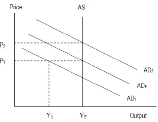
Keynesian theory does not assume that any supply will meet its demand if only prices are flexible enough. Instead, it argues that where constraints to expansion exist they are most likely to arise because the economic system is unable to generate sufficient demand to fully employ labour. Keynesians tend to attribute inflation more to demand pressures within an economy. Keynesians’ explanation of the long run economic growth path is implicitly captured in the business cycle concept (a short run phenomenon) developed within the aggregate demand (AD) and aggregate supply (AS) framework. According to the AD-AS framework, changes in the demand side of the economy affect both prices and output, arising from changes in expectations, labour force, fiscal and monetary policy, among others. In fact, Keynesians argue that there is a positive relationship between inflation and output, such that even if there is an increase in prices of goods in the economy, output would not decline because producers have to satisfy the demand
requirements of consumers. Figure 5 presents the AD-AS under the framework of Keynesianism. The framework shows the relationship between output, employment and inflation.
Figure 5. AD-AS Curve under the Framework of Keynesian
Source: Xiao (2009) with some modifications
When current resources are not fully utilized, promoting effective demand through interventions by governments will improve output and employment without generating inflation until output reaches its full production level, YF. YF is
determined by the long-run aggregate supply curve, AS. Promoting effective demand will shift the aggregate demand from AD1 to ADF, under which output is at
its full production level. Price will not increase until demand rises beyond ADF. If
equilibrium output demanded is more than full-employment output at initial price, P1, there will be excess demand in the economy and the price level will be bid up,
causing demand pull inflation.
The Keynesian theory also suggests that increase in money supply affects inflation through interest rate movements. In this view, money is considered a close substitute for a limited number of financial assets such as bonds, and thus an increase in money supply creates excess supply in the money market, leading to an increase in prices of financial assets and subsequent fall in the interest rate. This in turn, increases investment demand, depending on the interest rate sensitivity of the investment. An increase in investment leads to increased aggregate demand, thereby triggering inflationary pressures in the economy. This theoretical explanation may, however, only apply in the short run. A fall in the interest rate may stimulate increased investment, thereby aggregate demand and increased inflation in the short run. But, in the long run, increased inflation may cause output to contract thereby leading to the reduced demand for money in the economy. According to the money demand relationship the reduced demand for money would lead to a rise in the nominal interest rate in the long run.
3.1.4. The Monetarist Theory
Monetarism is very closely allied with the classical school of thought. It is essentially an extension of classical theory which is developed to explain stagnation and inflation problems. Monetarists argue that if the money supply rises faster than the rate of growth of real GDP then there will be inflation. If money supply increases in line with inflation then there will be no inflation. They argue that money is a close substitute for real assets such as houses and land, and financial assets such as bank deposits, treasury bills, and bonds and that any extra cash balances realized from the increase in money supply will be spent on those assets rather than held as idle money balances. This in turn leads to excess demand
for assets, which causes prices to rise. Monetarism argues that money supply is the only factor that determines price levels in an economy and the only intervention that a government can do is to manage the growth rate of money supply to harmonize it with the growth rate of real GDP in the long run. The two key areas of Monetarists are Quantity Theory of Money and Expectations-augmented Phillips Curve.
The Quantity Theory of Money which is a bit of Classical theory, based around the Fisher Equation of Exchange is expressed as
PT
MV (5)
where M total stock of money in an economy
V the velocity of circulation of that money
P the average price level
T the number of transactions taking place
Essentially the quantity theory of money is a hypothesis about the main cause of changes in the purchasing power of money. The theory suggests that changes in the value of money are determined mainly by changes in the quantity in circulation. When money becomes abundant, its purchasing power declines, and consequently the average of commodity prices increases. In contrast, if money becomes scarce, its purchasing power increases and commodity prices decline. In this view, the amount of money in circulation is the main determinant of the price level. It is, however, not easier to measure the number of transactions,T. It is, therefore, replaced byY. Thus PY is the nominal income or output where Y is the total income. Now the quantity theory equation becomes:MVPY.This is known as the income version of quantity theory of money. Monetarists believe that in the short term velocity, V,is fixed. This is because the rate at which money circulates is determined by institutional factors. They also believe that output, Y,is fixed. Therefore an increase in the money supply will lead to an increase in inflation. The Quantity Theory of Money can be transformed to depict an unambiguously negative relationship between inflation and economic growth as follows:
Y Y M M (6) where = Inflation M M
= The growth rate of money supply
Y Y
= The growth rate of output
The quantity theory version of the demand-pull inflation is also illustrated using LM curve as Figure 6 reports. Assuming the initial equilibrium value of real output is at full employment level of income, YF,that is shown by the intersection of IS and LM curve at e in Panel (A). Monetary policy increase in money supply will shift the LM curve rightward to LM1along the given IS curve.
Figure 6. Money Supply, Inflation and Income Source: Smriti Chand with some modifications
At the initial equilibrium level of income, this increase in money supply would push the interest rate down to R1 to maintain equilibrium in the moneymarket (Branson, 1979). This in turn will lead to an increase in equilibrium output demanded toY1,at the given price level, produce horizontal shifts in the economy’s demand curve. The position of the IS curve is unchanged because the aggregate supply, AS, is assumed fixed.
As a result, the aggregate demand (AD) rises, shifting the AD curve from AD0 to AD1 . If equilibrium output demanded, Y1, is more than full-employment output, YF, there will be excess demand in the economy equivalent to Y1-YF in Panel (B) and the price level will be bid up, causing inflation. In fact, the rise in the price level reduces the real value of the money supply so that the LM curve shifts from LM1 to LM2. Excess demand will not be eliminated until AD1, cuts the AS at e. This means a higher price level, P1, in Panel (B) and return to the original equilibrium position, e, in Panel (A) where the IS curve cuts the LM curve. The result then is self-limiting, and the price level rises in exact proportion to the real value of the money supply to its original value.
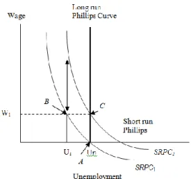
The Monetarists analysis also is based on adaptive expectation or error learning expectations. Inflation expectations in this case are made using past information. Friedman argues that there is a family of Phillips Curves, each associated with a different expected rate of inflation. If people expected inflation to occur then they would anticipate and expect a correspondingly higher wage rise. Figure 7 presents the expectations augmented Phillips curve.
Figure 7. Expectations Augmented Phillips Curve Source: Friedman (1976) and Snowdon & Vane (2005)
Assuming that the economy starts in the equilibrium at point A, in which unemployment is at its natural rate, and wage rate is zero, and then government decides that it wants to lower the level of unemployment because it is too high. If the government reduces unemployment below the natural rate, Un, to U1 by expanding aggregate demand through expansionary monetary policy, then wage will rise to W1. This is because excess demand in goods and labour markets would
result in upward pressure on prices and money wages, with commodity prices adjusting more rapidly than wages (Snowdon & Vane, 2005)
Assuming that the policy measure is not anticipated, this increase in wage will be perceived by workers as an increase in their real wages and supply more labour; that is, they would suffer from temporary money illusion. In this case, the economy will be at point B on the short-run Phillips curve (SRPC1), where unemployment is
reduced and money wages have risen while real wages have fallen. After adjusting their expectations, workers start to seek for additional money wages to compensate the decline in their real wages. They would press for increased money wages, shifting the short-run Phillips curve upwards from SRPC1 to SRPC2.Money wages
would rise at a rate of W1 plus the expected rate of inflation (Friedman, 1976 and Snowdon & Vane, 2005). Since firms cannot pay the high wage rate that workers seek, unemployment returns back to its natural rate and the economy settles at point C (Makuria, 2013). Hence, in the long-run unemployment is at its natural rate but wage is inflated to W1 (Friedman 1976).At the natural rate the labour market is
in a state of equilibrium and the actual and expected rates of inflation are equal; that is, inflation is fully anticipated (Snowdon & Vane, 2005).
If inflation is expected to be higher, the short-run Phillips Curve is also expected to shift to the right (Makuria, 2013). If higher inflation is anticipated then there will be no short-run effect for expansionary monetary policy (Makuria, 2013). However, if the policy measure is not anticipated then there will be a short-run effect (Friedman 1976). Thus, according to Monetarists, there is a positive short-run relationship between inflation and economic growth, provided that the growth is accompanied by the decline of unemployment and rise in the cost of production leading to price inflation. This short-run relationship exists if and only if the policy measure to raise the aggregate demand is not anticipated (Makuria, 2013). In such cases, when workers adjust their expectations output adjusts to its natural rate at the vertical long-run Phillips Curve leaving the price higher. As a result, an increase in money supply will increase the pricelevel without having any
effect on output and hence there will be no long-run trade-off between inflation and economic growth (Friedman, 1976).
3.1.5. The New Keynesians View
New Keynesian economics developed in response to the perceived theoretical crisis within Keynesian economics (Snowdon & Vane, 2005). The paramount task facing Keynesian theorists is to remedy the theoretical flaws and inconsistencies in the old Keynesian model. Therefore, new Keynesian theorists aim to construct a coherent theory of aggregate supply where wage and price rigidities can be rationalized (Snowdon & Vane, 2005). The New Keynesians combine the Keynesian recognition that the economy does not adjust instantly and smoothly to shocks, including monetary shocks, with an insistence on building their explanation on microeconomic foundations (Dornbusch & Fischer, 1990). Wages and prices are assumed to be rigid and thus the level of inflation remains unchanged (Vaona, 2011). These rigidities play an important role in exaggerating economic shocks that arise from either the demand or the supply side (Blanchard & Gali 2005). For example, if money supply is tightened then aggregate demand declines leading to lower economic growth and higher unemployment.
New Keynesians believe that fall in the aggregate demand leads to lower productivity by firms. This also implies that firms will produce only up to the level where they get demand for their production. Since prices are rigid or take a long time to adjust, there will be no market for additional produced commodities even at lower prices (Ball et. al., 1988). Furthermore, the New Keynesians argue that even if prices and wages are flexible, high and unstable prices affect productivity negatively. For example, during a period of recession, risk avoiding firms prefer to reduce their output rather than dealing with the fluctuation of prices and the associated uncertainties (Makuria, 2013).
New Keynesian models state that targeting the optimal inflation rate leads to optimal rate of growth and unemployment. In inflation targeting monetary policies, credibility of the policy is very important and hence the Central Bank’s independence plays a crucial role in this case (Ambler, 2008). Furthermore, New Keynesians argue that to achieve rapid economic growth and to have fair distribution of income there must be low and stable inflation. This implies that high inflation has a negative effect on both economic stability and growth. According to New Keynesians, an attempt to reduce inflation through tightened money supply leads to recession. This is because firms have the ability to set prices, and they may often be reluctant to cut prices leading to price rigidity. Thus, in order to set monetary policy there has to be prior information about future values of inflation and output (Makuria, 2013). For New Keynesians, inflation whether anticipated or unanticipated, has an overall negative impact on economic growth (Ambler, 2008). Inflation creates costs in the economy.
3.1.6 Endogenous Growth Theory
Endogenous growth theory is implicated in the traditional and strengthening microeconomic foundations of neoclassical economics. It describes economic growth which is generated by factors within the production process, for example; economies of scale, increasing returns or induced technological change; as opposed to exogenous factors such as the increases in population (Gokal & Hanif, 2004). In endogenous growth models the long-run growth of income per capita depends on investment decisions rather than unexplained technological progress (Snowdon & Vane, 2005)1. The rate of return on a firm’s accumulation of capital determines
1
The term investment in the context of endogenous growth models refers to a broader concept than the physical capital accumulation reported in the national accounts; research and development
growth rate and that the production function includes technology
A asendogenous input (equation 7).
K L A
FY , , (7)
Economists under endogenous growth theory argue that, at the micro level, the output of an individual firm
i depends on its own inputs of capital Ki ,labour Li and the economy-wide state of knowledge
A (Snowdon & Vane,2005) as presented in model (8).
K L A
F
Yi i, i, (8)
The model implies that technology
A depends on capital stock. At the sametime technology affects capital. Growth is an endogenous process. The higher the capital stock the more the economy is able to use new technologies, which in turn increases productivity of all firms. The growth of technology is assumed to depend on the growth of capital because capital deepening fosters technological spillovers that raise the marginal productivity of capital across the economy as a whole. The expansion of aggregate knowledge or technology, results from learning externalities among firms (Romer, 1986). Snowdon & Vane (2005) ascertain that the higher the level of the capital stock in an economy, the more productive each firm will be via a process of learning by doing. The basic intuition is that although a firm’s production function exhibits constant returns to scale and diminishing returns to capital accumulation, the aggregate production function exhibits increasing, rather than constant, returns to scale (Snowdon & Vane, 2005). The endogenous growth models reveal that the rate of return on human capital and physical capital must be equal in the balanced growth equilibrium. However, a tax on either form of capital induces a lower return. Inflation is expected to reduce growth rate because it leads to fall in rate of return, which in turn reduces capital accumulation.
In fact, Gokal & Hanif (2004) shows that when endogenous growth models are set within a monetary exchange framework, of Lucas (1980), Lucas & Stokey (1987), or McCallum & Goodfriend (1987), the inflation rate (tax) lowers both the return on all capital and the growth rate. They also ascertain that a tax on capital income directly reduces the growth rate, while a tax on human capital would cause labour to leisure substitution that lowers the rate of return on human capital and can also lower the growth rate.
Overall, the relationship between inflation and economic growth as revealed by theoretical literature is mixed. Some contributions produce a negative and significant relationship between inflation and growth (Haslag, 1998; Gillman & Kejak, 2004; Gomme, 1993 and Gillman et al., 1999). Other contributions produce a positive and significant impact of inflation on growth (Tobin, 1965) while other theories produce insignificant long run effect of inflation on growth (Dotsey & Sarte, 2000 and Chari et al., 1996).
3.2. Empirical Literature Review
Studies on the relationship between inflation and economic growth are concerned with not just a simple relationship between the two variables but also whether the relationship holds in the long run or just a short run phenomenon,
(R&D) expenditures and human capital formation may also be included (Crafts, 1996 and Snowdon & Vane, 2005).
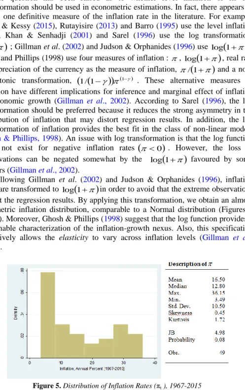
causal direction of the relationship, and whether the relationship is linear or non linear. One of the most important contributions to the inflation-economic growth literature is provided by Khan & Senhadji (2001). Khan & Senhadji (2001) analyze the inflation and growth relationship separately for industrial and developing countries. They use panel data set spanning from 1960 to 1998 for 140 countries. They also re-examine the existence of threshold effects in the relationship between inflation and growth, using econometric techniques initially developed by Chan & Tsay (1998), and Hansen (1999; 2000). However, the main drawback of the paper is the use of an unbalanced panel due to short-span of data mostly in developing countries. To test for the existence of a threshold effect, the log of inflation is preferred. They suggest that regressions of real GDP growth on the level of inflation instead of the log, would give greater weight to the extreme observations, with the potential to skew the results. They propose that the log transformation eliminate, at least partially, the strong asymmetry in the inflation distribution. The paper employs the threshold point Conditional Least Squares (CLS) to estimate the model for each assigned values for the threshold level in the model. The results indicate that threshold levels of inflation that minimize the Residual Sum of Square (RSS) are 1-3 percent for industrialized countries and 7-11 percent for developing countries. These results suggest that inflation levels below the threshold levels of inflation have no effect on growth, while inflation rates above the threshold have a significant negative effect on growth. Generally, Khan & Senhadji (2001)’s results provide a strong evidence for supporting the view of low inflation for sustainable growth. However, the estimated relationship between inflation and growth does not provide the precise channel through which inflation affects growth. Investment and employment are considered in the estimation as control variables.
Similarly, Li (2006) analyzes the nonlinear relationship between inflation and economic growth and the channels through which inflation affects growth in the long run. The paper uses data for 27 developed countries and 90 developing countries spanning from 1961 to 2004. Both simple linear regression and fixed effect estimations are used. The empirical results suggest threshold levels of 14 percent and 38 percent for the developing countries in the sample. Between these levels of inflation the effect of inflation on growth is negative and significant. When the inflation level is below 14 percent, the effect is insignificant but when the level of inflation is above 38 percent the effect diminishes but remains significantly negative. Also, the study finds that total factor productivity is the main channel through which inflation affects growth. Likewise, Ghosh & Phillips (1998) analyze the nonlinearity of the inflation-growth relationship using a data set of 3,603 annual observations for 145 countries, during the 1960-1996 period. The results show that at very low rates of inflation, about 2 to 3 percent per annum, inflation and economic growth are positively correlated. Otherwise, inflation and economic growth are negatively correlated. This implies that the relationship is convex, so that the decline in growth associated with an increase in inflation from 10 percent to 20 percent is much larger than that associated with moving from 40 per cent to 50 percent. They also reveal that inflation is one of the most important statistical determinants of economic growth. Ghosh & Phillips (1998)’s results confirms early study by Fischer (1993). Indeed, Fischer (1993) examines the non-linear relationship between inflation and output growth using both cross-sectional and panel data of 93 countries including developing and industrial countries. As it is revealed in Ghosh & Phillips (1998), Fischer (1993) shows that at low rates of inflation, the relationship between inflation and economic growth is positive but the relationship becomes negative as the inflation rises suggesting a non-linear relationship between the variables. In addition, Fischer (1993) reveals that the strength of the relationship weakens for inflation rates above 40 percent. Mubarik
(2005) also employs the method developed by Khan & Senhadji (2001) to investigate the threshold level of inflation for Pakistan, using annual time series data spanning from 1973 to 2000. The paper includes control variables such as population and investment. Variables used in the model are transformed into log so as to get rid of asymmetry in inflation distribution. The paper employs the Granger Causality test as an application of the threshold model and the relevant sensitivity analysis of the model. The estimation results of the threshold model suggest that an inflation rate above 9 per cent is detrimental for the growth in Pakistan. It also suggests that inflation rate below the critical level of 9 per cent is favourable for growth in the country.
Sarel (1996) also tests for the existence of a threshold effect between inflation and economic growth using a panel data of 87 countries, covering the 1970-1990 period. An OLS regression is estimated for the growth rate on the inflation dummies and other variables such as population growth rate, initial income per person, government expenditure-to-GDP ratio and the rate of change in terms of trade. The test presents evidence that the function that relates economic growth to inflation contains a structural breakpoint of an annual inflation rate of 8 percent. The results imply that below the inflation rate of 8 percent, inflation does not have a significant impact on economic growth, or it may even show a slightly positive effect but above that level, the effect of inflation on growth is negative, significant, robust and very powerful. The existence of a structural break suggests a specific numerical target for policy to keep inflation below the structural break. In a similar paper, Bruno & Easterly (1998) examine the determinants of economic growth using cross-sectional data of 26 countries for the 1961-1992 period. The main argument under their paper is that the negative correlation between inflation and growth exists only in high frequency data and with extreme inflation observations. The robustness of the results is examined by controlling for other factors such as political crises, terms of trade shocks and wars. Their empirical results suggest that the relationship between inflation and growth is negative when a threshold level of inflation is over 40 percent. Below this threshold however, they find inconclusive relationship between the two variables when countries with high inflation crisis are excluded from the sample. They argue that at lower rates of inflation, growth and inflation may simply be jointly troubled by various demand and supply shocks and hence shows no consistent pattern.
Nonexistence of long run relationship between inflation and growth is supported by Moshiri & Sepehri (2004) who like many other authors test the non-linearities in the inflation-growth nexus for industrial and developing countries. Indeed, the empirical results of this paper is that, one, the turning points varies widely from as high as 15 percent for lower middle income countries to 11 percent for low-income countries, and 5 percent for upper-middle-income countries. Second, there is no statistically significant long-run relationship between inflation and growth for OECD countries. However, the results point out the possible bias in the estimation of the inflation and growth nexus that may emanate from combining various countries at different levels of development (Rutayisire, 2013). Nonetheless, Jha & Dand (2011) reveal the same results, that there is no significant effect of inflation variability on economic growth when inflation is high. Here the method used to detect threshold levels in inflation variability is measured by the coefficient of variation. Also, the estimation uses five-year averages to eliminate multicollinearity for panel data consisting of 31 developed countries for the1961-2009 period. Apart from growth rate and inflation, the estimation equation consists of other variables namely terms of trade, initial income level government consumption expenditure gross capital formation over GDP, the growth rate of money and quasi money. Moreover, Faria & Carneiro (2001), applying a bivariate
vector autoregression, find no long-run relationship between inflation and economic growth in Brazil. But in the short run the results suggest the existence of a negative relationship.
The other panel study that estimates threshold level of inflation is undertaken by Kremer et al. (2009). Indeed, Kremer et al. (2009) expand the scope of Khan & Senhadji (2001) by modelling a large panel-data set of 124 industrialized and non-industrialized countries over the 1950-2004 period. A dynamic panel threshold model is employed in the analysis for the growth equation. The empirical results suggest that the inflation threshold level is about 2.5 percent for industrial countries and 17 percent for non-industrialized economies. The paper also reveals that below the threshold of 2.5 percent, the effect of inflation on long-term growth is significantly positive in developed countries but the impact of inflation on growth remains insignificant in developing economies when inflation is below 17 percent. In fact, the paper fails to support the growth-enhancing effects of inflation on growth in developing economies.
Barro (1995) explores the inflation-growth nexus using a panel data for 100 countries over the 1960-1990 period. He estimates growth regression using Instrumental Variables (IV) technique. The empirical results suggest that there exists a statistically significant negative relationship between the inflation and economic growth, with a coefficient of -0.024. The results also suggest that if a number of the country characteristics are held constant, then the effects from an increase in average inflation by 10 percentage points per year are a reduction of the growth rate of real per capita GDP by 0.2-0.3 percentage points per year, and a decrease in the ratio of investment to GDP by 0.4-0.6 percentage points. Motely (1998), in a cross-country study with a data set covering the same period, also reveals a similar relationship. He suggests that an increase in inflation of 5 percent leads to a 0.1 to 0.5 percent decrease of economic growth.
Recent studies also imply different conclusions on the optimal level of inflation that would maximize growth (Yabu & Kessy, 2015; Rutayisire, 2013; Seleteng et al., 2010; Paul, 2012; Hayat, 2013 and Younus, 2012). Moreover, most of the studies on the nonlinear effect of inflation on economic growth use cross-sectional or panel data covering a large number of countries. Understandably, many of previous studies confirm the existence of nonlinear relationship between inflation and economic growth in the different country specific cases albeit with different levels of threshold. The lack of consensus regarding the optimal threshold level is evident. Insufficiency of techniques stems, in part, from exogenous determination of the threshold levels, failure to control for unobserved heterogeneity at both country and time levels, or failure to account for cross sectional dependence (Bittencourt, et al., 2014). These important discrepancies in the findings call forth a further investigation with recent data and methods, to explore the extent to which inflation affects economic growth. In this perspective, it is important to investigate the inflation-growth nexus in developing countries like Tanzania covering a large sample, spanning from 1967 to 2015. The empirical results of this paper are expected to contribute to the ongoing debate on the inflation-growth relationship.
4. Data
This paper uses annual time series data of Tanzania, for the 1967-2015 period. Inflation rate and the growth rate of real GDP at 2005 prices are obtained from the World Development Indicators (2016). The control variables include the investment as the share of GDP, the rate of population growth, the degree of openness or trade (measured as exports plus imports as the share of GDP) and