Washington University in St. Louis
Washington University in St. Louis
Washington University Open Scholarship
Washington University Open Scholarship
Mechanical Engineering and Materials Science
Independent Study
Mechanical Engineering & Materials Science
12-19-2016
Uncertainty Quantification (UQ) for Wall Modeled Large Eddy
Uncertainty Quantification (UQ) for Wall Modeled Large Eddy
Simulation (WMLES) Model
Simulation (WMLES) Model
Zuoxian Hou
Washington University in St. Louis
Ramesh K. Agarwal
Washington University in St. Louis
Follow this and additional works at: https://openscholarship.wustl.edu/mems500
Recommended Citation
Recommended Citation
Hou, Zuoxian and Agarwal, Ramesh K., "Uncertainty Quantification (UQ) for Wall Modeled Large Eddy Simulation (WMLES) Model" (2016). Mechanical Engineering and Materials Science Independent Study. 20.
https://openscholarship.wustl.edu/mems500/20
This Final Report is brought to you for free and open access by the Mechanical Engineering & Materials Science at Washington University Open Scholarship. It has been accepted for inclusion in Mechanical Engineering and Materials Science Independent Study by an authorized administrator of Washington University Open Scholarship. For more information, please contact [email protected].
E37-MEMS500-09: Independent Study Report – Fall 2016
Uncertainty Quantification (UQ) for
Wall Modeled Large Eddy Simulation (WMLES) Model
Zuoxian Hou and Ramesh K. AgarwalWashington University in St. Louis, St. Louis, MO, 63130
In this paper non-intrusive uncertainty quantification (UQ) method is used to improve the accuracy of Smagorinsky Large eddy simulation (LES) model and a wall-modeled large eddy simulation (WMLES) model. Detailed UQ studies focusing on the closure coefficients of these two models are performed. A Polynomial Chaos (PC) surrogate model is used to evaluate the output sensitivities and uncertainties in the entire flow domain. The proposed UQ method allows for the investigation of specific flow features and phenomena within the domain. The results of the UQ analyses are then used to identify which closure coefficients in the models most influence the flow features of interest. Refinements are then made to the closure coefficients of interest to improve the accuracy of the two LES models. OpenFOAM is used as the flow solver and the UQ analyses are conducted with DAKOTA. The proposed UQ method is applied to the turbulent channel flow at various Reynolds numbers. The LES models with new closure coefficients show significant improvement in the prediction of the skin-friction coefficient on channel walls.
I.
Introduction
Interest in uncertainty quantification (UQ) in computational fluid dynamics (CFD) has grown in recent years. UQ has been successfully applied to design, optimization, and modeling problems, and is becoming a standard tool for verification and validation of numerical solutions. The development of non-intrusive UQ methods has reduced the computational expense of UQ and has allowed uncertainty propagation through complex models without alteration to the underlying model.
In the present work the sensitivities of the closure coefficients of the Smagorinsky model, and the wall-modeled large eddy simulation (WMLES) model were investigated. Flow calculations were performed with OpenFOAM. Channel Flow with different Reynolds number is considered.
Non-intrusive polynomial chaos is used to propagate the uncertainty in the closure coefficients. DAKOTA is used to calculate the Sobol indices which quantify the sensitivity of each coefficient to some physical quantity of interest. The quantities of interest are the coefficients of skin friction. Details of the turbulence models, flow solvers, and test cases are given in the next sections. Results and discussions of the UQ analyses are presented. Closure coefficients of interest are identified.
II.
LES Models
A. Smagorinsky Model
In order to close the equations and thereby determine the filtered velocity field u(x, t) and the modified filtered pressure
p
(x, t), we need to model the anisotropic residual-stress tensorτ
ij (x, t). The Smagorinsky model is the simplest model and has been proven to perform reasonably well.In this model, the anisotropic residual-stress tensor
τ
ijis related to the filtered rate-of-strain)
(
2
1
)
(
:
)
(
ij j i i j ij ijS
u
S
u
u
u
S
=
=
=
∂
+
∂
as ij t t ijν
S
τ
=
−
2
This is the mathematical realization of the Boussinesq hypothesis, that turbulent fluctuations are dissipative in the mean. The mathematical structure is similar to that of molecular diffusion. The filtered momentum equation can be written as
,
)
)
((
2
i t ij j j j i i j iu
+
u
∂
u
=
∂
+
S
−
∂
p
+
f
∂
ν
ν
j
=
1
,
2
,
3
.
The residual subgrid-scale eddy viscosity νr acts as an artificial viscosity and represents the eddy viscosity of the residual motions. It is modeled as 2 1 2 2 1 2
)
2
(
)
(
)
2
(
lk lk s lk lk s t=
S
S
=
C
∆
S
S
ν
Here, we have the Smagorinsky lengthscale
s= Cs∆, the Smagorinsky coefficient Cs and the filter width ∆. Finally, we can write the filtered momentum equation as,
)
)
)
2
(
((
2
2 1 2 j j ij lk lk s i j t i j tu
+
u
∂
u
=
∂
+
S
S
S
−
∂
p
+
f
∂
ν
j
=
1
,
2
,
3
.
In OpenFoam the Smagorinsky coefficient Cs is calculated by two coefficients which are named Ck and Ce. The relationship between Cs and Ck, Ce can be written as:
ε
C
C
C
C
k k s=
The model constants and their recommended bounds are shown in Table 1. These bounds were determined based on the behavior of the model when applied to canonical free shear flows and a turbulent channel flow boundary layer.
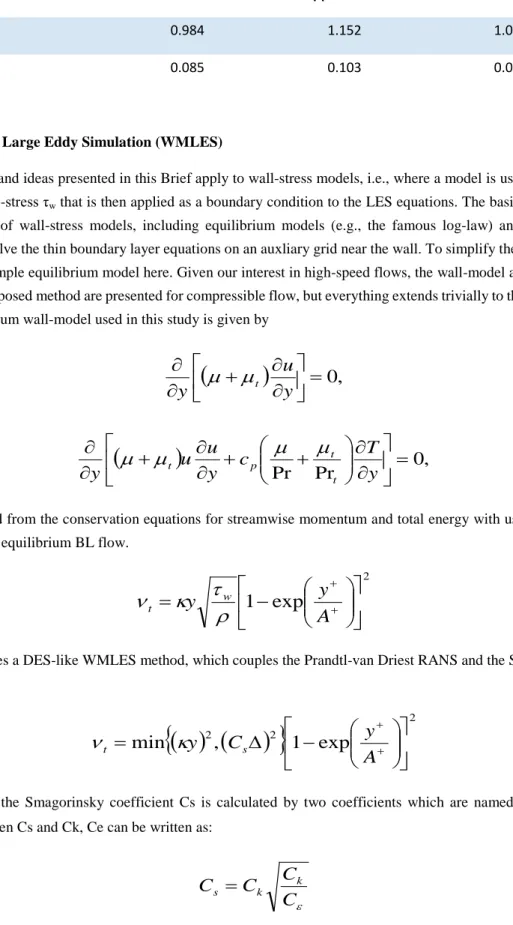
Table 1Epistemic Intervals of Closure Coefficients for Smaorinsky model.
Closure Coefficient Lower Bound Upper Bound Standard Value
Ck 0.984 1.152 1.048
Ce 0.085 0.103 0.094
B. Wall-Modeled Large Eddy Simulation (WMLES)
The arguments and ideas presented in this Brief apply to wall-stress models, i.e., where a model is used to estimate the instantaneous wall-stress τw that is then applied as a boundary condition to the LES equations. The basic reasoning holds for a wide range of wall-stress models, including equilibrium models (e.g., the famous log-law) and more elaborate approaches that solve the thin boundary layer equations on an auxliary grid near the wall. To simplify the presentation, we consider only a simple equilibrium model here. Given our interest in high-speed flows, the wall-model and the arguments leading to the pro-posed method are presented for compressible flow, but everything extends trivially to the incompressible case. The equilibrium wall-model used in this study is given by
(
)
=
0
,
∂
∂
+
∂
∂
y
u
y
µ
µ
t(
)
0
,
Pr
Pr
=
∂
∂
+
+
∂
∂
+
∂
∂
y
T
c
y
u
u
y
t t p tµ
µ
µ
µ
which was derived from the conservation equations for streamwise momentum and total energy with use of the standard approximations in equilibrium BL flow.
2
exp
1
−
=
++A
y
y
w tρ
τ
κ
ν
The simulation uses a DES-like WMLES method, which couples the Prandtl-van Driest RANS and the Smagorinsky SGS models:
( ) (
)
{
}
2 2 2exp
1
,
min
−
∆
=
++A
y
C
y
s tκ
ν
In OpenFoam the Smagorinsky coefficient Cs is calculated by two coefficients which are named Ck and Ce. The relationship between Cs and Ck, Ce can be written as:
ε
C
C
C
C
k k s=
The model constants and their recommended bounds are shown in Table 2. These bounds were determined based on the behavior of the model when applied to canonical free shear flows and a turbulent channel flow boundary layer.
Table 2Epistemic Intervals of Closure Coefficients for WMLES model.
Closure Coefficient Lower Bound Upper Bound Standard Value
Ck 0.984 1.152 1.048
Ce 0.085 0.103 0.094
κ 0.37 0.45 0.41
III.
Flow Solver Verification
OpenFOAM is an open source CFD software package written in C++. It has continued to gain popularity and grow its user base in part thanks to the ease of modification of its code. It has an impressive range of mesh tools, solvers, and pre-post processing tools. Before using it in the present study, the current implementations of the Smagorinsky and WMLES models were verified for the channel flow case of the turbulence fileserver of texas.
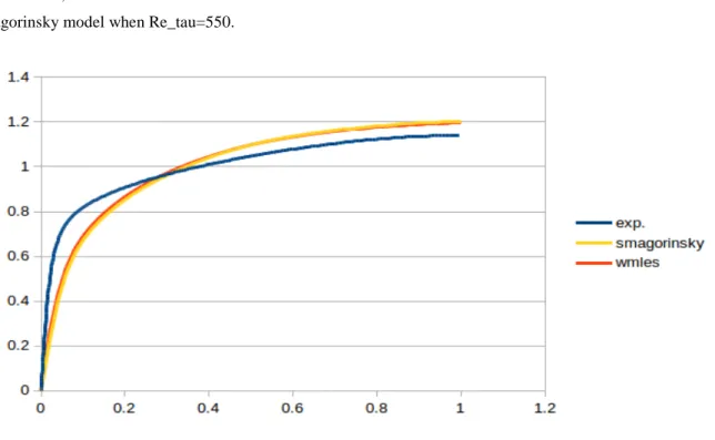
When Re_tau=550, the velocity profile of Smagorinsky model, WMLES model and experimental data is shown like Figure 1. It can be seen that the the maximum value of velocity from experimental data is 1.14m/s, from Smagorinsky model is 1.203m/s, from WMLES model is 1.196m/s. It can be referred that result from WMLES model is more accurate than Smagorinsky model when Re_tau=550.
Fig. 1 Velocity profile at Re_tau-550
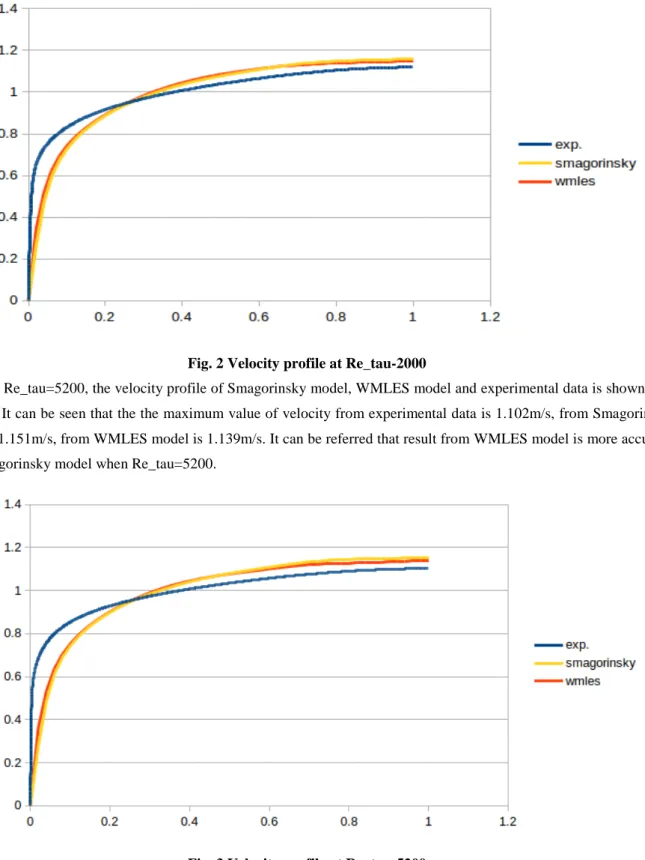
When Re_tau=2000, the velocity profile of Smagorinsky model, WMLES model and experimental data is shown like Figure 2. It can be seen that the the maximum value of velocity from experimental data is 1.119 m/s, from Smagorinsky model is 1.158m/s, from WMLES model is 1.149m/s. It can be referred that result from WMLES model is more accurate than Smagorinsky model when Re_tau=2000.
Fig. 2 Velocity profile at Re_tau-2000
When Re_tau=5200, the velocity profile of Smagorinsky model, WMLES model and experimental data is shown like Figure 3. It can be seen that the the maximum value of velocity from experimental data is 1.102m/s, from Smagorinsky model is 1.151m/s, from WMLES model is 1.139m/s. It can be referred that result from WMLES model is more accurate than Smagorinsky model when Re_tau=5200.
Fig. 3 Velocity profile at Re_tau-5200
Above all, it can be inferred that whatever the Reynolds number is, the result of WMLES model is always more accurate than it in the Smagorinsky model. The reason of that may come from the inner layer, WMLES model did a better job than Smagorinsky model in the part which is near the wall.
IV.
Test Cases
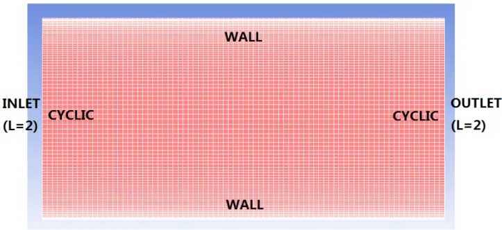
A turbulent channel flow is a widely used simple verification and validation test case. The Reynolds number of the flow is Re_tau= 550, 2000, and 5200. The computational grids used were taken from the tutorial of channel flow with Re_tau=395. The computational grid with every other node and boundary conditions are shown in Figures 5 respectively. This case is used to determine the typical sensitivities of the model coefficients so that comparisons to more complex cases can be made.
Fig. 4 Mesh and BC for the channel flow
V.
Results
The following tables describe the sensitivity of the named turbulence model to changes in the models’ closure coefficients for the channel flow with different Reynolds number case. OpenFOAM was used as the flow solver as stated above Sobol Indices, computed by SANDIA National Labs DAKOTA software, were used to rank the influence of each coefficient.
Tables 3 and 4 show the sensitivity analysis results obtained from OpenFOAM for the skin friction coefficients with Re_tau=2000 and Re_tau=5200.
Comparing the sensitivities between different Reynolds number with same turbulent model, it can be seen that when turbulence model is Smagorinsky model, Sobol Indices of Ck don’t have a big variety, but Sobol Indices of Ce goes down along with decreasing Reynolds number.When turbulence model is chosen as WMLES model, it can be seen that similar with Smagorinsky model, Sobol Indices of Ck seems no change. However, Sobol Indices of Ce decreases with decresing Reynolds number, and in contact, Sobol Indices of κ increases with decreasing Reynolds number.
Comparing the sensitivities between different turbulent models with same Reynolds number, it can be seen when changing turbulence model from Smagorinsky to WMLES, Sobol Indices of Ck decreases and Sobol Indices of Ce increases.
Comparing the sensitivities in one certain model, it can be seen that in the Samgorinsky model,the Ck, is a more significant contributor to the uncertainty than Ce. The most significant coefficient for the WMLES model for the skin friction coefficient is changing with variety of Reynolds number. The coefficient that makes the least influence in WMLES model is Ck.
Table 3 Sobol Indices for the skin friction coefficient from OpenFOAM at Re_tau=2000
Smagorinsky WMLES
Coefficient Sobol Indices Coefficient Sobol Indices
Ck 0.2826 Ck 0.0779
Ce 0.1105 Ce 0.5394
κ 0.1032
Table 4 Sobol Indices for the skin friction coefficient from OpenFOAM at Re_tau=5200
Smagorinsky WMLES
Coefficient Sobol Indices Coefficient Sobol Indices
Ck 0.272 Ck 0.0889
Ce 0.0178 Ce 0.2797
κ 0.4651
VI.
Conclusions
In this paper an uncertainty quantification methodology has been successfully implemented in OpenFOAM. UQ studies focusing on the closure coefficients of eddy-viscosity turbulence models for several flows were performed. Three eddy viscosity turbulence models were considered: the Smagorinsky model, and the Wall-modeled Large Eddy Simulation model. Sobol Indices were used to rank the contributions of each constant to total model uncertainty. This study is intended as motivation and information for those who desire to advance turbulence models towards more accurate formulations.
For the case of a turbulent channel flow, it was found that the Smagorinsky model exhibited particular sensitivity to Ck, Ce contributes a very less part when Reynolds number continues to increase. When tested in OpenFOAM, the WMLES model showed less than 5% to total uncertainty to Ck when the skin friction coefficient was considered the quantity of interest, while Ce and κ affected by the different Reynolds number.
VII.
Future Work
In the future, the next step is to make research on when Reynolds number continues to change (increase or decrease), what will happen on the variety of Sobol Indices of every coefficient in Smagorinsky model and WMLES model. After that, Sobol Indices on other coefficient by Ck, Ce and κ can also be an interesting point to further. Last but not least, UQ of these two models on other cases attracts me,too. It will be done in my next plan.
References
1
Mikhail L.Shur, Philippe R. Spalart, Mikhail Kh.Strelets and Andrey K.Travin, “A hybrid RANS-LES approach with delayed-DES and wall-modelled LES capabilities,” International Journal of Heat and Fluid Flow 29 (2008) 1638-1649; 2Macro Rosler, “the Smagorinsky turbulence model,” [D], Institute of Mathematics of Freie University Berlin, 2015 3Brendan D. Tracey, “Machine Learning for Model Uncertainties in Turbulence Models and Monte Carol Integral Arreoxiamation,” [D], Stanford University, June 2015
4J. Larsson and S. Kawai, “Wall-modeling in large eddy simulation: large scales, grid resolution and accuracy,” Center for Turbulence Research Annual Research Briefs, 2010