Discovering Data Quality Rules

(1)

Discovering Data Quality Rules

∗

Fei Chiang

University of Toronto

Ren ´ee J. Miller

University of Toronto

ABSTRACT

Dirty data is a serious problem for businesses leading to incorrect decision making, inefficient daily operations, and ultimately wasting both time and money. Dirty data often arises when domain constraints and business rules, meant to preserve data consistency and accuracy, are enforced in-completely or not at all in application code.

In this work, we propose a new data-driven tool that can be used within an organization’s data quality management process to suggest possible rules, and to identify confor-mant and non-conforconfor-mant records. Data quality rules are known to be contextual, so we focus on the discovery of context-dependent rules. Specifically, we search for condi-tional funccondi-tional dependencies (CFDs), that is, funccondi-tional dependencies that hold only over a portion of the data. The output of our tool is a set of functional dependencies to-gether with the context in which they hold (for example, a rule that states for CS graduate courses, the course number and term functionally determines the room and instructor). Since the input to our tool will likely be a dirty database, we also search for CFDs that almost hold. We return these rules together with the non-conformant records (as these are potentially dirty records).

We present effective algorithms for discovering CFDs and dirty values in a data instance. Our discovery algorithm searches for minimal CFDs among the data values and prunes redundant candidates. No universal objective measures of data quality or data quality rules are known. Hence, to avoid returning an unnecessarily large number of CFDs and only those that are most interesting, we evaluate a set of interest metrics and present comparative results using real datasets. We also present an experimental study showing the scalability of our techniques.

1. INTRODUCTION

Poor data quality continues to be a mainstream issue for many organizations. Having erroneous, duplicate or incom-∗_{Supported in part by NSERC and NSF 0438866.}

Permission to copy without fee all or part of this material is granted provided that the copies are not made or distributed for direct commercial advantage, the VLDB copyright notice and the title of the publication and its date appear, and notice is given that copying is by permission of the Very Large Data Base Endowment. To copy otherwise, or to republish, to post on servers or to redistribute to lists, requires a fee and/or special permission from the publisher, ACM.

VLDB ‘08,August 24-30, 2008, Auckland, New Zealand

plete data leads to ineffective marketing, operational inef-ficiencies, inferior customer relationship management, and poor business decisions. It is estimated that dirty data costs US businesses over $600 billion a year [11]. There is an in-creased need for effective methods to improve data quality and to restore consistency.

Dirty data often arises due to changes in use and per-ception of the data, and violations of integrity constraints (or lack of such constraints). Integrity constraints, meant to preserve data consistency and accuracy, are defined ac-cording to domain specific business rules. These rules define relationships among a restricted set of attribute values that are expected to be true under a given context. For example, an organization may have rules such as: (1) all new cus-tomers will receive a 15% discount on their first purchase and preferred customers receive a 25% discount on all pur-chases; and (2) for US customer addresses, the street, city and state functionally determines the zipcode. Deriving a complete set of integrity constraints that accurately reflects an organization’s policies and domain semantics is a primary task towards improving data quality.

To address this task, many organizations employ consul-tants to develop a data quality management process. This process involves looking at the current data instance and identifying existing integrity constraints, dirty records, and developing new constraints. These new constraints are nor-mally developed in consultation with users who have specific knowledge of business policies that must be enforced. This effort can take a considerable amount of time. Furthermore, there may exist domain specific rules in the data that users are not aware of, but that can be useful towards enforcing semantic data consistency. When such rules are not explic-itly enforced, the data may become inconsistent.

Identifying inconsistent values is a fundamental step in the data cleaning process. Records may contain inconsis-tent values that are clearly erroneous or may poinconsis-tentially be dirty. Values that are clearly incorrect are normally easy to identify (e.g., a ’husband’ who is a ’female’). Data values that are potentially incorrect are not as easy to disambiguate (e.g., a ’child’ whose yearly ’salary’ is ’$100K’). The unlikely co-occurrence of these values causes them to become dirty candidates. Further semantic and domain knowledge may be required to determine the correct values.

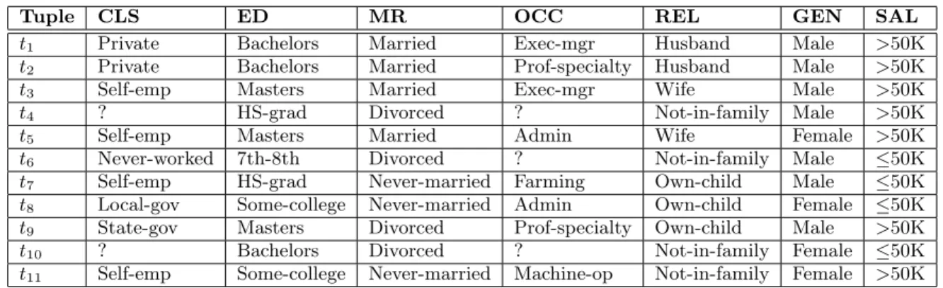
For example, Table 1 shows a sample of records from a 1994 US Adult Census database [4] that contains records of citizens and their workclass (CLS), education level (ED), marital status (MR), occupation (OCC), family relationship (REL), gender (GEN), and whether their salary (SAL) is

(2)

Table 1: Records from US 1994 Adult Census database

Tuple CLS ED MR OCC REL GEN SAL

t1 Private Bachelors Married Exec-mgr Husband Male >50K

t2 Private Bachelors Married Prof-specialty Husband Male >50K

t3 Self-emp Masters Married Exec-mgr Wife Male >50K

t4 ? HS-grad Divorced ? Not-in-family Male >50K

t5 Self-emp Masters Married Admin Wife Female >50K

t6 Never-worked 7th-8th Divorced ? Not-in-family Male ≤50K

t7 Self-emp HS-grad Never-married Farming Own-child Male ≤50K

t8 Local-gov Some-college Never-married Admin Own-child Female ≤50K

t9 State-gov Masters Divorced Prof-specialty Own-child Male >50K

t10 ? Bachelors Divorced ? Not-in-family Female ≤50K

t11 Self-emp Some-college Never-married Machine-op Not-in-family Female >50K

above or below $50K. We intuitively recognize the following inconsistencies:

1. Int3, if the person is a married male, then REL should

beHusbandnotW if e. Alternatively, the GEN should beF emale. This is clearly an erroneous value. 2. The tuplet6indicates a person with a missing

occupa-tion (where the ”?” indicates a NULL) and a workclass indicating he has never worked. Support in the data reveals that when occupation is missing so is the work-class value, indicating that if the person is temporarily unemployed or their occupation is unknown, so is their workclass. Given this evidence, the discrepancy in t6

indicates either the value ”Never-worked” is dirty and should be ”?”; or a semantic rule exists to distinguish people who have never been employed and their salary must be less than $50K (versus those who are tem-porarily unemployed or their occupation is unknown). 3. The tuple t9 represents a child (under 18) who is

di-vorced with a salary over $50K. Most children are un-married and do not have such a high salary.

Cases (2) and (3) are potential exceptions whereby an analyst with domain knowledge can help to resolve these inconsistencies, and may enforce new rules based on these discrepancies.

In this paper, we propose a new data-driven tool that can be used during the data quality management process to suggest possible rules that hold over the data and to identify dirty and inconsistent data values. Our approach simplifies and accelerates the cleaning process, facilitating an interactive process with a consultant who can validate the suggested rules (including rules that may not be obvi-ous to users) against business requirements so that they are enforced in the data, and with a data analyst who can re-solve potential inconsistencies and clean the obvious dirty values. As described above, data quality rules are known to be contextual, so we focus on the discovery of context-dependent rules. In particular, we search for conditional

functional dependencies (CFDs) [5], which are functional

dependencies that hold on a subset of the relation (under a specific context). For example, the earlier business rules can be expressed as CFDs:

• φ1a:[status = ’NEW’, numPurchases = 1]→ [discount = 15%]

• φ1b:[status = ’PREF’]→[discount = 25%]

• φ2:[CTRY = ’US’, STR, CTY, ST]→[ZIP]

Similarly, the semantic quality rules for the Census data can be represented as:

• φ3:[MR = ’Married’, GEN = ’Male’]→ [REL = ’Husband’]

• φ4:[CLS = ’Never-worked’]→[OCC = ’?’, SAL = ’≤ $50K’]

• φ5:[REL = ’Own-child’]→[MR = ’Never-married’, SAL = ’≤ $50K’]

In this paper we formalize and provide solutions for dis-covering CFDs and for identifying dirty data records. In particular, we make the following contributions:

• We present an algorithm that effectively discovers CFDs that hold over a given relationR. We prune redundant candidates as early as possible to reduce the search space and return a set of minimal CFDs.

• We formalize the definition of an exception (dirty) value and present an algorithm for finding exceptions that violate a candidate CFD. Exceptions are iden-tified efficiently during the discovery process. Once found, they can be reported back to an analyst for verification and correction.

• To avoid returning an unnecessarily large number of CFDs and only ones that are most interesting, we eval-uate a set of interest metrics for discovering CFDs and identifying exceptions. Our results show that convic-tion is an effective measure for identifying intuitive and interesting contextual rules and dirty data values. • We present an experimental evaluation of our

tech-niques demonstrating their usefulness for identifying meaningful rules. We perform a comparative study against two other algorithms showing the relevancy of our rules, and evaluate the scalability of our techniques for larger data sizes.

The rest of the paper is organized as follows. In Section 2, we present related work and in Section 3 we give preliminary definitions and details of our rule discovery algorithm. In

(3)

Section 4, we present our algorithm for identifying records that are exceptions to approximate rules and lead to dirty data values. Section 5 presents an experimental evaluation of our methods and Section 6 concludes our paper.

2. RELATED WORK

Our work finds similarities to three main lines of work: functional dependency discovery, conditional functional de-pendencies, and association rule mining.

Functional dependency (FD) discovery involves mining for all dependencies that hold over a relation. This includes discovery of functional [13, 18, 24], multi-valued [22] and approximate [13, 16] functional dependencies. In previous FD discovery algorithms, both Tane [13] and DepMiner [18] search the attribute lattice in a levelwise manner for a mini-mal FD cover. FastFDs [24] uses a greedy, heuristic, depth-first search that may lead to non-minimal FDs, requiring fur-ther checks for minimality. We generalize the lattice based levelwise search strategy for discovering CFDs.

Conditional functional dependencies, are a form of con-strained functional dependencies (introduced by Maher [19]). Both Maher and Bohannon et al. [5] extend Armstrong’s ax-ioms to present a (minimal) set of inference rules for CFDs. To facilitate data cleaning, Bohannon et al. [5] provide SQL based techniques for detecting tuples that violate a given set of CFDs. Both of these papers have assumed that the CFDs are known, which is not always true. Manual discovery of CFDs is a tedious process that involves searching the large space of attribute values. None of the previous work has focused on this problem.

Recent work in conditional dependencies has focused on conditional inclusion dependencies (CIND) and finding re-pairs for tuples violating a given set of CFDs. Inclusion dependencies are extended with conditional data values to specify that the inclusion dependencies hold over a subset of the relation. Bravo et al. [6] study the implication and consistency problems associated with CINDs and their in-teraction with CFDs, providing complexity results, infer-ence rules and a heuristic consistency-check algorithm. Con-straint based data cleaning searches for a repair database

D0 _{that is consistent with the CFDs and differs minimally} from the original databaseD. Cong et al.[9] propose repair algorithms to repairDbased on the CFDs and potential up-dates toD. We focus on discovering CFDs and identifying tuples that violate these rules. Any of the proposed repair algorithms can be used to clean the reported dirty tuples.

There are many statistical approaches for error localiza-tion, again, assuming the data quality rules are known (and valid) where the goal is to find errors or rule violations [23]. Many data cleaning tools support the discovery of statis-tical trends and potential join paths [10], schema restruc-turing and object identification [21, 12], but to the best of our knowledge none of these tools focus on the discovery of contextual dependency rules.

Association rule mining (ARM) focuses on identifying re-lationships among a set of items in a database. The se-mantics of association rules differ from CFDs. In ARM, for itemsetsU, V, the ruleU →V indicatesU occurs withV. However,U may also occur with other elements. CFDs de-fine a strict semantics where for a set of attributesX, Y, a CFDX → Y indicates that the values in X must (only) occur with the corresponding values in Y. Large itemsets that satisfy minimum support and confidence thresholds are

Table 2: CFD φ: ([STAT, NUM-PUR] →[DISC],T1)

STAT NUM-PUR DISC

’New’ 1 15

’Pref’ ’−’ 25

most interesting [1, 2]. Statistical significance and convic-tion tests [7] have also been used to assess itemset quality. We employ some of these measures to evaluate the quality of a CFD during our discovery process.

One of the foundational techniques in ARM, the Apriori algorithm [3], builds large itemsets by adding items only to large itemsets and pruning small itemsets early that do not satisfy the support threshold. A superset of a small itemset will remain small, hence the itemset can be pruned to reduce the number of itemsets considered. This is known as theanti-monotonic property. In our work, applying this pruning technique to our classes of data values may lead us to miss groupings of smaller constant values that together may form a valid condition satisfying the support threshold. We eliminate conditioning on attributes whose maximum class size is less than the support level since their supersets will also fall below the support level.

Related to ARM, frequent pattern mining searches for frequent itemsets that satisfy domain, class, or aggregate constraints [14, 15, 20, 17]. This helps to focus the min-ing on desired patterns. A primary objective is to discover data patterns involving similar values defined by (given) domain widths [14, 15]. Similar to the anti-monotonic prop-erty, optimizations for computing frequent patterns involve constraint push down [20], and pruning strategies that are specific to the constraint type [17]. Both ARM and frequent pattern mining focus on value based associations, whereas our techniques focus on finding rules that allow variables not just constant values.

3. SEARCHING FOR DATA QUALITY RULES

Given a relation R, we are interested in finding all data quality rules that exist inRand that satisfy some minimum threshold. As data quality rules are contextual, we search for conditional functional dependencies (CFD), which are functional dependencies that hold under certain conditions. We first give some preliminary definitions.

3.1 Preliminaries

A CFDφoverR can be represented byφ: (X →Y, Tp)

[5], where X, Y are attribute sets in R and X → Y is a functional dependency (FD). Tp is a pattern tableau of φ,

containing all attributes in X and Y. For each attribute

B in (X ∪Y), the value of B for a tuple in Tp, tp[B], is

either a value from the domain of B or ’−’, representing a variable value. For example, the rules φ1a and φ1b are

represented as rows in Table 2. A CFD enhances functional dependencies by allowing constant values to be associated with the attributes in the dependency. In particular, CFDs are able to capture semantic relationships among the data values.

A tuple t matches a tuple tp in tableau Tp if for each

attribute B in Tp, for some constant ’b’, t[B] = tp[B] =

’b’ or tp[B] = ’−’. For example, the tuple (’Pref’,10,25)

(4)

a relationR satisfies the CFDφ, denoted asI |=φ, if for every pair of tuplest1andt2inI, and for each pattern tuple

tp inTp, ift1[B] = t2[B] for every attribute B inX, and

botht1, t2 match tp[B], then t1[A] = t2[A] andt1, t2 both

matchtp[A] for attribute A inY. Tuplet inR violatesφ

ift[B] =tp[B] = ’b’ ortp[B] = ’−’ for every attributeB in

X, but t[A]6=tp[A] for attribute AinY. Without loss of

generality, we consider CFDs of the formϕ: (X →A, tp),

whereAis a single attribute andtpis a single pattern tuple.

The general formφ: (X→Y, Tp) can be represented in this

simpler form as (X →A, tp(X∪A)) for eachAinY andtpin

Tp. Intuitively, we decomposeY into its singular attributes

and consider each resulting dependency individually. This is equivalent to applying the decomposition rule1 _{[5, 19].}

CFDs of this form areminimal (in standard form) whenA

does not functionally depend on any proper subset ofX so that each attribute inX is necessary for the dependency to hold. This structural definition also holds for FDs.

We search for CFDs whereX may contain multiple vari-ablesP and (X−P) conditional attributes. For X →A, if the consequentA resolves to a constant ’a’ for all values in variable(s)P (tp[P] = ’−’), then we report ’a’ in tpand

removeP from the rule since it has no effect on the value of A. Returning a constant value rather than a variable

A, along with the conditional values, enables the rules to provide increased information content.

In the next section, we describe the attribute partition model and how quality rules are generated. We then present the metrics that we use to evaluate the quality of a discov-ered rule, followed by a discussion of the pruning strategies we adopt to narrow the search space and to avoid redundant candidates.

3.2 Generating Candidates

Letnbe the number of attributes inRand letXbe an at-tribute set ofR. ApartitionofX, ΠX, is a set of equivalence

classes where each class contains all tuples that share the same value inX. Letxirepresent an equivalence class with

a representativeithat is equal to the smallest tuple id in the class. Let|xi|be the size of the class andvibe the distinct

value ofX that the class represents. For example, in Table 1 forX1=MR, ΠMR={{1,2,3,5},{4,6,9,10},{7,8,11}}, for

X2=REL, ΠREL ={{1,2},{3,5},{4,6,10,11},{7,8,9}}, and

forX3= (MR,REL), Π(MR, REL)={{1,2},{3,5},{4,6,10},{9},

{11},{7,8}}. For ΠM R,x7 ={7,8,11},|x7|= 3, andv7 = ’Never-married’. A partition ΠXrefinesΠY, if everyxiin

ΠXis a subset of someyiin ΠY [13]. The FD test is based on

partition refinement where a candidate FDX →Y overR

holds iff ΠXrefines ΠY. Since CFDs hold for only a portion

of R, the CFD test does not require complete refinement, that is, it does not require every class in ΠX to be a subset

of some class in ΠY. We will elaborate on this shortly.

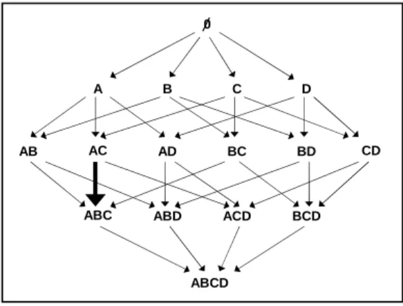
To find all minimal CFDs, we search through the space of non-trivial2_{and non-redundant candidates, where each}

can-didate is of the formγ:X →Y, and test whetherγ holds under a specific condition. A candidateγ is non-redundant if its attribute sets X, Y are not supersets of already dis-covered CFDs. The set of possible antecedent values is the collection of all attribute sets, which can be modeled as a set containment lattice, as shown in Figure 1. Each node in the lattice represents an attribute set and an edge exists

1_{Decomposition rule: If}_X _→_{Y Z}_{, then}_X_→_Y _and_X_→_Z 2_{A candidate}_X_→_A_{is trivial if}_A_⊆_X_.

0

A B C D

AC AD BC BD CD

AB

ABC ABD ACD BCD

ABCD

Figure 1: Attribute search lattice

between setsXandY ifX⊂Y andY has exactly one more attribute than X, i.e.,Y =X∪ {A}. We define a candidate CFD based on an edge (X, Y) as follows.

Definition 1. An edge (X, Y) in the lattice generates a

candidate CFD γ : ([Q, P]→A) consisting of variable

at-tributes P andQ = (X −P) conditional attributes, where

Y = (X∪A). P andQconsist of attribute sets that range

over the parent nodes ofX in the lattice.

For example, in Figure 1, for edge (X, Y) = (AC, ABC), we consider conditional rules γ1: ([Q=A,C]→B) andγ2:

([Q=C,A]→B), whereQranges over the parent nodes of

AC, and will take on values from these attribute sets. For the single attribute case, (X, Y) = (A, AB), we consider the conditional rule γ: ([Q = A, ∅] → B). For the rest of the paper, we will use this notation (based on attribute sets) to represent candidate CFDs.

Each candidateγis evaluated by traversing the lattice in a breadth-first search (BFS) manner. We first consider all

X consisting of single attribute sets (at level k = 1), fol-lowed by all 2-attribute sets, and we continue level by level to multi-attribute sets until (potentially) level k =n−1. We only visit nodes on the BFS stack that represent mini-mal CFD candidates. The algorithm efficiency is based on reducing the amount of work in each level by using results from previous levels. In particular, by pruning nodes that are supersets of already discovered rules and nodes that do not satisfy given thresholds, we can reduce the search space (by avoiding the evaluation of descendant nodes) thereby saving considerable computation time.

CFD validity test For attribute sets X, Y a class xi in

ΠX is subsumed by yi in ΠY if xi is a subset of yi. Let

ΩX ⊆ΠX represent all the subsumed classes in ΠX. Let

X = (P∪Q) whereP represents variable attributes andQ

the conditional attributes, then γ: ([Q, P]→A) is a CFD iff there exists a class qi in ΠQ that contains values only

from ΩX.

Intuitively, the CFD validity test is based on identifying values inXthat map to the sameY value. Since values are modeled as equivalence classes, we are interested inxi that

do not split into two or more classes inY (due to attribute A). If there is a conditionQthat the tuples in ΩX share in

(5)

is generally preferable to find rules that hold for more than one, or indeed for many, tuples. Hence, we may additionally impose a constraint that|xi|> lfor some threshold valuel.

Example 1. The search for CFDs in Table 1 begins at

level k = 1 and we setl = 1. Consider the following

par-titions (for brevity, we show only a subset of the attribute partitions): • ΠMR={{1,2,3,5},{4,6,9,10},{7,8,11}} • ΠREL={{1,2},{3,5},{4,6,10,11},{7,8,9}} • Π(R,M)3={{1,2},{3,5},{4,6,10},{7,8},{9},{11}} • ΠED={{1,2,10},{3,5,9},{4,7},{6},{8,11}} • ΠCLS={{1,2},{3,5,7,11},{4,10},{6},{8},{9}} • Π(C,E)={{1,2},{10},{3,5},{4},{6},{7},{8},{9},{11}} • Π(M,E)={{1,2},{10},{3,5},{9},{4},{6},{7},{8,11}} • Π(M,E,C)={{1,2},{10},{3,5},{9},{4},{6},{7},{8},{11}}

For edge (X, Y) =(REL, (REL, MR)),x1 andx3 are the

subsumed classes. SinceX is a single attribute, if we take

Q=X=RELandP =∅, then we can conditionQonv1, v3,

to obtain the rulesϕ1: ([REL = ’Husband’]→MR) andϕ2:

([REL = ’Wife’] → MR) as CFDs. Since the values in x1

andx3 each map to the constant ’Married’, we return the

more informative rule ϕ1 : ([REL = ’Husband’] → [MR =

’Married’]) (similarly for ϕ2), indicating that if a person

is a husband, then he must be married.

Consider the edge(X, Y) = (ED, (ED, CLS)), there are

no subsumedxiclasses. After evaluating edges from level-1,

we consider edges from level-2 nodes. Now consider the edge

(X, Y)=((ED,MR), (ED,MR,CLS)). The classesx1 andx3

are subsumed and contained in Ω(ED,MR). We check if there

exists a classqiinΠQ=MR that contains only values fromx1 andx3. We see thatq1={1,2,3,5}satisfies this requirement.

Therefore, by the CFD test we returnϕ: ([MR = ’Married’,

ED]→[CLS]) as a conditional data quality rule.

The traversal continues to nodes representing CFD can-didates that require further evaluation. We use informa-tion about discovered CFDs from previous levels to prune the search space and avoid evaluating redundant candidates. We will elaborate on this pruning strategy in Section 3.5.

3.3 Multiple Variables and Conditional

At-tributes

The CFDϕis true if there exists some valueq(condition onQ) that holds over ΩX. The remaining non-subsumed

classes ΛX= (ΠX−ΩX) are not considered during the

con-ditioning. If there is no conditional valueqthat is true over ΩX, then there does not exist a dependency with

condition-ing attributesQ. However, the classes in ΩX can still be

refined by considering additional variable and conditional attributes. In particular, we consider the updated set of at-tributesX0_{(with added variables and conditions), and test} whether a rule exists over the classes in ΩX0.

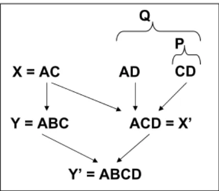
First, we consider adding another variable attribute B. Considering an extra attribute can help to further restrict

3_{For brevity, we abbreviate}_(REL,MR)_to_(R,M)

X = AC AD Y = ABC ACD = X’ Y’ = ABCD CD Q P

Figure 2: A portion of the attribute search lattice classes that previously were not subsumed. When a can-didateγ:X →Acorresponding to an edge (X, Y) fails to materialize to a CFD, we generate a new candidateX0_→_Y0 in the next level of the lattice where X0 _{= (}_X_∪_B_{) and}

Y0_{= (}_Y _∪_B_),_B₆₌_A_{. The variable attributes}_P _{range over} the attribute sets that are parents ofX0 _{and (}_X0₋_P_{) is the} current conditional attribute. See Figure 2 for an example. If γ: ([A,C] → B) with conditional nodeA, corresponding to edge (X, Y) = (AC, ABC) does not materialize to a CFD, a new candidate based on the edge (X0_{, Y}0_{) will be} evalu-ated. Specifically,γ0_{: (}_[A,C,D]_→_B_{) will be considered with} variable attributesC,D.

If a candidate rule does not materialize to a CFD after adding a variable attribute, then we condition on an addi-tional attribute. Similar to adding variables, we consider conditional attributes Qthat range over the attribute sets that are parents of X0 _{(see Figure 2). We add these new} candidates (X0_{, Y}0_{) to a global candidate list} _G_{and mark} the corresponding lattice edge (X0_{, Y}0_{). We perform the} CFD test only for classes in ΩX0. At level k ≥ 2, where multi-condition and multi-variable candidates are first con-sidered, we only visit nodes with marked edges to ensure minimal rules are returned, and thereby also reducing the search space.

Example 2. Continuing from Example 1, the evaluation

of edge (X, Y) = ((REL), (REL, MR)) produced classes x4

and x7 that were not subsumed. Consider edge(X0, Y0) =

(SAL,REL), (SAL, REL, MR)), withγ: [Q=(SAL),REL]→

[MR]. The attribute partitions are:

• ΠSAL={{1,2,3,4,5,9,11},{6,7,8,10}}

• Π(SAL,REL)={{1,2},{3,5},{4,11},{9},{6,10},{7,8}}

• Π(S,R,M)={{1,2},{3,5},{4},{11},{9},{6,10},{7,8}}

Classesx1, x3, x6, x7 are subsumed classes. However, we

do not condition using x1 and x3 since a CFD was found

previously with these classes. We consider only x6 and x7

inΩ(X=SAL,REL). UnderQ=(SAL), we check for aqiinΠQ

that contains only tuple values from ΩX. The class q1 fails

since it contains tuple values not inΩX, butq6={6,7,8,10}

with v6 =’≤50K’ qualifies. All tuple values inx6 and x7

share the same conditional valuev6, hence,[SAL = ’≤50K’,

REL]→[MR]is a conditional data quality rule.

After visiting all marked edges, the set of discovered rules and their conditional contexts are reported to the user. Al-gorithm 1 presents pseudocode to identify conditional data quality rules overR.

(6)

Algorithm 1Algorithm to discover CFDs INPUTRelationR, current levelk

1: InitializeCL={},G={} 2: foreachX in levelkdo 3: consider (marked) edge (X, Y) 4: if |ΠX|=|ΠY|then

5: {(X, Y) represents an FD}. Unmark edge (X, Y), remove its supersets fromG.

6: else 7: ΩX= subsumedxi, ΛX= (ΠX−ΩX) 8: findCFD(ΩX, X, Y, k) 9: if ΩX6=∅then 10: G(X0_{, Y}0_{, Q, P}_{) = (Λ} X,ΩX) {Generate next

CFD candidate; add variable, conditional at-tributes. Mark edge (X0_{, Y}0_)._}

11: if k≥2 andG=∅then

12: break{No candidates remaining} 13: return CL{List of conditional rules}

DEFINE findCFD(ΩX, X, Y, k)

1: Ifk≥2: itn = 2, ELSE itn = 1 2: fori: 1 to itndo

3: {First check for CFDs with added variables. If none found, check with added conditions.}

4: forqi in ΠQdo

5: if qi contains values only from ΩX then

6: if M(xi, yi)≥τ then

7: ϕ: X →A{M: interest metric,τ: threshold} 8: CL= (CL∪ϕ){add discovered CFD to list} 9: ΩX = (ΩX - (xiinϕ)){update classes}

10: If CFDs found, break. 11: return (ΩX)

3.4 Interest Measures for CFDs

To capture interesting rules we consider three interest measures, namely support, theχ2_{-test, and conviction. We}

apply these metrics as a filter to avoid returning an unnec-essarily large number of rules, and to prune rules that are not statistically significant nor meaningful.

3.4.1 Support

Support is a frequency measure based on the idea that values which co-occur together frequently have more evi-dence to substantiate that they are correlated and hence are more interesting. The support of a CFDϕ: (X →A),

support(X→A), is the proportion of tuples that matchϕ, defined as

Sϕ=s=# tuples containing values inX andA

N=# of tuples inR (1)

For an attribute setX,support(X) is defined as the num-ber of tuples containing values in X divided by N. If ϕ

holds, then s = Σ|yi|, for yi that subsumexi in ΩX. For

example, the ruleϕ:[SAL = ’≤50K’, REL]→[MR]holds forx6, x7 in Ω(SAL,REL), which are subsumed by y6, y7 in

Y. Hence,s=|y6|+|y7|= 2 + 2 = 4, givingSϕ = (4/11).

In our algorithm, we only consider rules that exceed a mini-mum support thresholdθ, that is, we are interested in rules withSϕ≥θ.

3.4.2

χ2

_-Test

Givenϕ:X →A, we expect the support of ϕto be the frequency in which the antecedent and consequent values occur together, i.e., (support(X)∗support(A)). If the actual support support(X → A) deviates significantly from this expected value, then the independence assumption between

X and A is not satisfied. Rules withsupport(X → A) ≈ (support(X)∗support(A)) are not interesting. We capture this idea by using theχ2 _test

χ2=(E(vXvA)−O(vXvA)) 2 E(vXvA) + (E( ¯vXvA)−O( ¯vXvA))2 E( ¯vXvA) + (E(vXv¯A)−O(vXv¯A))2 E(vXv¯A) + (E( ¯vXv¯A)−O( ¯vXv¯A))2 E( ¯vXv¯A) (2)

Let vX, vA be the set of constant values in ϕ from X

andA, respectively. O(vXvA) represents the number of

tu-ples containing bothvX and vA (including conditional

val-ues). E(vXvA) is the expected number of tuples

contain-ing vX and vA under independence, that is, E(vXvA) = O(vX)O(vA)

N , whereO(vX) is the number of tuples wherevX

occurs. Similarly,O( ¯vX) is the number of tuples wherevX

does not occur. Theχ2 _{value follows a}_χ2 _{distribution. We}

test for statistical significance by comparing theχ2_{value to}

critical values from standard χ2 _{distribution tables. For a}

critical value of 3.84, only in 5% of the cases are the variables independent ifχ2 _{is greater than 3.84. Hence, if}_χ2 _>₃_.₈₄

then the valuesX →AunderQare correlated at the 95% confidence level. We apply theχ2_{test both on its own and}

in conjunction with support to filter rules that are not sta-tistically significant according to a given significance level.

3.4.3 Conviction

Various measures have been proposed to quantify mean-ingful attribute relationships and to capture interesting rules. Confidence is one of these measures. The confidence of ϕ: (X→A) can be stated as

Confidence=Cfϕ=P r(X, A)

P r(X) =

P r(Q, P, A)

P r(Q, P) (3) whereX= (Q∪P) andP r(Q, P) is equal tosupport(Q, P). Confidence measures the likelihood that Aoccurs given P

under condition Q. We can compute this value by taking the number of occurrences ofP andA(withQ) and divid-ing this by the number of occurrences ofP (withQ). IfP

always occurs withAthen the confidence value is 1. If they are independent, then confidence is 0. A drawback of confi-dence is that it does not consider the consequentA, and it is possible that P r_{P r}(Q,P,A₍_Q,P₎) =P r(Q, A), indicating thatP and

A are independent. If this value is large enough to satisfy the desired confidence threshold, then an uninteresting rule is generated.

Interest is an alternative correlation metric that measures how much two variables deviate from independence. The interest ofϕquantifies the deviation ofP andA(with con-ditionQ) from independence. We define interest forϕas

Interest=Iϕ= P r(Q, P, A)

P r(Q, P)P r(Q, A) (4) The valueIϕ ranges from [0,∞]. IfIϕ>1 this indicates

(7)

that knowingPincreases the probability thatAoccurs (un-der conditionQ) . IfP andAare independent thenIϕ= 1.

AlthoughIϕ considers both P r(Q, P) andP r(Q, A) it is a

symmetric measure, that fails to capture the direction of the implication inϕ.

The asymmetric conviction metric [7] addresses this short-coming. It is similar to interest but considers the directional relationship between the attributes. The conviction forϕis defined as

Conviction=Cϕ=P r(Q, P)P r(¬A)

P r(Q, P,¬A) (5)

ϕ: ((Q, P)→A) can logically be expressed as¬((Q, P)∧ ¬A), and conviction measures how much ((Q, P)∧ ¬A) deviates from independence. WhenP and Aare independent, con-viction is equal to 1, and when they are related concon-viction has a maximal value approaching∞. We apply these inter-est measures in our CFD validity tinter-est as shown in Algorithm 1. A qualitative study evaluating these measures is given in Section 5.2.

3.5 Pruning

We apply pruning rules to efficiently identify a set of min-imal, non-redundant CFDs inR.

Conditioning Attributes. If a candidate X → A is a functional dependency overR, then all edges (XB, Y B) representing supersets of edge (X, Y) are pruned. This is because (X∪B) →Acan be inferred fromX →A. Fur-thermore, supersets ofXA→C for all other attributes C

inR are also pruned, since we can remove A without af-fecting the validity of the dependency (whether it holds or not) and hence, is not minimal. For CFDs, we must take extra care since for each distinct conditional attribute value

Qinϕ:X→A, we get different tuple values satisfying the rule (sinceϕ holds only over a portion of the relation). If

ϕholds under conditionQ, we prunexi in ΩX from being

considered in subsequent evaluations of ϕ with conditions that are supersets ofQ. This is to ensure that the discov-ered rules are minimal. For example, ifQ =U, then xi ²

ΩX are not considered in subsequent evaluations involving

Q = U V, U V W, etc.They are however considered in rules with conditions not includingU. We maintain a hash table that records whichxito consider for a candidate rule under

specific conditional attributes. The set ΛX is updated to

remove subsumedxi as rules are discovered. For example,

in Example 1 we will consider only x4 and x7 for

candi-dates involving supersets of (X, Y) = ((REL), (REL,MR))

with conditions that are supersets of (REL).

Support Pruning. In support, we leverage the

anti-monotonic property [3] that if support(X) < θ, then any

supersets ofX will also fall belowθ. If a setX is not large enough, then adding further attributes results in a new set that is either equal to or smaller thanX. The first intuition is to apply this property to prune|xi|< θ. For example,

sup-pose for candidate (X, Y) =((SAL,REL), (SAL,REL,MR))in Example 2,θ = 0.3. All the classesx1, x3, x6 and x7 have

size equal to 2 and fall belowθ, and hence should be pruned. However, if we were interested in only finding value based rules, this would work. But we are interested in finding rules that also contain variables. The ruleϕ: [SAL = ’≤50K’, REL] → [MR] holds under condition SAL = ’≤50K’ (class

x0

6 ={6,7,8,10}in ΠSAL) having support(X →A) = 4≥θ.

We do not prune classes inXwhose individual sizes are less thanθsince the sum of these class sizes may satisfyθunder a common conditional value. Instead, we prune based on |qi|inQ. If the largest class inQis less thanθ, then clearly

the current candidate rule does not contain sufficient sup-port. Furthermore, any supersets of Qwill also fall below

θ. We maintain a list of these small conditional attribute sets and prune all candidate rules with conditions involving these small sets.

Frequency Statistics. When evaluating an edge (X, Y) in the first level of the lattice (where X and Y resolve to single value constants), we can leverage attribute value fre-quency statistics to prune CFD candidates in the reverse direction. Suppose we are considering a candidateϕ: [X = ’Toronto’]→[Y = 416]. If the partition classes|xT oronto|=

|y416|thenϕis a CFD. The value |y416|represents the

co-occurrence frequency between the values ’416’ and ’Toronto’. The actual frequency count of value ’416’, f416, may be

larger than|y416|, indicating that ’416’ co-occurs with other

X values. This indicates that the reverse CFD candidate [Y

= 416]→[X = ’Toronto’] does not hold. More specifically, for a CFD [X = ’x’]→ [Y = ’a’], whereX is a single at-tribute, Y = (X∪A), if (fa ≤ya) for some value ’a’ in A,

then the reverse CFD [A= ’a’]→[X = ’x’] holds. Other-wise, they-class representative should be saved for further conditioning on multiple attributes. Note that we do not need to explicitly store thefavalues since these are the class

partition sizes for the single attributeA. This process allows us to evaluate two CFD candidates (A →B, B →A) for the price of one, and we are able to prune half of the level-1 candidates, saving considerable computational effort.

4. IDENTIFYING DIRTY DATA VALUES

Real data often contains inconsistent and erroneous val-ues. Identifying these values is a fundamental step in the data cleaning process. A data value can be considered dirty if it violates an explicit statement of its correct value. Al-ternatively, if no such statement exists, a value can be con-sidered dirty if it does not conform to the majority of values in its domain. In particular, if there is sufficient evidence in the data indicating correlations among attribute values, then any data values participating in similar relationships, but containing different values are potentially dirty. We for-malize this intuition and search for approximate CFDs over

R. If such approximate rules exist, then there are records that do not conform to the rules and contain potentially dirty data values. We report these non-conformant values along with the rules that they violate. We define what it means for a value to be dirty using the support and convic-tion measures.

4.1 Using Support

A conditional rule ϕ : X → A is true if there is some condition q that holds for xi in ΩX. The remaining

non-subsumed classes xi in ΛX, are not considered during the

conditioning. Each of theseximaps to two or more classes

yk in ΠY indicating that theX value occurs with different

Y values. Let ΥY be the set ofyk ²ΠY thatxi²ΛX maps

to. Letymax represent the largestyk class, and recall that

θis the minimum support level. If|ymax| ≥(θ∗N) and∃ys

such that|ys| ≤ (α∗N), ys 6= ymax, then ψ = ([X = vi]

→[Y =vs]) is reported as a violation. The parameterαis

(8)

(percentage) of a dirty data value. Similar thresholds have been used to find approximate FDs, where the threshold defines the maximum number of violating tuples allowed in order for an FD to qualify as approximate [13].

Intuitively, since there is no 1-1 mapping between any of thexi in ΛX and a specificyk in ΥY, a CFD cannot hold

over these values. However, we can check if there is aymax

that satisfiesθ, and if so, then this is an approximate CFD (i.e., if the remainingykclasses did not exist then ([X=vi]

→ [Y = vmax] would be a CFD). We select ymax to be

the largest class. The remaining vk values co-occur with

vi at different frequencies, and if there are vk values that

occurinfrequently (less thanα), then they are inconsistent with respect to vmax. Once a set of dirty data values is

found for a candidate (X, Y), the corresponding classes xi

are not considered again (for dirty values) in rules involving supersets of (X, Y). This is to avoid returning redundant dirty values from the same record.

Example 3. Returning to our Census Table 1, let θ =

0.15 and α = 0.1. We remarked that tuples t3, t6 and t9

contained dirty values and we show how these values can be identified. Consider the following attribute partitions:

• Π(M,G)={{1,2,3},{5},{4,6,9},{10},{7},{8,11}}

• Π(M,G,R)={{1,2},{4,6},{3},{5},{7},{8},{9},{10},{11}}

• ΠOCC={{1,3},{2,9},{4,6,10},{5,8},{7},{11}}

• ΠCLS={{1,2},{3,5,7,11},{4,10},{6},{8},{9}}

• Π(C,O)={{1},{2},{3},{5},{4,10},{6},{7},{8},{9},{11}}

Consider candidate (X, Y) = ((MR, GEN), (MR, GEN, REL))

and class x1 = (1,2,3), which maps to y1 = (1,2) and

y3 = (3). Since ymax = y1 and |y_N1| ≥ θ, and ys = y3,

|y3|

N ≤α, we have a dirty value in tuple t3. That is,[MR =

’Married’, GEN = ’Male]→[REL = ’Wife’]is

inconsis-tent with the rule[MR = ’Married’, GEN = ’Male]→[REL

= ’Husband’].

For candidate (X, Y) = ((OCC), (OCC, CLS)),x4= (4,6,10)

maps toy4 = (4,10)andy6= (6). Similar to above,ymax=

y4, ys = y6, and we have a non-conformant tuple t6 with

dirty values[OCC = ’?’]→[CLS = ’Never-worked’]

vio-lating[OCC = ’?’] →[CLS = ’?’] with support = (2/11).

Similarly, we discover the following inconsistent values int9:

[REL = ’Own-child’] → [MR = ’Divorced’] and [REL =

’Own-child’]→[SAL = ’>50K’] which violate ϕ1:[REL

= ’Own-child’]→[MR = ’Never-married’]and ϕ2:[REL

= ’Own-child’]→[SAL = ’≤50K’], respectively.

Dirty data values can prevent underlying rules from be-ing discovered and bebe-ing reported concisely. A larger set of CFDs are generated to get around the exception. For exam-ple, if a record contains [’Husband’]→[’Female’], the ac-tual CFD [’Husband’]→[’Male’] does not hold, and an in-creased number of rules such as [’Husband’, ’Doctorate’] →[’Male’] and [’Husband’, ’Exec-mgr’] →[’Male’] are found. Our data quality tool is able to identify exceptions along with the potential (and violated) CFD and present these to an analyst for cleaning.

4.2 Using Conviction

We use the conviction measure to identify data values that are independent and violate an approximate CFD. Similar to the support case, we test if an approximate CFD ϕ : ([X = vi] → [Y = vmax]) satisfies a minimum conviction

level C. We sort |yk| in ΥY in descending order to find

rules containing the largest conviction value first. Letymax

represent the satisfyingyk with the largest conviction value

(Cϕ). To identify dirty records, we are interested in finding

all tuples that have independent attribute values relative to ϕ. This means that for theyk, if their conviction value

Cσ < Cϕ, for σ: ([X = vi] → [Y = vk]), then vk has

less dependence with vi than vmax, and hence is reported

as an exception. We rank these exceptions according to descending (Cϕ−Cσ) to find those values that deviate most

fromϕ. Algorithm 2 presents pseudocode for the algorithm to identify dirty data values inR.

Algorithm 2Algorithm to discover dirty data values INPUTRelationR

1: InitializeDL={}dirty list 2: multiSize(xi) = allyi⊆xi

3: foreachxiinmultiSizedo

4: Xbench= 0

5: foryi inmultiSize(xi)do

6: ymax =yiwith largest measureM(xi, yi)

7: if (M(xi, ymax)< τ) and (Xbench== 0)then

8: break{unsatisfied threshold, consider nextxi}

9: else

10: if (Xbench== 0)then

11: Xbench= 1{approximate CFD}

12: ϕ: [X = value ofxi]→[Y = value ofymax]

13: else

14: if M(xi, yi)≤αthen

15: {α: dirty threshold,δ: dirty data value} 16: δ: [X = value ofxi]→[Y = value ofyi]

17: DL= (DL∪(δ, ϕ)){saveδand violated rule

ϕ} 18: returnDL

5. EXPERIMENTAL EVALUATION

We ran experiments to determine the effectiveness of our proposed techniques. We report our results using seven datasets (six real and one synthetic) and provide examples demonstrating the quality of our discovered rules and ex-ceptions.

Real Datasets. We use six real datasets from the UCI Machine Learning Repository [4], namely the Adult, Census-Income (KDD), Auto, Mushroom, Statlog German Credit, and Insurance Company Benchmark datasets. The Adult dataset from the 1994/95 US Census contains 32561 records of US citizens describing attributes related to their salary (above or below $50K). The Census-Income dataset is a larger dataset (similar to Adult) containing 300K tuples (299285 from the original dataset plus we append extra records) with 347 domain values. The Auto dataset de-scribes characteristics of automobiles used for insurance risk prediction, with 205 tuples and 10 attributes. The Mush-room dataset describes physical characteristics of mushMush-rooms and classifies them as either edible or poisonous and contains

(9)

Table 3: Experimental Parameters Parameter Description Values

n number of attributes inR [8,17]

N number of tuples inR [25K, 300K]

d attribute domain size [270, 2070]

θ minimum support level [0.05, 0.5]

8124 tuples with 10 attributes. The Statlog German Credit dataset contains credit information for 1000 customers and rates them with either good/bad credit. Lastly, the Insur-ance Company Benchmark contains 9822 records describ-ing product usage and socio-demographic information on customers from a real insurance company. We use these datasets in our qualitative study described in Section 5.2.

Synthetic Tax Dataset. This is a synthetic dataset consisting of individual US tax records. The data is popu-lated using real data describing geographic zip codes, area codes, states, and cities, all representing real semantic re-lationships among these attributes. Furthermore, real tax rates, tax exemptions (based on marital status, number of children), and corresponding salary brackets for each state are used to populate the tax records. We use this dataset to test the scalability of our techniques.

Parameters. Our experiments were run using a Dual Core AMD Opteron Processor 270 (2GHz) with 6GB of memory. The parameters we evaluate are shown in Table 3. We use theχ2 _{critical value equal to 3.84, representing a}

95% confidence level. We set the minimum conviction level

C = 10 to ensure that a sufficient number of rules are re-turned. We explored different values of θ and αand their individual effect on the discovery time. We observed exper-imentally (using the Adult dataset) that varyingθ (andα) had a minimal effect on the running time. We tested this for eachn= [5,9] and the running times did not vary sig-nificantly. For the qualitative study in Section 5.2, we set confidenceCf = 0.5, and interestI = 2.0 to capture rules that include dependent attributes.

5.1 Scalability Experiments

We used the Tax dataset and varied the parameter of in-terest to test its effect on the discovery running time.

Scalability in N. We studied the scalability of the dis-covery algorithm (with and without identifying exceptions) with respect toN. We considered the support,χ2_{-test, and}

conviction measures. We fixed n = 8, θ = 0.5, α = 0.01 andd = 173. We ran the discovery algorithm forN rang-ing from 25K to 200K tuples. Figure 3 shows the results. The algorithm scales linearly for all the metrics considered. Support and conviction showed the best results (with sup-port marginally outperforming conviction). There is a small overhead for computing exceptions. The results with theχ2

-test did not prune as many rules as expected (forN = 25K, over 234 rules were returned). Furthermore, the rules with the highestχ2_{value were often ones that occurred least}

fre-quently. This lead us to consider support and the χ2_-test

together as a measure to capture rules that are both sta-tistically significant and that have a minimum frequency to substantiate their usefulness. Using the support with the

χ2_{-test returned the same number of rules as using support}

alone, but the χ2_{-test ranks the set of rules satisfying} _θ_.

Since the number of rules returned is equal to the support

0 3 6 9 12 15 18 21 24 27 30 25 50 75 100 125 150 175 200 N - Number of tuples (x1000) ti m e ( m in ) support w/ exceptions support-and-chi-sq support chi-sq conviction conviction w/ exceptions

Figure 3: Scalability in N (Tax dataset)

0 20 40 60 80 100 120 140 50 100 150 200 250 300 N - Number of tuples (x 1000) ti m e ( m in ) support support w/ exceptions conviction conviction w/ exceptions

Figure 4: Scalability inN (Census-Income dataset) measure, we only consider the support measure in subse-quent tests. Figure 4 shows the running times using the real Census-Income dataset with a linear scale-up wrtN up to 300K tuples forn= 8. In both the Tax and Census-Income datasets, the support based measure performs slightly better than conviction particularly for largerN.

Scalability in n. We studied the impact of n on the discovery times. We consideredN = 30K, θ= 0.5, α= 0.01 and d in [12,31]. Figure 5 shows that the number of at-tributes does affect the running time. This is due to the increased number of possible attribute setsX that need to be evaluated. An increased number of attributes causes a larger number of conditions and variables to be evaluated for a candidate rule. For smallern < 15, we observe that the overhead of computing exceptions remains small for both the support and conviction measures. For larger n, this overhead increases more rapidly as there are more poten-tial dirty values to evaluate. For each potenpoten-tial exception, we verify that it has not been considered previously (mini-mal) and that it satisfies theαthreshold. For wide relations (n >15), vertical partitioning of the relation into smaller tables can help reduce the time for finding exception tuples. However, for relations with up ton= 16 attributes, the dis-covery times for rules and dirty values are found reasonably in about 13 and 30 min respectively.

Scalability ind. We evaluate the effect of the domain sizedon the discovery time. We fixN = 30K, n= 6, θ= 0.5 andα= 0.01 and varieddfrom 270 to 2070. Figure 6 shows the results using support and conviction. We expect d to affect the discovery times since an increase in d leads to a larger number of equivalence classes that must be com-pared. The running times using the support measure with and without exceptions are similar, and show a gradual in-crease. The execution times using conviction are slower, and there is an average overhead of about 40% for finding exceptions. This is likely due to weaker pruning strategies for conviction. In support, we prune all supersets of

(10)

condi-0 10 20 30 40 50 60 70 80 90 8 9 10 11 12 13 14 15 16 17 ti m e ( m in ) n - number of attributes support support w/ exceptions conviction conviction w/ exceptions Figure 5: Scalability in n 0 10 20 30 40 50 60 70 80 90 270 470 670 870 1070 1270 1470 1670 1870 2070 d - Domain Size ti m e ( m in ) support support w/ exceptions conviction conviction w/ exceptions Figure 6: Scalability in d

tional attributes that do not satisfy the minimum support level (this property unfortunately does not hold when using conviction). This pruning can have a considerable benefit for increasingdas the number of classes increases. One so-lution to this problem is to group (stratify) the values (when

dis excessively large) to reduce the domain size, where the stratification may be dataset dependent.

5.2 Qualitative Evaluation

We evaluate the quality of the discovered conditional rules and exceptions using the real datasets. Specifically, we con-sider the top-k discovered rules using support, the χ2_-test,

support withχ2_{-test, conviction, confidence and interest.}

Data cleaning is subjective and we do not have a gold standard containing acompleteset of cleaning rules. Hence, we do not report the recall of our approach. However, we can evaluate the rules that are returned based on their use-fulness. Precision is a measure used in information retrieval to measure the percentage of documents retrieved that are relevant to a user’s query. For each top-k set of returned rules, we compute precision to evaluate the effectiveness of each measure in returning rules that are interesting and that are useful towards data cleaning. We do this by manually evaluating each of the top-k rules and selecting those that are most relevant and that convey interesting information.4

We compute the precision for the top-k rules for k = 20. This is also known as theprecision atk, defined as

Precision= # relevant rules

# returned rules (6)

In cases where less thankrules are returned, we setkto the number of returned rules. Table 4 shows the precision for each metric and dataset, along with the total number of rules

4_{This follows a similar process of computing relevance and}

precision in information retrieval where a user study deter-mines the relevance of returned documents for a query.

Table 5: Sample of discovered rules. (*) indicates the rule was also found using conviction.

Support

[OCC = ’?’] →[IND = ’?’] (*)

Unknown occupation implies industry is also unknown [ED = ’Children’]→[SAL = ’≤50K’] (*)

School aged children should make less than $50K [[BODY = ’hatchback’, CYL]→[PRICE]

For hatchbacks, num cylinders determines price [[CLR = ’yellow’, BRUISE, ATTACH]→[CLS] (*)

Yellow mushrooms, bruising and gills imply if it’s poisonous [[PUR = ’education’]→[FGN = ’yes’]

Education loans normally taken by foreign workers Conviction

[RATE = 3]→[DRS = 2] Dangerous cars have two doors [BAL = ’delay’]→[FGN = ’yes’]

Foreign workers normally delay paying off credit [BAL = ’<0’, PUR = ’educ’, AMT]→[RATE] For low, educ loans, amount determines credit rating [S-TYPE = ’large,low class’]→[M-TYPE = ’adult fam’] Lower class families have more adults living together Confidence

([SM=foul,fishy, CLR=’buff’]→[CLS=’poison’] (*) Buff colour mushrooms, foul or fishy smell, are poisonous Interest

([MR = ’single’, PROP = ’yes’]→[LIFE = ’minimal’] Single persons owning property have minimal life insurance

χ2

([S-TYPE = ’76-88% family’]→[LIFE = ’none’] 76-88% of average families have no life insurance ([ED = ’Masters’, FAM]→[SAL]

For Masters educated, family type determines salary range

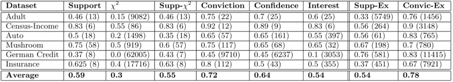
returned in parentheses. Conviction is the superior measure providing the most interesting rules (across all datasets) fol-lowed by confidence, and with support and interest perform-ing similarly. Conviction addresses the limitations of confi-dence, and interest and support, respectively, by considering the consequent and the direction of the implication. Both these characteristics are important for identifying meaning-ful semantic relationships. The German Credit dataset re-turned rules containing specific credit amounts that were not meaningful, hence giving lower precision values.

We found that the χ2_{-test produced an unmanageably}

large number of rules, and rules with high χ2 _values

oc-curred infrequently and were not interesting. This made it difficult to decipher which rules were most important, and manually evaluating each rule was not feasible. Instead, we used theχ2_{-test (with support) to find rules that are}

statis-tically significant after satisfying a minimum support level. This returned a more reasonable number of rules with pre-cision results similar to support. A sample of the discovered rules are given in Table 5. The results show that our tech-nique is able to capture a broad range of interesting rules that can be used to enforce semantic data consistency. This is particularly useful when rules are unknown or are out-dated, and new rules are required to reflect current policies. Many of the rules in Table 5 reveal intuitive knowledge and

(11)

Table 4: Precision results for discovered rules and exceptions. The total total number of returned rules and exceptions are shown in parentheses.

Dataset Support χ2 _Supp-_χ2 _Conviction _Confidence _Interest _Supp-Ex _Convic-Ex

Adult 0.46 (13) 0.15 (9082) 0.46 (13) 0.75 (22) 0.7 (25) 0.6 (25) 0.33 (5749) 0.76 (1456) Census-Income 0.83 (6) 0.55 (86) 0.83 (6) 0.92 (12) 0.89 (9) 0.83 (6) 0.56 (264) 0.9 (3148) Auto 0.5 (18) 0.2 (1498) 0.35 (18) 0.65 (57) 0.65 (161) 0.55 (397) 0.56 (61) 0.83 (765) Mushroom 0.75 (58) 0.5 (919) 0.6 (57) 0.75 (117) 0.65 (68) 0.65 (32) 0.67 (198) 0.7 (780) German Credit 0.37 (8) 0.0 (62005) 0.43 (7) 0.45 (9710) 0.45 (6237) 0.1 (3053) 0.76 (581) 0.83 (11415) Insurance 0.625 (8) 0.4 (17716) 0.63 (8) 0.8 (112) 0.5 (43) 0.5 (355) 0.37 (451) 0.67 (7921) Average 0.59 0.3 0.55 0.72 0.64 0.54 0.54 0.78

Table 6: Sample of dirty values and violated rules. Support

[REL = ’Husband’]→[GEN = ’Female’] Violates: →GEN = ’Male’(*)

[SH = ’Convex’, SM = ’none’]→[CLS = ’edible’] Violates: →CLS = ’poison’(*)

[REL = ’Own-child’]→[SAL = ’>50K’] Violates: →[SAL = ’≤50K’] (*)

Conviction

[MR=’single-male’, PROP=’rent’]→[RATE=’good’] Violates: →RATE = ’bad’

[EMP=’<1yr’, PROP=?] →[RATE=’good’] Violates: →RATE = ’bad’

[CTRY = ’China’]→[RACE = ’White’] Violates: →RACE = ’Asian’

[S-TYPE=’affluent young family’]→[AGE=’40-50’] Violates: →AGE = ’30-40’

semantic patterns in the data.

Exception Values. We evaluated the quality of the iden-tified exceptions (dirty values) using the support and con-viction measures. Our definition of an exception using sup-port is based on values that occurinfrequently. Hence, we compute theinverse of support, and consider precision for the top-k violations returned wherek = 30. Table 4 (’Ex’ columns) shows the precision values, with the total number of dirty values returned in parentheses. Conviction clearly outperforms support and does a better job at capturing se-mantic deviations. Support returns values that may occur infrequently but are not necessarily incorrect. By consider-ing both the magnitude of deviation from independence, and the direction, conviction captures intuitive, dirty values. A sample of the identified exceptions are given in Table 6.

The examples highlight that we are able to identify data values that are instinctively anomalous. Capturing dirty data values is important to avoid making poor, costly deci-sions. For example, the incorrect credit rating of ’good’ to a renter and a person employed less than a year, classifying a type of mushroom as edible when it is poisonous, and incor-rectly categorizing a young family into an older age group for a life insurance policy.

5.3 Comparative Evaluation

There are no equivalent techniques for discovering con-ditional functional dependencies. However, there are algo-rithms for discovering functional dependencies (FD) (one of

the best known being Tane [13]), and for discovering fre-quent association rules (the best known being the Apriori algorithm [3]). In relation to our work, Tane discovers CFDs that have only variables so the rules must hold (or approx-imately hold) over the full relation. In contrast, an associ-ation rule is a CFD that contains only constants (not vari-ables), and most association rule miners focus on rules with high support (frequent rules). Our work generalizes these techniques to find rules with both constants and variables. In our evaluation, we consider directly the quality of the rules we find compared with these two, more limited (but well-known), mining algorithms.

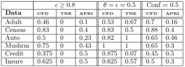
Given an error threshold², Tane searches for approximate FDs where the maximum percentage of tuples violating the FD is less than ². We run Tane with²= (1−θ). Apriori finds association rules between frequent itemsets by adding to large sets, and pruning small sets. We run Apriori using support and confidence. We use all the real datasets, and setN= 100K, n= 7 for the Census-Income dataset.

For²= (1−θ), where θranges between [0.05, 0.2], Tane returned zero dependencies across all datasets. Since Tane does not search for conditional values where partial depen-dencies may hold, it prunes candidates more aggressively and performs poorly for high² >0.5 (lowθsupport). Given these negative results, we ran Tane again using²=θ= 0.5, and 4-15 approximate FDs were returned across all datasets except the German Credit dataset (104 approximate FDs). Precision results are based on identifying dependencies that convey potentially meaningful attribute relationships (not arbitrary associations involving unique attribute val-ues). The precision results are given in Table 7, and con-sider the top-20 dependencies. The CFD precision values show that informative rules are consistently identified over Tane. For example, in the mushroom dataset, Tane dis-covers an approximate dependency of ([BRUISE, SHAPE]→

[CLR]) with a support of 50%, and while this is interesting, we are able to discover a more specific and accurate de-pendency ([CLR = ’red’, SPACE, BRUISE]→[CLS]) with support 21% that Tane was unable to find. The running times for Tane were in the order of a few seconds to less than a minute. Although our discovery times are longer (in the range of 3-14 min) the performance overhead is dominated by the larger search space. The conditional dependencies we discover are more expressive than FDs and reveal specific se-mantic relationships that FDs are not able to capture.

We ran the Apriori algorithm with the corresponding θ

support level from CFD discovery, and with confidence equal to 0.5. The Apriori algorithm runs quickly (with similar per-formance as Tane). However, it returns an unmanageably