NBER WORKING PAPER SERIES
ULTRA HIGH FREQUENCY VOLATILITY ESTIMATION
WITH DEPENDENT MICROSTRUCTURE NOISE
Yacine Aït-Sahalia
Per A. Mykland
Lan Zhang
Working Paper 11380
http://www.nber.org/papers/w11380
NATIONAL BUREAU OF ECONOMIC RESEARCH
1050 Massachusetts Avenue
Cambridge, MA 02138
May 2005
We are grateful to Joel Hasbrouck for comments and help with the sequencing of trades. Financial support from the NSF under grants SBR-0350772 (Aït-Sahalia), DMS-0204639 (Mykland and Zhang) and the NIH under grant RO1 AG023141-01 (Zhang) is also gratefully acknowledged. The views expressed herein are those of the author(s) and do not necessarily reflect the views of the National Bureau of Economic Research. ©2005 by Yacine Aït-Sahalia, Per A. Mykland, and Lan Zhang. All rights reserved. Short sections of text, not to exceed two paragraphs, may be quoted without explicit permission provided that full credit, including © notice, is given to the source.
Ultra High Frequency Volatility Estimation with Dependent Microstructure Noise
Yacine Aït-Sahalia, Per A. Mykland, and Lan Zhang
NBER Working Paper No. 11380
May 2005
JEL No. G12, C22
ABSTRACT
We analyze the impact of time series dependence in market microstructure noise on the properties
of estimators of the integrated volatility of an asset price based on data sampled at frequencies high
enough for that noise to be a dominant consideration. We show that combining two time scales for
that purpose will work even when the noise exhibits time series dependence, analyze in that context
a refinement of this approach based on multiple time scales, and compare empirically our different
estimators to the standard realized volatility.
Yacine Aït-Sahalia
Department of Economics
Fisher Hall
Princeton University
Princeton, NJ 08544-1021
and NBER
[email protected]
Per A. Mykland
The University of Chicago
[email protected]
Lan Zhang
Carnegie Mellon University
[email protected]
1
Introduction
When studyingfinancial data, the notion that noise plays an essential role is an accepted fact of life, whether at the high frequency typical of transactions data or at the lower frequencies more commonly used in asset pricing. That this is a central issue is perhaps best demonstrated by the fact that two recent presidential addresses to the American Finance Association have been entitled “noise” (Black (1986)) and “frictions” (Stoll (2000)) respectively. So we work under the assumption that the observed log-priceY (either transaction or quoted) in high frequencyfinancial data is the unobservable efficient log-priceXplus some noise component due to the imperfections of the trading process,
Yt=Xt+ t. (1.1)
SinceX is defined implicitly (as opposed to explicitly, such as the sum of expected discounted dividends for instance) the maintained identifying assumption is that is independent of the Xprocess.
We are interested in the implications of such a data generating process for the estimation of the volatility of the efficient log-price process
dXt=µtdt+σtdWt (1.2)
using discretely sampled data on the transaction price process at time intervals of length ∆. By ultra high frequency, we mean that we are in a situation where the data available are such that ∆ will be measured in seconds rather than minutes or hours. Under these circumstances, the drift is of course irrelevant, both economically and statistically, and so we shall focus on functionals of the σt process and set µt = 0. It is
the case that transactions and quotes data series in finance are often observed at random time intervals (see Aït-Sahalia and Mykland (2003) for inference under these circumstances) but, throughout this paper, we will assume for simplicity that ∆is constant. We make essentially no assumptions on theσt process: its driving
process can of course be correlated with the Brownian motionWtin (1.2), and it need not even have continuous
sample paths.
The noise term summarizes a diverse array of market microstructure effects, which can be roughly divided into three groups. First, represents the frictions inherent in the trading process: bid-ask bounces, discreteness of price changes and rounding, trades occurring on different markets or networks, etc. Second, captures informational effects: differences in trade sizes or informational content of price changes, gradual response of prices to a block trade, the strategic component of the order flow, inventory control effects, etc. Third, encompasses measurement or data recording errors such as prices entered as zero, misplaced decimal points, etc., which are surprisingly prevalent in these types of data. As is clear from the laundry list of potential sources of noise, the data generating process for is likely to be quite involved. Therefore, robustness to departures from any assumptions on is desirable.
Ifσtis modelled parametrically, we showed in Aït-Sahalia, Mykland, and Zhang (2005) that incorporating
explicitly in the likelihood of the observed log-returns Y provides consistent and asymptotically normal estimators of the parameters. But what distributional assumption to use for ? Surprisingly, we found that
misspecifying the marginal distribution of has no adverse consequences.
In the nonparametric case where σt is an unrestricted stochastic process, the object of interest is the
integrated volatility or quadratic variation of the process,hX, XiT =R0Tσ2
tdt, over afixed intervalT,typically
one day in empirical applications. This quantity can then be used to hedge a derivatives’ portfolio, forecast the next day’s integrated volatility, etc. Without noise, the realized volatility (RV) estimator [Y, Y](all)T =
Pn
i=1(Yti+1−Yti)
2 provides an estimate of the quantity hX, Xi
T, and asymptotic theory would lead one to
sample as often as possible, or use all the data available, hence the “all” superscript. The sum [Y, Y](all)T
converges to the integral hX, XiT, with a known distribution, a result which dates back to Jacod (1994) and Jacod and Protter (1998); see also e.g., Barndorff-Nielsen and Shephard (2002) and Mykland and Zhang (2002).
In Aït-Sahalia, Mykland, and Zhang (2005) and Zhang, Mykland, and Aït-Sahalia (2002), we studied the corresponding problem when a relatively simple type of market microstructure noise, iid, is present and we refer to these two papers for a review of the literature to date. We showed there that the situation changes radically in the presence of market microstructure noise. In particular, computing RV using all the data available (say every second) leads to an estimate of the variance of the noise, not the quadratic variation that one seeks to estimate: [Y, Y](all)T has bias 2nE[ 2], which is an order of magnitude larger than the object we seek to estimate, hX, XiT. The divergence of the RV estimator as the number of observations nincreases is illustrated in Figure 1, which shows the behavior of the RV estimator as a function of the sampling interval
∆=T /n: as predicted by our theory, the plot shows divergence proportional to1/n. The RV estimator in thefigure is computed for an average of the 30 Dow Jones Industrial Average stocks, averaged again over the last ten trading days in April 2004; the objective of the double averaging is to reduce the variability of the estimator in order to display its bias.
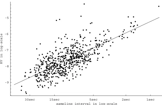
Equivalently, since our theory predicts thatRV ≈2nE£ 2¤ asymptotically inn,we expect that lnRV ≈
ln(2E£ 2¤) + lnnso that a regression oflnRV onlnnshould have slope coefficient close to1.Figure 2 shows the result: the estimated slope coefficient is1.02and the null value of 1is not rejected, with at−statistic of
0.46. Note from the equation above that an estimate ofE[ 2] can be constructed using the intercept in that regression (more on that later).
While a formal analysis of this phenomenon originated in our work cited above, the empirical message that emerges from this has long been known: do not compute RV at too high a frequency. This in fact formed the rationale for the recommendation in the literature to sample sparsely at some lower frequency. A sampling interval∆sp arse is picked in the range from5to30minutes: see e.g., Andersen, Bollerslev, Diebold, and Labys (2001), Barndorff-Nielsen and Shephard (2002) and Gençay, Ballocchi, Dacorogna, Olsen, and Pictet (2002). We denote the RV estimator corresponding to∆sparse=T /nsp arse as[Y, Y](sp arse)T .
If one insists upon sampling sparsely, we then showed in our earlier papers how to determine the optimal sparse frequency, instead of selecting it arbitrarily. But even if sampling sparsely at our optimally-determined frequency, one is still throwing away a large amount of data. For example, ifT= 1NYSE day and transactions occur every∆= 1second, the original sample size isn=T /∆= 23,400.Sampling sparsely even at the highest frequency used by empirical researchers (once every5 minutes) entails throwing away 299out of every 300
observations: the sample size used is only nsparse = 78. This violates one of the most basic principles of statistics, and our objective when starting this research project was to propose a solution which made use of the full data sample, despite the fact that ultra high frequency data can be extremely noisy.
Our approach to estimating the volatility is to use Two Scales Realized Volatility (TSRV). By evaluating the quadratic variation at two different frequencies, averaging the results over the entire sampling, and taking a suitable linear combination of the result at the two frequencies, one obtains a consistent and asymptotically unbiased estimator of hX, XiT. We start by briefly reviewing the rationale behind the TSRV estimator in Section 2.
In our earlier paper, however, we made the assumption that the noise term was iid. In Section 3, we document that dependence in the noise can be important in some empirical situations. So our main purpose in the following will be to propose a version of the TSRV estimator which can deal with such serial dependence in market microstructure noise.
Just like the marginal distribution of the noise is likely to be unknown, its degree of dependence is also likely to be unknown and so our approach will be nonparametric in nature. We develop the theory for our new, serial-dependence-robust, TSRV estimator in Section 4. In a nutshell, we will continue combining two different time scales, but rather than starting with the fastest possible time scale as our starting point, one now needs to be somewhat more subtle and adjust how fast the fast time scale is. Next, we analyze in Section 5 the impact of serial dependence in the noise on the distribution of the RV estimators,[Y, Y](all)T and[Y, Y](sparse)T . We then discuss in Section 6 a further refinement to this approach, called Multiple Scales Realized Volatility (MSRV), which achieves further asymptotic efficiency gains over TSRV (see Zhang (2004)), and as we did for TSRV and RV, we analyze the impact of serial dependence in the noise on that estimator. Finally, we provide in Section 7 an empirical study of the TSRV and MSRV estimators, and compare them to RV. We examine in particular the robustness of TSRV to the choice of the two time scales, contrast it with RV’s divergence as sampling gets more frequent and with RV’s variability in empirical samples, and study the dependence of the estimators on various ways of pre-processing the raw high frequency data. Section 8 concludes.
2
The TSRV Estimator with IID Noise
Before showing how to extend TSRV to account for serial dependence in market microstructure noise, we first review the basic TSRV construction under iid noise. The TSRV estimator is based on subsampling, averaging and bias-correction. The idea is to partition the original grid of observation times, G={t0, ..., tn}
into subsamples, G(k), k = 1, ..., K where n/K → ∞ as n → ∞. For example, for G(1) start at the first observation and take an observation every 5 minutes; forG(2), start at the second observation and take an observation every 5 minutes, etc. Then we average the estimators obtained on the subsamples. The idea is that the benefit of sampling sparsely, as in[Y, Y](sparse)T vs. [Y, Y](all)T ,can now be retained, while the variation of the estimator can be lessened by the averaging and the use of the full data sample.
Subsampling and averaging together gives rise to the estimator [Y, Y](avg)T = 1 K K X k=1 [Y, Y](sparseT ,k)
constructed by averaging the estimators[Y, Y](sparseT ,k)obtained by sampling sparsely on each of theK grids of average sizen¯.
Unfortunately,[Y, Y](avg)T remains a biased estimator of the quadratic variationhX, XiT of the true return process, although its bias2¯nE[ 2]now increases with the average sizen¯of the subsamples, instead of the full sample sizenas in2nE[ 2].ButE[ 2]can be consistently approximated by[Y, Y](all)
T : [ E[ 2] = 1 2n[Y, Y] (all) T . (2.1)
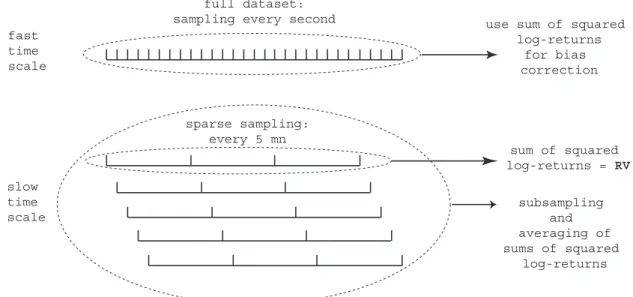
Thus a bias-adjusted estimator forhX, XiT can be constructed as \
hX, Xi(tsrv)T = [Y, Y](avg)T
| {z } slow tim e scale
− ¯nn [Y, Y](all)T
| {z } fast tim e scale
(2.2)
and this is the TSRV estimator. Figure 3 summarizes this construction.
If the number of subsamples is optimally selected asK∗=cn2/3,then TSRV has the following distribution: \ hX, Xi(tsrv)T ≈L hX, XiT | {z } ob ject of interest + 1 n1/6 [ 8 c2E[ 2]2 | {z } due to noise + c4T 3 Z T 0 σt4dt | {z } due to discretization | {z } ]1/2 total variance Ztotal (2.3)
and the constantccan be set to minimize the total asymptotic variance above.
Unlike all the previously considered ones, this estimator is now correctly centered, and to the best of our knowledge is thefirst consistent estimator forhX, XiT in the presence of market microstructure noise. A small sample refinement toh\X, XiT can be constructed as follows
\ hX, Xi(tsrv ,ad j)T =³1−n¯ n ´−1 \ hX, Xi(tsrv)T . (2.4) The difference from the estimator in (2.2) is of orderOp(¯n/n) =Op(K−1), and thus the two estimators behave
identically to the asymptotic order that we consider. The estimator (2.4), however, has the appeal of being unbiased to higher order.
Following our work, Barndorff-Nielsen, Hansen, Lunde, and Shephard (2004) have shown that our TSRV estimator can be viewed as a form of kernel based estimator. However, all kernel-based estimators are inconsis-tent estimators ofhX, XiT under the presence of market microstructure noise. When viewed as a kernel-based estimator, TSRV owes its consistency to its automatic selection of end effects which must be added “manually” to a kernel estimator to make it match TSRV. Optimizing over the kernel weights leads to an estimator with the same properties as MSRV in Section 6 below, although the optimal kernel weights will have to be found numerically, whereas the optimal weights for MSRV will be explicit (see Zhang (2004)). With optimal weights,
the rate of convergence can be improved fromn−1/6 for TSRV ton−1/4 for MSRV as the cost of the higher complexity involved in combiningO(n1/2)time scales instead of just two as in (2.2). In the fully parametric case we studied in Aït-Sahalia, Mykland, and Zhang (2005), we showed that whenσt=σis constant, the MLE
forσ2 converges forT fixed and∆→0at rate ∆1/4/T1/4 =n−1/4 (see equation (31) p. 369 in Aït-Sahalia, Mykland, and Zhang (2005)).This establishes n−1/4 as the best possible asymptotic rate improvement over (2.3).
3
Time Series Dependence in High Frequency Market
Microstruc-ture Noise
We now turn to examining empirically whether there is a need to relax the assumption that the market microstructure noise is iid. In other words, is it the case that every time a new price is observed, one observes it with an error that is independent of the previous one, no matter how close together those two successive prices might be?
3.1
The Data
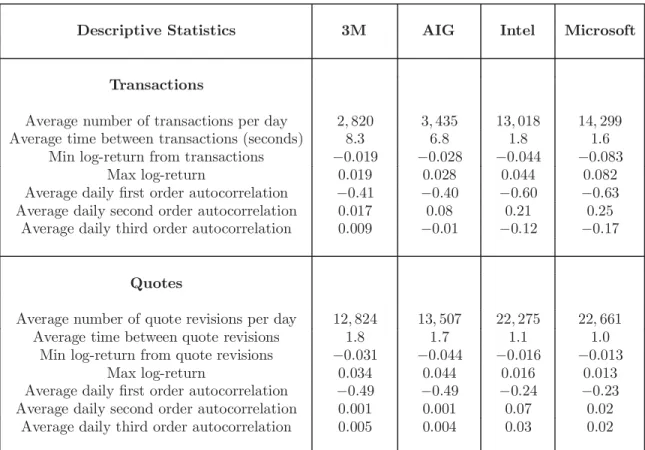
Our data consist of transactions and quotes from the NYSE’s TAQ database for the 30 Dow Jones Industrials Average (DJIA) stocks, over the last ten trading days of April 2004 (April 19-23 and 26-30). To save space, we will focus on four of the thirty stocks: 3M Inc. (trading symbol: MMM), American International Group (trading symbol: AIG), Intel (trading symbol: INTC) and Microsoft (trading symbol: MSFT). Of these, the first two are traded on the NYSE while the latter two are traded on the Nasdaq. Table 1 reports the basic summary statistics on these four stocks’ transactions.
In our earlier paper where we introduced the TSRV estimator, we assumed that microstructure noise was iid. In that case, log-returns
Yτi−Yτi−1 = Z τi
τi−1
σtdWt+ τi− τi−1 (3.1)
follow an MA(1) process since the incrementsRτi
τi−1σtdWtare uncorrelated, ⊥W and therefore, in the simple case whereσt is nonrandom (but possibly time varying),
E£¡Yτj−Yτj−1 ¢ ¡ Yτi−Yτi−1 ¢¤ = ⎧ ⎪ ⎪ ⎨ ⎪ ⎪ ⎩ Rτi τi−1σ 2 tdt+ 2E £ 2¤ ifj=i −E£ 2¤ ifj=i+ 1 0 ifj > i+ 1 (3.2)
Under the simple iid noise assumption, log-returns are therefore (negatively) autocorrelated at thefirst order. We will examine below whether this is compatible with what we observe in the data, but for now note that this is consistent with the predictions of many simple reduced form market microstructure models. For instance, in the Roll (1984) model, t= (s/2)Qt where s is the bid/ask spread andQt, the orderflow indicator, is a
in returns. French and Roll (1986) proposed to adjust variance estimates to control for such autocorrelation and Harris (1990) studied the resulting estimators. Zhou (1996) proposed a bias correcting approach based on thefirst order autocovariances; see also Hansen and Lunde (2004).
We now turn to confronting this model to the data. Figure 4 reports the autocorrelogram computed for the 3M and AIG transactions, respectively. The plot show a good agreement with the prediction of the iid noise model, namely the MA(1) structure in (3.2) for 3M and AIG.
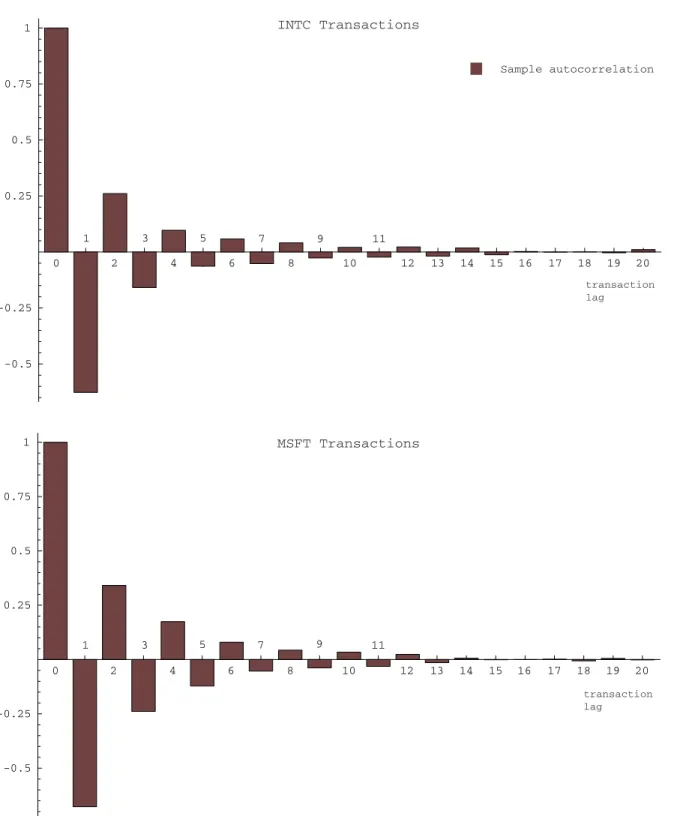
However, Figure 5 shows the corresponding result for Intel and Microsoft. It is clear that the MA(1) model, and consequently the iid noise model, does notfit those data well for these two stocks. Both stocks were added to the DJIA on November 1, 1999, becoming thefirst two companies traded on the Nasdaq to be included in the DJIA.
It is important to note however, that the difference between the twofigures does not appear to be driven by the different market structures on the NYSE (a specialist market structure) compared to the Nasdaq (a dealers’ market). In fact, the autocorrelogram pattern for the other 26 DJIA stocks is closer to that of Intel and Microsoft, not that of 3M and AIG. Table 2 reports the results of a cross-sectional OLS regressions of the autocorrelation coefficients of order 2-5 on the average time between transactions used as a measure of the liquidity of the stock, for the 30 DJIA stocks. These autocorrelation coefficients of order greater than 1 would be zero if the noise term were serially uncorrelated, as in (3.2). The table shows that the lower the time between successive transactions, the higher the observed autocorrelation in absolute value (the coefficients alternate signs because the autocorrelation coefficients do, as in Figure 5). In other words, based on these data, the more liquid the stock, the more likely we are to face departures from the iid assumption.
3.2
Example: A Simple Model to Capture the Noise Dependence
A simple model to capture the higher order dependence that we just documented in INTC and MSFT trades is
ti =Uti+Vti (3.3)
whereU is iid,V isAR(1) withfirst order coefficientρ,|ρ|<1,andU ⊥V.Under this model, we have
E£¡Yτj−Yτj−1 ¢ ¡ Yτi−Yτi−1 ¢¤ = ⎧ ⎪ ⎪ ⎨ ⎪ ⎪ ⎩ Rτi τi−1σ 2 tdt+ 2E £ U2¤+ 2 (1−ρ)E£V2¤ ifj =i −E£U2¤−(1−ρ)2 E£V2¤ ifj=i+ 1 −ρj−i−1(1−ρ)2E£V2¤ ifj > i+ 1 (3.4)
This model can easily befitted to the data by the generalized method of moments. We use thefirst twenty autocovariances of the log-returns as moment functions, in order to estimate the three parameters E[U2], E[V2]andρ. Their estimated values are4.2 10−8,3.5 10−8 and−0.68 for INTC and2.9 10−8,4.3 10−8 and
−0.70for MSFT. Figure 6 shows the sample autocorrelogram and the corresponding onefitted by the model above.
Let us stress, however, that, while this simple model seems to capture fairly well the dependence in the stock data that we have examined, our theory is not tied to this particular specification. of . It applies to
fairly general dependence structures, as can be seen from Assumption 1 below.
3.3
Transactions or Quotes?
The model (3.3) for the microstructure noise describes well a situation where the primary source of the noise beyond order one consists of further bid-ask bounces. In such a situation, the fact that a transaction is on the bid or ask side has little predictive power for the next transaction, or at least not enough to predict that two successive transactions are on the same side with very high probability (although Choi, Salandro, and Shastri (1988) have argued that serial correlation in the transaction type can be a component of the bid-ask spread, and extended the model of Roll (1984) to allow for it).
Figure 5 and the estimates just reported (ρ=−0.7) are evidence of negative autocorrelation at horizons of up to about15transactions. In trying to assess the source of the higher order dependence in the log-returns, a natural hypothesis is that this is due to the trade reversals: in transactions data and an orderly liquid market, one might expect that in most cases successive transactions of the same sign (buy or sell orders) will not move the price. The next recorded price move is then, more likely than not, going to be caused by a transaction that occurs on the other side of the bid-ask spread, and so we observed these reversals when the data consist of the transactions that lead to a price change.
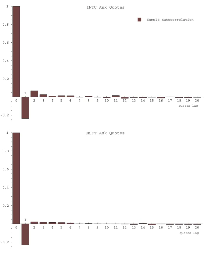
To examine this hypothesis, we turn to quotes data, also from the TAQ database. The results are reported in Figure 7 and suggest that an important source for the AR(1) pattern with negative autocorrelation (the termV in (3.3)) will be trade reversals. The remaining autocorrelation exhibited in the quotes data can also be captured by model (3.3), but with a positive autocorrelation in theV term. This can capture effects such as the gradual adjustment of prices in response to a shock such as a large trade.
4
Extending the TSRV Estimator for Dependent Noise
In the previous section, we found that there are empirical situations (such as Intel or Microsoft transactions) where the assumption of iid market microstructure noise could be problematic. We now proceed to suitably extending the TSRV estimator to make it robust to departures from the iid noise assumption. The idea is to somewhat slow the fast time scale to reduce the degree of dependence that is induced by the noise.
4.1
The Setup
As above, we let Y be the logarithm of the transaction price, which is observed at times 0 = t0, t1, ... , tn = T. We assume that at these times, Y is related to a latent true price X (also in logarithmic scale)
through equation (1.1). The latent priceX is given by (1.2).
Assumption 1. We assume that the noise process ti is independent of theXt process, and that it is (when
viewed as a process in indexi) stationary and strong mixing with the mixing coefficients decaying exponentially. We also suppose that for someκ >0,E 4+κ<∞.
Definitions of mixing concepts can be found e.g., in Hall and Heyde (1980), p. 132. Note that by Theorem A.6 (p. 278) of Hall and Heyde (1980), there is a constantρ <1so that, for all i,
¯
¯Cov( ti, ti+l)
¯
¯ ≤ ρlVar( ) (4.1)
For the moment, we focus on determining the integrated volatility ofX for one time period[0, T]. This is also known as the continuous quadratic variationhX, XiofX. In other words,
hX, XiT =
Z T
0
σ2tdt. (4.2)
Our volatility estimators can be described by considering subsamples of the total set of observations. A realized volatility based on everyj’th observation, and starting with observation numberr, is given as
[Y, Y](Tj,r)= X
0≤j(i−1)≤n−r−j
(Ytji+r−Ytj(i−1)+r)
2 .
Under most assumptions, this estimator violates the sufficiency principle, whence we define theaverage lag j realized volatility as [Y, Y](TJ)= 1 J J−1 X r=0 [Y, Y](TJ,r) = 1 J nX−J i=0 (Yti+J −Yti) 2 (4.3)
A generalization of TSRV can be defined for1≤J < K ≤nas \
hX, Xi(tsrv)T = [Y, Y](TK)
| {z } slow tim e scale
−n¯n¯K J
[Y, Y](TJ)
| {z } fast tim e scale
, (4.4)
thereby combining the two time scales J andK. Heren¯K = (n−K+ 1)/K and similarly forn¯J.
We will continue to call this estimator the TSRV estimator, noting that the estimator we proposed in Zhang, Mykland, and Aït-Sahalia (2002) is the special case whereJ = 1andK→ ∞asn→ ∞. The original TSRV produces a consistent estimator in the case where the ti are iid. For the optimal choiceK=O(n
2/3), \
hX, Xi(tsrv)T −hX, XiT =Op(n−1/6).
The problem with which we are concerned here is that these assumptions on the noise timay be too restrictive.
We shall see that in the case where J is allowed to be larger than1, the problem of dependence of the ti’s
will be eliminated and the generalized TSRV estimator given in (4.4) will be consistent for suitable choices of
(J, K).
4.2
A Signal-Noise Decomposition
Lemma 1. Under the assumptions above, letn→ ∞, and letj=jn be any sequence. Then nX−j
i=0
(Xti+j −Xti)( ti+j − ti) =Op(j
1/2).
The lemma is important because it gives rise to the sum of squares decomposition
[Y, Y](TJ)= [X, X](TJ)+ [ , ](TJ)+Op(J−1/2).
Thus, if we look at linear combinations of the form (4.4), one obtains \ hX, Xi(tsrv)T = [X, X](TK)−¯nK ¯ nJ [X, X](TJ) | {z } sign al term + [ , ](TK)−n¯K ¯ nJ [ , ](TJ) | {z } n oise term + Op(K−1/2), so long as 1≤J≤K and K=o(n), (4.5)
both of which will be assumed throughout.
4.3
Analysis of the Noise Term
It can be seen that when the ’s are independentE[noise term] = 0, so that the linear combination used in (4.4) is exactly what is needed to remove the bias due to noise. To analyze the more general case, and to obtain approximate distribution of the noise term, note that
[ , ](TJ)= 1 J n X i=0 c(iJ) 2ti−2 J nX−J i=0 ti ti+J, (4.6)
wherec(iJ)= 2forJ≤i≤n−J, and= 1 for otheri. By construction X i c(iJ)= 2Jn¯J, (4.7) so that E|noise term|≤2E 2 µ 1 K(n−K+ 1)ρ K+¯nK ¯ nJ 1 J(n−J+ 1)ρ J ¶ =O³n K(ρ K+ρJ)´ (4.8)
and, in the regular case whereCov( t0, tk) =o(Cov( t0, tJ))
E[noise term] = 2E 2n
KCov( t0, tJ)(1 +o(1)).
IfJ → ∞at even a quite slow rate whenn→ ∞, the bias is negligible. Also, in the case of m-dependent s, the bias becomes zero forfiniteJ. We obtain:
Proposition 1. Under assumption (4.13) below,
K
n1/2 (noise term−E[noise term]) L
−→ξZn o is e (4.9)
asn→ ∞, where Zn o ise is standard normal. Further, in the case where both J andK go to infinity with n,
we have thatξ2=ξ2 ∞, where ξ∞2 = 16 Var( )2+ 32 ∞ X i=1 Cov( t0, ti) 2. (4.10)
In the case whereJ does not go to infinity (the m-dependent case, say), then
ξ2=ξ∞2 + 8 ∞ X i=−∞ Cov( ti−J, ti+J) 2+ 8 X∞ i=−∞ Cum( t0, ti, tJ, ti+J), (4.11)
Note that even whenJ→ ∞, one may be better offusing (4.11) thanξ2∞since the former is closer to the small sample variance, and sinceJ → ∞quite slowly. (By contrast, K→ ∞much more quickly, as we shall see).
4.4
Analysis of the Signal Term
As for the “signal term”, we obtain that
[X, X](TK)→hX, XiT (4.12)
in probability as n → ∞, provided K = o(n). Obviously, for the signal term in h\X, XiT −hX, XiT to be scalable to be consistent (see equation (4.17) below), we need
lim sup n→∞
J
K < 1, (4.13)
which is easily satisfied. In fact, as we shall see, one would normally take
lim sup n→∞
J
K = 0. (4.14)
Specifically, we have in the case of dependent noise:
Proposition 2. Under (4.5), µK n µ 1 + 2J 3 K3 ¶¶−1/2µ [X, X](TK)−¯nK ¯ nJ [X, X](TJ)−hX, XiT ¶ L −→η√T Zd iscrete, (4.15)
where, Zdiscrete is standard normal, and where in general, η2 is given as the limit in Theorem 3 in Zhang,
Mykland, and Aït-Sahalia (2002) (i.e., the discretization variance η2 has the same expression as when the
noise is iid). In the special case where observations are equidistant,
η2= 4 3
Z T
0
The convergence in law is stable (see Chapter 3 of Hall and Heyde (1980)), the most important consequence of which is thatZdiscrete is independent ofη.
4.5
The Combined Estimator
Consider the adjusted estimator \ hX, Xi(tsrv ,ad j)T = µ 1−n¯K ¯ nJ ¶−1 \ hX, Xi(tsrv)T (4.17) In the iid case of Zhang, Mykland, and Aït-Sahalia (2002), this adjustment was introduced from small sample considerations (Section 4.2). Here, we also see that in the case where (4.13) is satisfied but (4.14) is not, this adjustment is needed for consistency. In the following, we analyze this estimator, and for the case when (4.14) holds, the same analysis applies to the originalh\X, Xi(tsrv)T .
We obtain from equations (4.9) and (4.15) that \ hX, Xi(tsrv ,adj)T = à 2E 2n KCov( t0, tJ) + n1/2 K ξZnoise + µ K n µ 1 + 2J 3 K3 ¶¶1/2 η√T Zdiscrete ! × µ 1−n¯K ¯ nJ ¶−1 (1 +op(1)), (4.18)
whereZn oise andZd iscrete are asymptotically standard normal, and asymptotically independent.
It is easy to see that the optimal trade-offbetween the two variance terms results in a choice ofK=O(n2/3). The worst thing that can then happen to the bias term is then that this is of the order of(n/K)ρJ =n1/3ρJ.
Thus the bias is of small order relative to the variance provided one choosesn1/3ρJ =o(n−1/6), i.e., ρJ =
o(n−1/2). Thus, one can safely assume thatJ/K∼0(i.e., (4.14)), and it follows that
Proposition 3. The asymptotic behavior of the estimatorh\X, Xi(tsrv,ad j)T is given by
\ hX, Xi(tsrv,ad j)T = Ã 2¡E 2¢ n KCov( t0, tJ) + n1/2 K ξZn oise+ µ K n ¶1/2 η√T Zd iscrete ! (1 +op(1)). (4.19)
Thus the optimalKis as given above, and one chooses, ultimately,J so that
Cov( t0, tJ) =o(n−
1/2). (4.20)
Obviously, when is m-dependent, one can simply chooseJ =m+ 1.
4.6
A Further Adjustment to the TSRV Estimator
It should be noted that whenKis large,[X, X](TK)may be a slight underestimate ofhX, XiT. To consider the issue, ifσ2
t is constant,σ2t =σ2, one gets thathX, XiT =σ2T, whereas[X, X]
(K)
approximation here is loose, but, for example, it is an equality in expectation whenσ2 t is constant). Thus [X, X](TK)−n¯K ¯ nJ [X, X](TJ)≈σ2T µ n−K+ 1 n − ¯ nK ¯ nJ n−J+ 1 n ¶ =σ2T(K−J)¯nK n . (4.21)
A further modification of our estimator is thus the area adjusted quantity \ hX, Xi(tsrv ,aa)T = n (K−J)¯nK \ hX, Xi(tsrv)T . (4.22) Since, by (4.5), n (K−J)¯nK ∼ µ 1−¯nK ¯ nJ ¶−1 (4.23) we have:
Proposition 4.The estimatorh\X, Xi(tsr v,a a)T has the same asymptotics ash\X, Xi(tsrv,ad j)T given in Proposition 3.
In conclusion, the TSRV estimator that is robust to serial dependence in the noise, behaves as follows: \ hX, Xi(tsrv,aa)T ≈L hX, XiT + 1 n1/6 [ 1 c2ξ 2 | {z } due to noise + c4T 3 Z T 0 σ4 tdt | {z } du e to d iscretization | {z } ]1/2 total varian ce Ztotal (4.24)
whether it is taken in the formh\X, Xi(tsrv,aa)T orh\X, Xi(tsrv ,ad j)T . HereK∼cn2/3, andξis given by (4.10), or, more generally, (4.11).
5
RV Under Serial Dependence in the Noise
We now turn to an analysis of the standard RV estimator when the noise is serially dependent. First, we have than sparse sampling at a givennsparse results in the same asymptotic distribution as when the noise is serially uncorrelated. Second, however, wefind that dependence in the noise impacts the asymptotic variance (but not the bias) of the RV estimator when all the data (alln) are used. Specifically:
Proposition 5.The traditional RV estimator,[Y, Y](spar se)T ,computed at a sparse sampling frequency∆spa rse = T /nspa r se,has the following behavior:
[Y, Y](spa rse)T ≈L hX, XiT + 2ns pa rs eE 2 | {z } bias du e to n oise + [4nspar seE 4 | {z } due to n o ise + 2T nspar se Z T 0 σt4dt | {z } du e to d iscretiz atio n | {z } ]1/2 to ta l va ria n ce Ztotal. (5.1)
The reason why this last expression is as in the iid case is as follows. Essentially, the asymptotic variance ofPi ti ti+J behaves as if the quantities were uncorrelated ifJ goes to infinity, and so when we havensp arse =
n/J go to infinity with n effectively the log-returns involved in [Y, Y](sp arseT ) are separated by enough time interval for the dependence in not not to matter. Then Pi ti
¡ ti+J−E £ ti+J|Fi ¤¢ is a martingale, with variance PiEh 2ti¡ ti+J−E £ ti+J|Fi ¤¢2i
, which is approximately nsparseE£ 2¤ 2
under exponential mixing, while the remainder termPi ti
¡
ti+J−E
£
ti+J|Fi
¤¢
becomes negligible under exponential mixing.
By contrast, when all the observations are used, as in[Y, Y](all)T ,the asymptotic variance of RV is influenced by the dependence of the noise. The asymptotics of[Y, Y](all)T are, to first order, like that of[ , ]. The mean of the latter is 2nE 2. As for the asymptotic variance, from standard formulas for mixing sums, we have
Ω∞= AVAR ∙√ n µ[ , ] n −2E 2 ¶¸ = Var(( 1− 0)2) + 2 ∞ X i=1 Cov((1− 0)2,( i+1− i)2). (5.2) This gives:
Proposition 6. By contrast, the RV estimator using all the data,[Y, Y](al l)T ,computed at the highest sampling frequency∆=T /n, has the following behavior:
[Y, Y](a ll)T ≈L hX, XiT + 2| {z }nE 2 bia s d ue to n o ise + [ 4n Ω∞ | {z } d ue to n o is e + 2T n Z T 0 σt4dt | {z } d ue to discretization | {z } ]1/2 tota l va rian ce Zto ta l. (5.3)
whereΩ∞=E 4 when the noise is iid; otherwise, dependency in gives rise toΩ
∞ in (5.2).
An alternate expression forΩ∞can be obtained by noting that
Cov(( 1− 0)2,( i+1− i)2) = 2 Cov( 1− 0, i+1− i)2+ Cum( 1− 0, 1− 0, i+1− i, i+1− i)
(and similarly for the variance).
6
MSRV: Multiple Scales Realized Volatility
We have seen that TSRV provides thefirst consistent and asymptotic (mixed) normal estimator of the quadratic variationhX, XiT,that it can be made to work even if market microstructure noise is serially dependent, and that it has the rate of convergencen−1/6. At the cost of higher complexity, it is possible to generalize TSRV to multiple time scales, by averaging not on two time scales but on multiple time scales. The resulting estimator,
multiple scale realized volatility (MSRV), has the form of \ hX, Xi(m srv)T = XM i=1 ai [Y, Y] (Ki) T | {z }
weighted su m ofM slow tim e scales
+ 2 Ed2
|{z} fast tim e scale
. (6.1)
For suitably selected weights ai’s, h\X, Xi
(m srv)
T converges to the true hX, XiT at rate n−1/4. In what
follows, we recall the construction of the MSRV estimator in the iid case (see Zhang (2004)), before making it robust to time series dependence in market microstructure noise of the same type we assumed in the above analysis of TSRV (see Assumption 1).
6.1
A Signal-Noise Decomposition
To describe the selection of the weightsai’s, we start with a special case, where we restrict attention to weights
that satisfy the two conditions
XM i=1ai= 1, (6.2) XM i=1 ai Ki = 0. (6.3)
Then under (6.3), we have the decomposition \ hX, Xi(m srv)T = M X i=1 ai[X, X](TKi) | {z } sign al + M X i=1 aiUn,Ki | {z } n oise + 2 M X i=1 ai[X, ](TKi) | {z }
signal-n oise interaction
+ M X i=1 aiEn,Ki+ 2E 2 | {z }
end p oints of noise
+ Op(n−1/2), (6.4) where Un,K =− 2 K n X i=K ti ti−K, and En,K=− 1 K KX−1 j=0 2 tj− 1 K n X j=n−K+1 2 tj.
Condition (6.2) ensures that thefirst term in (6.4) will be asymptotically unbiased forhX, XiT.
6.2
Analysis of the Noise Term
Consider the noise term in (6.4)
ζ= M
X
i=1
aiUn,Ki (6.5)
SinceUn,Ki andUn,Kl are uncorrelated zero-mean martingales, under conditions (6.2)-(6.3),
forKi<< n, where γ2= 4 M X i=1 µ ai Ki ¶2 .
Subject to conditions (6.2)-(6.3), one canfind the optimal weightsai,i= 1, ..., M,so that (6.6) is minimized.
In the special case whereKi=i, the optimal weighta∗i is given by
a∗i = 12 i M2 ¡ i M − 1 2− 1 2M ¢ ¡ 1−M12 ¢ . And the resulting variance of the noise term is minimized at
Var∗(ζ) = 48n
M(M2−1)(E
2)2 (6.7)
6.3
Analysis of the Signal Term
The signal term in (6.4) is
φ= M
X
i=1
ai[X, X](Ti). (6.8)
Let the lagJ discretization error be[X, X]T(J)−hX, XiT.Unlike the noise term, the signals at different lags are highly correlated. In particular, the covariance between the lagJ and lagK discretization error is,
ΥJ,K = T n(min(J, K)−1) 2 3 µ 3−min(J, K) + 1 max(J, K) ¶ η2 (6.9)
where, when theti are equidistant, and under regular allocation of points to subgrids,
η2= 2
Z T
0
σ4tdt. (6.10)
It is straightforward from (6.9) that
φ−hX, XiT =Op((n/M)−1/2). (6.11)
The interaction termPMi=1ai[X, (Ki)]T and the end points of noise are of orderM−1/2. Hence, after balancing
the terms in (6.4), one obtains the optimalM is
M=O(n1/2). (6.12)
Therefore, the rate of convergence for the overall error for MSRV is \
hX, Xi(m srv)T − hX, XiT = Op(n−1/4), (6.13)
which is an improvement over TSRV’s \
at the cost of course of the greater complexity of MSRV over TSRV. As discussed above, from our earlier analysis of the parametric case, the raten−1/4 is optimal.
6.4
Noise-Optimal Weights
Consider now the larger class of weights ai= i M2h µ i M ¶ −2M12 i Mh 0 µ i M ¶ , (6.15)
wherehis a continuously differentiable real-value function with derivativeh0,and satisfying the following two conditions: Z 1 0 xh(x)dx= 1, (6.16) Z 1 0 h(x)dx= 0. (6.17)
This class of weights encompassed the earlier class (6.2)-(6.3). When the weights are chosen optimally,htakes the form
h∗(x) = 12 µ x−1 2 ¶ (6.18) and the general optimal weights are then
a∗ i = i M2h∗ µ i M ¶ − i 2M3h∗0 µ i M ¶ . (6.19)
Using the optimal choiceh∗, the asymptotic variance forh\X, Xi(m srv)
T is Υ |{z} total variance = 48c−3(E 2)2 | {z } du e to n oise + 52 35cT η 2 | {z } d ue to discretization (6.20) + 12 5c− 1Var( 2) | {z }
due to noise end p oints
+ 48
5c−
1E 2hX, Xi
T
| {z }
d ue to interaction b etweenXand
wherecis the proportionality constant inM =cn1/2.
To summarize, when computed the optimal weights (6.19), the MSRV estimator has the following distrib-ution: \ hX, Xi(m srv)T ≈L hX, XiT + 1 n1/4 h Υ |{z} i1/2 total variance Ztotal (6.21) when using the optimal weights (6.18). We can then select the value of the constant c to minimize the asymptotic variance in the expression (6.21). Notefinally that this class of weights is optimal for the purpose of minimizing the part of the asymptotic distribution that is due to the presence of the noise. There is room
for achieving further small asymptotic gains by minimizing over the full asymptotic variance (only at the level of the constant and not the rate, which is already optimal here) but at the cost of even greater complexity resulting in the loss of the simple, explicit, selection rule (6.19) for the weights.
6.5
The AVAR of MSRV When the Noise is Serially Dependent
We now study the MSRV estimator under the (dependence) Assumption 1 from Section 4.1. The only extra bias (due to dependency) in equation (6.4) comes from theUn,Ki. Under our mixing assumption,
|E[Un,Ki]| ≤ 2 KVar( ) n X j=Ki ρi ≤ 2 KVar( ) ρKi 1−ρ Thus, when theai follow (6.15), the absolute value of the extra bias in (6.4) becomes
¯ ¯ ¯¯ ¯E "M X i=1 aiUn,i #¯¯ ¯¯ ¯ ≤ M X i=1 2 M2 ¯ ¯ ¯ ¯h(Mi ) ¯ ¯ ¯ ¯ ρ i 1−ρ+correspondingh 0 term =O(M−1) (6.22)
To the extent that the MSRV estimator converges at the rateOp(M−1/2), the bias induced by the dependence
of the ’s is therefore irrelevant asymptotically.
An inspection of the terms in (6.4) shows that the rate of convergence does, indeed, remain of order Op(M−1/2) =Op(n−1/4)under Assumption 1. As in the TSRV case, however, the asymptotic (random)
vari-ance now changes due to the dependence of the ’s. To compute that varivari-ance when the market microstructure noise is serially dependent, notefirst that the four terms in (6.4) are asymptotically independent. This is by the same methods as we use in the following. Also, the behavior of the signal term is, obviously, unchanged.
We compute the covariances of the individual terms, and obtain:
Proposition 7. The overall (random) asymptotic variance ofh\X, Xi(m s rv)T −hX, XiT is given, in the presence of (possibly) serially correlated noise with autocorrelation functionγ(l) = Cov( 0, tl),by:
M4 3T η 2Z 1 0 dx Z x 0 h(y)h(x)y2(3x−y)dy + 1 M4 M X J=1 M X K=1 h(J M)h( K M)hX, XiT K X l=−J (γ(l) +γ(l+J−K)−γ(l−K)−γ(l+J))(min(l+J, K)−max(0, l)) + 4 M4 M X J=1 M X K=1 h(J M)h( K M) nX−J l=−(n−K)
(min(n, n+l)−max(J+l, K) + 1)+Cov( t0 t−J, tl tl−K) (6.23)
+ 2 M4 M X J=1 M X K=1 h(J M)h( K M) KX−1 l=−(J−1)
(min(J+l, K)−max(0, l) + 1)+Cov( 2t0, 2tl).
For example, in the special case of model (3.3), we have γ(l) = ⎧ ⎪ ⎪ ⎨ ⎪ ⎪ ⎩ 2E£U2¤+ 2 (1−ρ)E£V2¤ ifl= 0 −E£U2¤−(1−ρ)2E£V2¤ if|l|= 1 −ρ|l|−1(1−ρ)2 E£V2¤ if|l|>1 (6.24)
to be inserted in (6.23). It can also be noted that, if instead
γ(l) = ⎧ ⎪ ⎪ ⎨ ⎪ ⎪ ⎩ 2E£U2¤ ifl= 0 −E£U2¤ if|l|= 1 0 if|l|>1 (6.25)
then the expression (6.23) reduces to the asymptotic variance of MSRV in the iid case, that isΥin (6.20). We conclude our analysis of MSRV with two remarks:
Remark 1. Recall that for TSRV we replaced (2.2) with (4.4), thereby “jumping” to frequencies (J, K)over the very fastest one (1, K) at which the serial dependence in the noise manifests itself. By letting both J
andK go to infinity with n, we were effectively able to eliminate the serial dependence within each subgrid. However, the asymptotic variance of TSRV is affected by the serial dependence across subgrids coming from the averaging over RV from different subgrids in both [Y, Y]T(K) and [Y, Y](TJ) in (4.4), hence the asymptotic variance in Proposition 3, also in (4.24), which is different than in the iid noise case.
Remark 2. The asymptotic distribution of MSRV is also affected by the dependence of the noise. Unlike the TSRV case, there is no benefit to adjusting the MSRV estimator in the presence of serial dependence in the noise. This is because the weights a∗
i in (6.19) already assign most of the mass on the interval [1, M] with
M =O(n1/2) to subintervals of the form[cM, M] where cis a positive constant. Therefore, the very fastest
frequencies of observations (those close tom= 1)already play a small role in MSRV even under iid noise.
7
Empirical Analysis
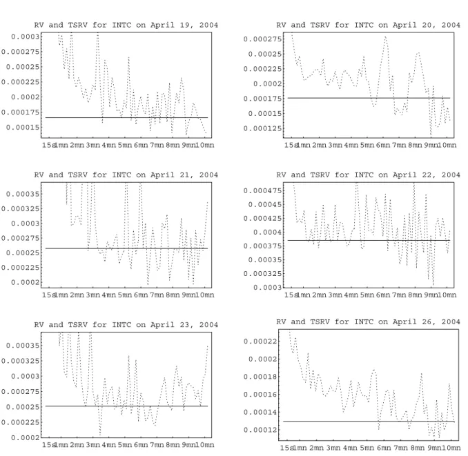
With these theoretical results in hand, we now turn to a comparison of the empirical performance of the RV, TSRV and MSRV estimators, study the impact of the selection of the fast and slow time scales on the TSRV estimators and the improvement due to MSRV relative to TSRV in the context of transactions data for Intel and Microsoft in the last ten days of April 2004.
7.1
Comparison of the RV and TSRV Estimators
In our empirical analysis of the different estimators, we start by comparing our TSRV estimator to the traditional RV estimator. In particular, we establish that TSRV solves the two main problems associated with RV, namely the divergence of RV as the sampling interval gets small and the variability of RV. The comparison is reported for Intel in Figure 8 and for Microsoft in Figure 9, where we compare RV computed at different sampling frequencies with TSRV.
Besides the well-known divergence of RV as∆→0,the twofigures also demonstrate the large difference in variability of both estimates. Without the benefits of the double averaging in Figure 1, what these two series of plots show is that computing RV at, say,4mn as opposed to5mn or6mn can result in substantially different daily estimates. And the computation of day-by-day estimates is how RV is actually used. In existing empirical applications, RV has typically been employed in the empirical literature at an arbitrary sparse frequency: in light of the variability of RV as a function of the sparse sampling interval∆sparse,whatever particular choice is made can matter.
7.2
Robustness of TSRV to the Choice of Slow Time Scale
Both RV and TSRV require that the econometrician make a choice. In RV, one needs to select the sparse sampling frequency at which to compute the estimator. In TSRV, one needs to select the number of subgrids K over which to average the slow time scales sum of squares. In Zhang, Mykland, and Aït-Sahalia (2002), we showed how to compute an optimal value K∗ for the slow time scale parameter K when the noise term
is assumed to be iid, but in practical application it would be beneficial to be able to dispense with that computation. For that, we would need to establish that the TSRV estimator is empirically robust to departures from the optimalK∗.So, we now examine and compare the robustness of the two estimators to the selection
of their respective free parameter.
The left panels in Figure 10 show RV, computed for Intel and Microsoft, as an average of the RV values over the last ten days in April 2004 for different sparse sampling frequency (which is the choice parameter for RV). The right panels report the robustness of TSRV to the choice ofK. The right panels show that the estimator is numerically very robust to a large range of choices ofK.In other words, the value of the TSRV estimator is largely unaffected by choice ofK within a reasonable range.
7.3
Robustness of TSRV to the Choice of Slow and Fast Time Scales
When the noise is serially dependent, the TSRV estimator defined in (4.4) depends on the choice of both the slow time scale(K)and the fast time scale(J).Wefind that the time-dependent TSRV is quite robust to the choice of(J, K).Figure 11 shows that the value of the estimator is essentially identical within the reasonable range of values considered.
7.4
The Improvement in MSRV over TSRV
It is possible to improve upon TSRV by considering MSRV. Both are consistent estimators ofhX, XiT,but MSRV has the faster convergence rate n−1/4 vs. n−1/6 for TSRV. The trade-off involves the additional computational burden, since the number of slow time scales to be computed for MSRV is M =O(n1/2) and n can be large in empirical applications: for instance n= 23,400 for a stock that trades on average once a second for a full day.
We now examine the difference between TSRV and MSRV in the context of our empirical application. Figure 12 shows that both methods produce close .estimates, especially when compared to the differences
exhibited earlier between RV and TSRV. As in the case of TSRV shown in 11, the MSRV estimator is not sensitive to the specific choice ofM within a reasonable range.
7.5
Robustness to Data Cleaning Procedures
One aspect that is sometimes briefly mentioned, but often not emphasized, in empirical papers using high frequency financial data is the fact that the raw data is typically pre-processed to eliminate data errors, outliers, etc. In addition, empirical applications of RV can involve pre-filtering of the data of various types, but we focus here on the impact of data cleaning procedures that typically take place before any actual RV computation is performed.
It turns out that the impact of the specific data-cleaning procedures used to pre-process the raw data can have a large impact on RV estimators. We illustrate this effect by considering different cutoffs to determine which outliers to eliminate before calculating the RV estimator. First, we eliminate the obvious data errors (such as a transaction price reported as zero, transaction times that are out of order, etc.).
Second, we seek to eliminate outliers of various sizes. This is where things get trickier. For that purpose, an outlier is a “bounceback”: a log-return from one transaction to the next that is both greater in magnitude than an arbitrary cutoff, and is followed immediately by a log-return of the same magnitude but of the opposite sign, so that the price returns to its starting level before that particular transaction. Certainly, we do not expect such large “roundtrips” to represent meaningful transactions. The question is how large is large, and so we are led to study the dependence of the RV and TSRV estimators on three different cutoffs that could conceivably be adopted, 0.1% and 1% respectively in log-returns terms, and no cutoff (no raw bounceback return is larger than 2% in our sample, so that any cutoff larger than this would make no difference). The analysis reported above is all based on the intermediary cutoffof1%.
The left panels in Figure 13 show the large impact of the cutoff on the RV estimator. As shown in the right panel, where all three curves are close together, TSRV is much less sensitive to the specific cutoffused. This is due to the structure of TSRV as a difference of two estimators: large returns in the data are part of the slow time scale calculation, but then subtracted out in the fast time scale one.
Since the cutofflevel is essentially arbitrary, we can view such outliers as a form of market microstructure noise, and the robustness of TSRV to different ways of pre-processing the data is therefore a desirable property.
8
Conclusions
We documented that there are instances where the market microstructure noise contained in high frequency financial data can exhibit serial correlation. We showed that combining two or more time scales for the purpose of estimating integrated volatility will work even in the situation where the microstructure noise exhibits time series dependence.
In most data error situations, one might expect that progress will lead the issue to become somehow less salient over time. But in this instance, the measurement errors we face in ultra high frequency data are compounded by the institutional evolution of the equity markets. While changes such as the passage to
decimalization contribute to reducing the amount of noise in the data, by reducing the rounding errors, the emergence of competing electronic networks means that multiple transactions can be executed (and ultimately reported in our database) on different exchanges at the same time, thereby increasing the potential for slight time reporting mismatches and other forms of data error.
Indeed, the data generated by the individual market venuesfind their way to the public in various ways. The principal Electronic Communication Networks (ECNs), such as INET and its precursors and Archipelago, have high speed dissemination directly to their subscribers. These dissemination systems run on a telecom-munications protocol known as “frame relay”, which is quite fast. Most other market data, however, reaches the trading public (and ultimately us econometricians) either through Nasdaq’s dissemination or CTS/CQS. The Consolidated Tape Association administers the CTS (the consolidated trade system) and CQS (the con-solidated quote system). Virtually all US trades are reported to CTS, but the path may be indirect. Island (not INET) may report a trade to the National (formerly Cincinnati) Stock Exchange, which will then report it to CTS, which then broadcasts it to us. The general problem is that trading activity is fast relative to the CTS speed of collection and dissemination.
Furthermore, Nasdaq has had long-standing issues with late and delayed trade reports. In principle, a Nasdaq member has up to 30 (in the past, 90) seconds to report a trade and anecdotal evidence suggests that some dealers were/are using this leeway to its greatest extent. Since this practice was not uniform across dealers and across time, the sequencing can be suspect. And the sequencing across exchanges may be unreliable over very short time intervals: a trade on one exchange followed (and time-stamped to the same second as) a trade in the same stock on a different exchange, may not in fact have occurred in that order.
While the consolidated tape feed (which we see on TAQ) is probably the best source of data available, we may not be seeing the trades in the order in which they occurred, and the emergence and further development of alternative networks on which to trade the same stocks makes the issue of market microstructure noise in the data an increasing, not decreasing, one. ECNs represent over 30% of Nasdaq trading volume and are increasing their market share in NYSE-listed issues as well (see e.g., Barclay, Hendershott, and McCormick (2003)). Clearly, the decentralization of trading, combined with the increased frequency of trading, create challenges for the data collection which ultimately affect the estimation of a quantity as basic as the daily integrated volatility of the price. So there are reasons to believe that the issue of controlling for market microstructure noise in high frequencyfinancial econometrics will be with us for some time.
References
Aït-Sahalia, Y., and P. A. Mykland (2003): “The Effects of Random and Discrete Sampling When Estimating Continuous-Time Diffusions,” Econometrica, 71, 483—549.
Aït-Sahalia, Y., P. A. Mykland, and L. Zhang (2005): “How Often to Sample a Continuous-Time Process in the Presence of Market Microstructure Noise,”Review of Financial Studies, 18, 351—416.
Andersen, T. G., T. Bollerslev, F. X. Diebold,andP. Labys(2001): “The Distribution of Exchange Rate Realized Volatility,”Journal of the American Statistical Association, 96, 42—55.
Barclay, M. J., T. Hendershott, andD. T. McCormick(2003): “Competition among Trading Venues: Information and Trading on Electronic Communications Networks,”Journal of Finance, 58, 2637—2665.
Barndorff-Nielsen, O. E., P. R. Hansen, A. Lunde,andN. Shephard(2004): “Regular and Modified Kernel-Based Estimators of Integrated Variance: The Case with Independent Noise,” Discussion paper, Department of Mathematical Sciences, University of Aarhus.
Barndorff-Nielsen, O. E., and N. Shephard(2002): “Econometric Analysis of Realized Volatility and Its Use in Estimating Stochastic Volatility Models,”Journal of the Royal Statistical Society, B, 64, 253—280.
Black, F.(1986): “Noise,”Journal of Finance, 41, 529—543.
Choi, J. Y., D. Salandro, andK. Shastri(1988): “On the Estimation of Bid-Ask Spreads: Theory and Evidence,”The Journal of Financial and Quantitative Analysis, 23, 219—230.
French, K., and R. Roll (1986): “Stock Return Variances: The Arrival of Information and the Reaction of Traders,”Journal of Financial Economics, 17, 5—26.
Gençay, R., G. Ballocchi, M. Dacorogna, R. Olsen, and O. Pictet(2002): “Real-Time Trading Models and the Statistical Properties of Foreign Exchange Rates,”International Economic Review, 43, 463— 491.
Hall, P., andC. C. Heyde(1980): Martingale Limit Theory and Its Application. Academic Press, Boston.
Hansen, P. R., and A. Lunde (2004): “An Unbiased Measure of Realized Variance,” Discussion paper, Stanford University, Department of Economics.
Harris, L.(1990): “Statistical Properties of the Roll Serial Covariance Bid/Ask Spread Estimator,”Journal of Finance, 45, 579—590.
Jacod, J.(1994): “Limit of Random Measures Associated with the Increments of a Brownian Semimartin-gale,” Discussion paper, Université de Paris VI.
Jacod, J., and P. Protter(1998): “Asymptotic Error Distributions for the Euler Method for Stochastic Differential Equations,”Annals of Probability, 26, 267—307.
Mykland, P. A., and L. Zhang (2002): “ANOVA for Diffusions,” Discussion paper, The University of Chicago, Department of Statistics.
Roll, R.(1984): “A Simple Model of the Implicit Bid-Ask Spread in an Efficient Market,”Journal of Finance, 39, 1127—1139.
Stoll, H.(2000): “Friction,”Journal of Finance, 55, 1479—1514.
Zhang, L. (2004): “Efficient Estimation of Stochastic Volatility Using Noisy Observations: A Multi-Scale Approach,” Discussion paper, Carnegie-Mellon University.
Zhang, L., P. A. Mykland, and Y. Aït-Sahalia (2002): “A Tale of Two Time Scales: Determining Integrated Volatility with Noisy High-Frequency Data,”forthcoming in the Journal of the American Statistical Association.
Zhou, B. (1996): “High-Frequency Data and Volatility in Foreign-Exchange Rates,”Journal of Business & Economic Statistics, 14, 45—52.
Appendix: Proofs
A
Proof of Lemma 1
First, nX−J i=0 (Xti+J−Xti)( ti+J− ti) = n X i=0 (−ci+J+ci) tiwhereci=Xti−Xti−J forJ ≤i≤n, and= 0otherwise. Second,
E ⎛ ⎝ Ã n X i=0 (−ci+J+ci) ti !2 |X ⎞ ⎠= Var( n X i=0 (−ci+J+ci) ti|X) ≤E 2 ⎛ ⎝X i (−ci+J+ci)2+ 2 X l≥1 ρl|X i (−ci+J+ci)(−ci+J+l+ci+l)| ⎞ ⎠ ≤E 2X i (−ci+J+ci)2(1 + 2 X l≥1 ρl) ≤4J[X, X]T(J)E 2(1 + 2ρ/(1−ρ)) (A.1)
where the last two transitions follow by the Cauchy-Schwarz Inequality. The lemma follows by the Markov inequality. Thisfinishes the proof.
B
Proof of Proposition 1
By (4.7), E à 1 K n X i=0 c(iK) 2ti−n¯K ¯ nJ 1 J n X i=0 c(iJ) 2ti !2 = Var à 1 K n X i=0 c(iK) 2ti−n¯K ¯ nJ 1 J n X i=0 c(iJ) 2ti ! ≤ n X i=0 µ c(iK)−¯nK ¯ nJ c(iJ) ¶2 Var( 2) + 2 n X l=1 n−l X i=0 µ c(iK)−n¯K ¯ nJ c(iJ) ¶ µ c(iK+l)−n¯K ¯ nJ c(iJ+)l ¶ Cov( 2 ti, 2 ti+l) ≤ n X i=0 µ c(iK)−¯nK ¯ nJ c(iJ) ¶2à Var( 2) + 2 n X l=0 Cov( 2t0, 2tl) ! =O à n X i=0 µ c(iK)−n¯K ¯ nJ c(iJ) ¶2! . (B.1)where the second to last transition is due to the Cauchy-Schwarz inequality, and thefinal one follows from our moment and mixing assumptions, again in view of Theorem A.6 (p. 278) of Hall and Heyde (1980). Under (4.5) and by tedious calculation, one obtains that the r.h.s. of (B.1) is no larger than the orderO(J/n). (In fact, this is the exact order under the condition (4.13) below.) Thus
noise term=−21 K nX−K i=0 ti ti+K+ 2 ¯ nK ¯ nJ 1 J nX−J i=0 ti ti+J+Op õ J n ¶1/2! ,
whence,finally, K
n1/2(noise term−E[noise term]) =−2
1 √ n nX−K i=0 ti ti+K+ 2 1 √ n nX−J i=0 ti ti+J+op(1) L −→ξZnoise (B.2)
asn→ ∞, whereZnoise is standard normal, by the same methods as in Chapter 5 of Hall and Heyde (1980) (we here have a triangular array of sums, but the arguments go through nonetheless). In the case where both J and K go to infinity with n, standard computations show thatξ2 =ξ∞2. In the case where J does not go to infinity (the m-dependent case, say),
ξ2=ξ∞2 + 8 ∞ X i=−∞ Cov( ti−J, ti+J) + 8 ∞ X i=−∞ Cum( t0, ti, tJ, ti+J), in obvious notation.
C
Proof of Proposition 7
Considerfirst the behavior of the[X, ](K)term. The conditional covariance behaves as follows:
Cov³[X, ](J),[X, ](K)¯¯¯Xprocess´= 1 JK n X j=J n X k=K (Xtj−Xtj−J)(Xtk−Xtk−K)Cov( tj− tj−J, tk− tk−K) = 1 JK n X j=J n X k=K (Xtj−Xtj−J)(Xtk−Xtk−K) ×(γ(j−k) +γ(j−k−(J−K))−γ(j−k+K)−γ(j−k−J)) ≈JK1 n X j=J n X k=K (hX, Ximin(tj,t k)−hX, Ximax(tj−J,tk−K)) + ×(γ(j−k) +γ(j−k−(J−K))−γ(j−k+K)−γ(j−k−J)) so that Cov³[X, ](J),[X, ](K)¯¯¯X process´= 1 JK K X l=−J n X k=K (hX, Ximin(t k−l,tk)−hX, Ximax(tk−l−J,tk−K)) + ×(γ(l) +γ(l+J−K)−γ(l−K)−γ(l+J)) = 1 JK K X l=−J (γ(l) +γ(l+J−K)−γ(l−K)−γ(l+J)) × n X k=K (hX, Ximin(t k−l,tk)−hX, Ximax(tk−l−J,tk−K)) +. (C.1) For thefinal summation in (C.1), note that this is a telescope sum, of the form (whereaandbdepend on J, K, andl, and where one can takea≤b)
n X k=K (hX, Xitk −a−hX, Xitk−b) = n−a X k=K−a hX, Xitk− n−b X k=K−b hX, Xitk = nX−a k=n−b+1 hX, Xitk− KX−a−1 k=K−b hX, Xitk ≈(b−a)hX, XiT (C.2)
sincehX, Xi0= 0. Specifically, it is easy to see thata= max(0, l)whileb= min(l+J, K). Thus Cov³[X, ](J),[X, ](K) ¯ ¯ ¯Xprocess´≈hX, XiT 1 JK K X l=−J (γ(l) +γ(l+J−K)−γ(l−K)−γ(l+J)) ×(min(l+J, K)−max(0, l)) (C.3)
At the same time,
Cov(Un,J, Un,K) = 4 JKCov( n X j=J tj tj−J, n X k=K tk tk−K) = 4 JK n X j=J n X k=K Cov( tj tj−J, tk tk−K) = 4 JK n X j=J n X k=K Cov( t0 t−J, tk−j tk−j−K) = 4 JK nX−J l=−(n−K)
(min(n, n+l)−max(J+l, K) + 1)+Cov(
t0 t−J, tl tl−K), (C.4) where Cov(t0 t−J, tl tl−K) =γ(l)γ(l−(J−K)) +γ(l−K)γ(l+J) + Cum( t0, t−J, tl, tl−K) Finally, Cov(En,J, En,K)≈ 2 JKCov µXJ−1 j=0 2 tj, XK−1 k=0 2 tk ¶ = 2 JK KX−1 l=−(J−1)
(min(J+l, K)−max(0, l) + 1)+Cov( 2t0, 2tl) (C.5) As before, Cov(2 t0, 2 tl) = 2γ(l) 2+ Cum( t0, t0, tl, tl).
Following (6.9) and (C.3)-(C.5), we obtain the combined expression given in equation (6.23). Note that in the special case of model (3.3), with GaussianU and V, the fourth cumulant above is zero, andγ(l)is given by (6.24).
Descriptive Statistics 3M AIG Intel Microsoft
Transactions
Average number of transactions per day 2,820 3,435 13,018 14,299
Average time between transactions (seconds) 8.3 6.8 1.8 1.6
Min log-return from transactions −0.019 −0.028 −0.044 −0.083
Max log-return 0.019 0.028 0.044 0.082
Average dailyfirst order autocorrelation −0.41 −0.40 −0.60 −0.63
Average daily second order autocorrelation 0.017 0.08 0.21 0.25
Average daily third order autocorrelation 0.009 −0.01 −0.12 −0.17 Quotes
Average number of quote revisions per day 12,824 13,507 22,275 22,661
Average time between quote revisions 1.8 1.7 1.1 1.0
Min log-return from quote revisions −0.031 −0.044 −0.016 −0.013
Max log-return 0.034 0.044 0.016 0.013
Average dailyfirst order autocorrelation −0.49 −0.49 −0.24 −0.23
Average daily second order autocorrelation 0.001 0.001 0.07 0.02
Average daily third order autocorrelation 0.005 0.004 0.03 0.02
Table 1: Descriptive Statistics
For the purpose of counting transactions, only transactions leading to a price change are counted. Identical quotes are counted as a single one when reporting the number of quote revisions. Log-returns from quotes are computed using a bid-ask midpoint, weighted by the respective depth of the two sides. Autocorrelations of log-returns are reported in transaction time and quote time, respectively. Averages are computed over the last ten trading days in April 2004 (April 19-23 and 26-30). Minima and maxima are computed over the full ten day sample. All descriptive statistics for the transactions data are reported prior to any data processing, except for the removal of obvious data errors such as prices or quotes reported as zero. The estimates to be computed in the rest of the paper from transaction prices are based on data cleaned to remove any price “bounceback”, defined as a price jump of size greater than a cutoffof1%,
immediately followed by a jump of equal magnitude but opposite sign (see Section 7.5 below). The raw quotes data are pre-processed to remove any sets of quotes whose bid or ask price deviate from the closest transaction price recorded by more than5%(except in instances where the transaction price itself moves by that amount). The data are from the TAQ database.
Autocorrelation Order Constant Avg Time Between Transactions R2 2 0.25 −0.015 0.35 (8.0) (−3.9) 3 −0.16 0.012 0.39 (−6.5) (4.2) 4 0.11 −0.009 0.46 (7.1) (−4.9) 5 −0.08 0.008 0.49 (−6.7) (5.2)
Table 2: Regressions of Higher Order Autocorrelations on Stock Liquidity
This table reports the results of cross-sectional OLS regressions of the autocorrelation coefficients of order 2-5 on the average time between transactions used as a measure of the liquidity of the stock, for the 30 DJIA stocks. These autocorrelation coefficients would be zero if the noise term were serially uncorrelated. The autocorrelation coefficients are computed for each stock as the average of the daily autocorrelations over the last ten trading days in April 2004.
5sec 30sec 1mn 2mn 3mn 4mn 5mn 0.0002 0.0003 0.0004 0.0005 0.0006 0.0007 0.0008 0.0009
Figure 1: Thisfigure shows the RV estimator[Y, Y](all)T plotted against the sampling interval∆.Since∆=T /n, the plot illustrates the divergence of RV asn→ ∞predicted by our theory: RV has bias2nE£ε2¤.

![Figure 1: This figure shows the RV estimator [Y, Y ] (all) T plotted against the sampling interval ∆](https://thumb-us.123doks.com/thumbv2/123dok_us/9460751.2820603/31.918.170.774.154.729/figure-figure-shows-rv-estimator-plotted-sampling-interval.webp)