Diffusion Tensor Imaging Biomarkers of Brain Development and Disease

(1)

Diffusion Tensor Imaging Biomarkers of Brain Development and Disease by

Evan Darcy Cozzens Calabrese Department of Biomedical Engineering

Duke University

Date:__________________________ Approved:

_______________________________ G. Allan Johnson, Supervisor

_______________________________ Chunlei Liu _______________________________ James Provenzale _______________________________ Gregg Trahey _______________________________ Charles Watson

Dissertation submitted in partial fulfillment of the requirements for the degree of Doctor of Philosophy in the Department of Biomedical Engineering in the

Graduate School of Duke University 2014

(2)

ABSTRACT

Diffusion Tensor Imaging Biomarkers of Brain Development and Disease by

Evan Darcy Cozzens Calabrese Department of Biomedical Engineering

Duke University

Date:__________________________ Approved:

_______________________________ G. Allan Johnson, Supervisor

_______________________________ Chunlei Liu _______________________________ James Provenzale _______________________________ Gregg Trahey _______________________________ Charles Watson

An abstract of a dissertation submitted in partial fulfillment of the requirements for the degree of Doctor of Philosophy in the Department of Biomedical Engineering

in the Graduate School of Duke University 2014

(3)

Copyright by

Evan Darcy Cozzens Calabrese 2014

(4)

Abstract

Understanding the structure of the brain has been a major goal of

neuroscience research over the past century, driven in part by the understanding that brain structure closely follows function. Normative brain maps, or atlases, can be used to understand normal brain structure, and to identify structural differences resulting from disease. Recently, diffusion tensor magnetic

resonance imaging has emerged as a powerful tool for brain atlasing; however, its utility is hindered by image resolution and signal limitations. These limitations can be overcome by imaging fixed ex-vivo specimens stained with MRI contrast agents, a technique known as diffusion tensor magnetic resonance histology (DT-MRH). DT-MRH represents a unique, quantitative tool for mapping the brain with unprecedented structural detail. This technique has engendered a new generation of 3D, digital brain atlases, capable of representing complex dynamic processes such as neurodevelopment. This dissertation explores the use of DT-MRH for quantitative brain atlasing in an animal model and initial work in the human brain.

Chapter 1 describes the advantages of the DT-MRH technique, and the motivations for generating a quantitative atlas of rat postnatal neurodevelopment. The second chapter covers optimization of the DT-MRH hardware and pulse sequence design for imaging the developing rat brain. Chapter 3 details the acquisition and curation of rat neurodevelopmental atlas data. Chapter 4 describes the creation and implementation of an ontology-based segmentation

(5)

scheme for tracking changes in the developing brain. Chapters 5 and 6 pertain to analyses of volumetric changes and diffusion tensor parameter changes

throughout rat postnatal neurodevelopment, respectively. Together, the first six chapters demonstrate many of the unique and scientifically valuable features of DT-MRH brain atlases in a popular animal model.

The final two chapters are concerned with translating the DT-MRH technique for use in human and non-human primate brain atlasing. Chapter 7 explores the validity of assumptions imposed by DT-MRH in the primate brain. Specifically, it analyzes computer models and experimental data to determine the extent to which intravoxel diffusion complexity exists in the rhesus macaque brain, a close model for the human brain. Finally, Chapter 8 presents conclusions and future directions for DT-MRH brain atlasing, and includes initial work in creating DT-MRH atlases of the human brain. In conclusion, this work

demonstrates the utility of a DT-MRH brain atlasing with an atlas of rat postnatal neurodevelopment, and lays the foundation for creating a DT-MRH atlas of the human brain.

(6)

List of Tables

Table 1 - Comparison of interstice distance between corresponding coronal planes in the p0 rat brain as measured by MRI and the Ashwell and Paxinos p0 rat histology atlas (Ashwell and Paxinos, 2008) . ... 29 Table 2 - The rostrocaudal position of 21 landmarks in the Paxinos-Watson atlas

(relative to the interaural zero) compared with their rostrocaudal position (in mm) in the MR coronal slices. In the far-right column, the discrepancy is listed in each case. The mean discrepancy was 0.27 mm... 32 Table 3 - Abbreviations and descriptions of the eight different atlas contrasts. ‡

indicates a quantitative contrast (i.e. voxel values represent a meaningful physical quantity). ... 35 Table 4 - Hierarchical organization of the developmentally defined ontology for

segmenting rodent MRH brain volumes. In the MAIN ONTOLOGY section, parent structures are subdivided to constituent parts at each level of the bulleted tree (i.e. axial hindbrain is part of hindbrain). ... 41 Table 5 - Color code for brain structures used throughout this document. ... 42 Table 6 - Estimates of Gompertz growth parameters for all 26 atlas structures

and R2_{values for the regression... 63}

Table 7 - Acquisition details for the six diffusion imaging protocols used in this study. ... 99 Table 8 - Length and volume statistics for tractography data. ... 114

(12)

List of Figures

Figure 1 – A pulse sequence diagram of the diffusion sequence used throughout this dissertation. RF = radiofrequency; G diff = diffusion gradient; signal = measured MR signal. ... 14 Figure 2 - T1 relaxation time map of a stained postnatal day 12 rat brain. When

soaked in a 5 mM solution of gadolinium chelate for 5-7 days, the T1 of the brain parenchyma is approximately 80-130 ms. ... 16 Figure 3 - The three RF coils designed for imaging rat postnatal

neurodevelopment. From the top of the figure: 30 mm ID coil, 25 mm ID coil, 20 mm ID coil, centimeter ruler. ... 18 Figure 4 - The orientation scheme of the atlas. Late time point data (p18-p80)

were oriented to the Paxinos and Watson adult rat brain atlas (Column A). Early time point data (p0-p12) were oriented to the Ashwell and Paxinos p0 rat brain atlas. The sectioning diagrams from the respective histology atlases are shown at the top of each column. ... 27 Figure 5 - A comparison of a plate from the Ashwell and Paxinos p0 rat brain

histology atlas (Ashwell and Paxinos, 2008) (left) with the oriented p0 GRE data (right). The displayed section is at the level of the caudal crossing of the anterior commissure. Letter A marks the ventral hippocampal commissure (vhc). B marks the intersection of the posterior limb of the anterior

commissure (acp) with the external capsule (ec). C marks the caudal extent of the crossing of the anterior commissure. ... 29 Figure 6 - Three adjacent horizontal slices from the Paxinos and Watson atlas

and the corresponding GRE images demonstrating the alignment of MR data to histology. MR contrast has been inverted to better match histology

contrast. Row A corresponds to Paxinos and Watson atlas Figure 198 (interaural 4.68). In this plane, the medial cerebellar nucleus (MedDL) is visible posteriorly, but the crossing of the posterior commissure (pc) and the genu of the corpus callosum (gcc) are not yet visible anteriorly. Row B corresponds to Paxinos and Watson Figure 199 (interaural 4.90 mm), the section immediately dorsal to Row A. The three major landmarks that define this horizontal slice are the ventralmost aspect of the gcc, the ventralmost aspect of the pc, and the dorsalmost aspect of MedDL. Row C corresponds to Paxinos and Watson Figure 200 (interaural 5.26), the section immediately dorsal to Row B. In this horizontal plane, MedDL is no longer visible, while the gcc and pc remain in plane. The corresponding MR images closely match the landmarks seen in the histology sections... 31 Figure 7 - The multidimensionality of the atlas. Horizontal, T2-weighted images

(13)

to scale on the left of the figure. A highlights the three spatial dimensions of the atlas with a three-plane view of the p0 average GRE. B shows whole-brain tractography from the p18 average tensor. Each time point has associated tensor and tractography volumes. C demonstrates the eight image contrasts included in the atlas. A single horizontal slice from the p80 average dataset is shown for each contrast. ... 34 Figure 8 - The complete p0 (A-C) and p80 (D-F) segmentation presented as 2D

color-overlays on coronal, isotropic diffusion-weighted images. The colors used are consistent with those shown in Table 5. A and D are sections through the decussation of the anterior commissure, B and E through the rostral portion of the hippocampal formation, and C and F through the caudal portion of the hippocampal formation... 43 Figure 9 - The complete p0 (A-C) and p80 (D-F) segmentation presented as 3D

rendered surfaces. The colors used are consistent with those shown in Table 5. A and D are profile views with the olfactory bulb pointed to the bottom right; B and E are dorsal views with the olfactory bulb to the right; and C and F are ventral views with the olfactory bulb to the right. ... 45 Figure 10 - A comparison of the two MR contrasts used for brain segmentation—

T2*-weighted contrast (A) and isotropic diffusion-weighted contrast (B). Magnified insets show a coronal section through the caudal amygdala. The T2*-weighted image shows excellent white matter contrast including the deep cerebral white matter (dcw) and the optic tract (opt). In contrast, the diffusion-weighted image shows excellent contrast in the posteromedial cortical amygdaloid nucleus (PMCo), the amygdalopiriform transition area (APir), and layer 2 of the piriform cortex (Pir2). Also labeled is the CA3 layer of the hippocampus... 54 Figure 11 - Gompertz growth models for 12 selected brain regions. For each

region we have plotted the raw volume data (open circles) over the

estimated model (solid line). Also shown are the 95% confidence intervals for the model (small dashed line) and for the measured data (large dashed line), and the R2_{values for the regression. Estimated Gompertz parameters}

for all structures are shown in Table 6. ... 59 Figure 12 - Comparison of means for 12 selected brain regions. Raw structure

volume data are plotted along with min and max box and whisker plots to show data distribution. The comparison circles to the right of each plot were generated with Tukey’s HSD comparison of means. Two groups are

statistically different if their comparison circles do not overlap, or if the outside angle of their overlap is acute (see legend). Age is used as a

nominal variable for these comparisons so the x-axis is not age proportional. ... 60

(14)

Figure 13 - Mean positional difference (MPD) maps for each time point.

Calculated MPD maps are displayed as color overlays on three-plane views of the average DWI for each atlas time point. The MPD scale is consistent across all time points and is shown at the bottom of the figure. The maximum observed MPD was 450 µm... 61 Figure 14 - Plots of fractional anisotropy (FA) versus postnatal day for six major

white matter regions in the postnatal developing rat brain. Data are shown as outlier-style box-and-whisker plots with a line connecting adjacent means. 73 Figure 15 - Plots of diffusivity data versus postnatal day for the same six white

matter regions shown in Figure 13. Data are shown as outlier-style box-and-whisker plots with a line connecting adjacent means. Each plot includes axial diffusivity (AD, solid black), mean diffusivity (MD, dashed dark gray), and radial diffusivity (RD, dotted light gray). ... 74 Figure 16 - Fractional anisotropy changes in the neonatal isocortex between p0

(left) and p4 (right). Coronal fractional anisotropy (FA) images through the rostral hippocampal formation from the p0 (A) and p4 (B) rat brain are shown in false color heat-map to highlight differences (scale shown). Magnified insets of the entire cortical thickness are shown with vector arrows indicating direction and magnitude of the primary eigenvector (C–D). The same regions are shown in grayscale along with the 3D tensor ellipsoids corresponding to each voxel (E–F)... 76 Figure 17 - Diffusion parameter measurements from a 2D region of interest

placed in the outer layers of the p0 and p4 isocortex at approximately the same locations shown in Figure 15 B–C. Fractional anisotropy (FA) is shown (left) next to axial diffusivity (AD) and radial diffusivity (RD) (right).

Statistically significant changes in diffusion parameters are denoted with an asterisk... 77 Figure 18 - Electron micrographs of the genu of the corpus callosum at three

postnatal time points (p0, left; p12, center; and p24, right) demonstrating postnatal cerebral myelination. Both low power (50,000x magnification, top) and high-power (100,000x magnification, bottom) are shown for each time point. Representative axons are marked with asterisks and scale bars are shown in the bottom right corner of each image. ... 79 Figure 19 - Electron micrographs of the outer layers of the cingulate cortex at two

postnatal time points (p0, left; and p4, center) demonstrating differences in radial glial cell processes. Bundles of radial glial cell processes are marked with asterisks and scale bars are shown in the bottom right corner of each image. ... 79

(15)

Figure 20 - Curved fiber phantom tractography simulations showing the effects of varying angular and spatial resolution. Each track is colored based on the angle of the line connecting its endpoints relative to vertical, with red = 90°

and green = 0°. The phantom was designed such that the line connecting

the endpoints of each fiber is at 45° relative to vertical, thus correct tracks

appear yellow (equal parts red and green in RGB color space). ... 97 Figure 21 - Crossing fiber phantom tractography simulations showing the effects

of varying angular and spatial resolution. Crossing angle varies from 60° to

90° within the phantom. Each track is colored based on the angle of the line

connecting its endpoints relative to vertical, with red = 90° and green = 0°.

The phantom was designed such that the line connecting the endpoints of each fiber is at 45° relative to vertical, thus correct tracks appear yellow

(equal parts red and green in RGB color space). ... 98 Figure 22 - Visualization of spatial sampling and q-space sampling in each of the

six time-matched diffusion MRI protocols used in this study. For each protocol, the left half of a single coronal slice from the b0 image is shown along with a diagram of the q-space sampling scheme. The color (see legend) and radius of each q-space diagram indicates b-value, and each point represents a single measurement in q-space. ... 100 Figure 23 - Anterior commissure (AC) tractography results. Directionally colored

tractography results from each of the six time-match diffusion imaging protocols are shown on top of a single axial slice from the corresponding b0 image. Slice location is shown in the top left of the figure on a blue surface rendering of the brain. The corresponding axial slice from the high-resolution anatomic image volume is displayed on the left side of the figure, along with a magnified inset showing the anatomy of the AC. The small anterior limbs of the AC are indicated with arrowheads. ... 102 Figure 24 - Cingulum bundle (CB) tractography results. Directionally colored

tractography results from each of the six time-match diffusion imaging protocols are shown on top of a single sagittal slice from the corresponding b0 image. Slice location is shown in the top left of the figure on a blue surface rendering of the brain. The relevant diagram from the Schmahmann and Pandya autoradiography-based fiber pathway atlas is included on the left side of the figure... 104 Figure 25 - Corticospinal tract (CT) tractography results. Directionally colored

tractography results from each of the six time-match diffusion imaging protocols are shown on top of a single coronal slice from the corresponding b0 image. Slice location is shown in the top left of the figure on a blue surface rendering of the brain. The corresponding coronal slice from the

(16)

high-resolution anatomic image volume is displayed on the left side of the figure, along with a magnified inset showing the anatomy of the CT... 105 Figure 26 - Optic tract (OT) tractography results. Directionally colored

tractography results from each of the six time-match diffusion imaging protocols are shown on top of a single axial slice from the corresponding b0 image. Slice location is shown in the top left of the figure on a blue surface rendering of the brain. The corresponding axial slice from the high-resolution anatomic image volume is displayed on the left side of the figure, along with a magnified inset showing the OT terminating in the lateral geniculate

nucleus (LGN)... 106 Figure 27 - Middle longitudinal fasciculus (MdLF) tractography results.

Directionally colored tractography results from each of the six time-match diffusion imaging protocols are shown on top of a single sagittal slice from the corresponding b0 image. Slice location is shown in the top left of the figure on a blue surface rendering of the brain. The relevant diagram from the Schmahmann and Pandya autoradiography-based fiber pathway atlas is included on the left side of the figure. ... 108 Figure 28 - Inferior longitudinal fasciculus (ILF) tractography results. Directionally

colored tractography results from each of the six time-match diffusion imaging protocols are shown on top of a single sagittal slice from the corresponding b0 image. Slice location is shown in the top left of the figure on a blue surface rendering of the brain. The relevant diagram from the Schmahmann and Pandya autoradiography-based fiber pathway atlas is included on the left side of the figure. ... 109 Figure 29 - Uncinate fasciculus (UF) tractography results. Directionally colored

tractography results from each of the six time-match diffusion imaging protocols are shown on top of a single sagittal slice from the corresponding b0 image. Slice location is shown in the top left of the figure on a blue surface rendering of the brain. The relevant diagram from the Schmahmann and Pandya autoradiography-based fiber pathway atlas is included on the left side of the figure... 110 Figure 30 - Extreme capsule (EmC) tractography results. Directionally colored

tractography results from each of the six time-match diffusion imaging protocols are shown on top of a single sagittal slice from the corresponding b0 image. Slice location is shown in the top left of the figure on a blue surface rendering of the brain. The relevant diagram from the Schmahmann and Pandya autoradiography-based fiber pathway atlas is included on the left side of the figure... 112 Figure 31 - Track density imaging (TDI) correlation results. A mean track was

(17)

TDIs from all six protocols. Individual TDIs were then compared to the mean track using normalized cross correlation. Correlation results for the four “simple” pathways are shown with open points, while results for the four “complex” pathways are shown with closed points. The average correlation coefficient across all eight pathways is indicated with a dotted line... 115 Figure 32 - Anatomic details of the human brainstem revealed by DT-MRH. A) A

photograph of the human brainstem specimen. B) A coronal color fractional anisotropy map showing the pyramidal tract (pyr), cerebral peduncle (cp), and internal capsule (ic). C) Diffusion coefficient map highlighting the 6th nerve nucleus (arrow). D) The fractional anisotropy color map at the same level as C showing the 6th_{nerve itself (arrow). ... 126}

Figure 33 - Diffusion tractography showing 28 tracts in the human brainstem. A) The 7th cranial nerve (orange) emerging beneath the transverse fibers of the pons (purple). B) Interdigitating motor fibers in the pyramidal decussation. C) Multiple fiber populations in the internal capsule including corticobulbar fibers (green), fibers from the somatic sensory radiation (cyan), and corticospinal fibers (red)... 127

(18)

Acknowledgments

The work presented in this dissertation was performed at the Duke Center for In Vivo Microscopy (CIVM), an NIH/NIBIB Biomedical Technology Resource Center (P41 EB015897). Stipend and tuition support was provided by the Duke Medical Scientist Training Program NIH T32 training grant (T32 GM007171) and the Summerfield Foundation. I would like to give special thanks to several people at the CIVM who made this work possible including Gary Cofer, Yi Qi, Alexandra Badea, Lucy Upchurch, James Cook, Lawrence Hedlund, John Nouls, Tawynna Gordon, Sally Gewalt, Sally Zimney, Matt Sherrier, John Lee, David Lee, and Byung Seok Kwon. I would also like to thank several collaborators from outside the CIVM including Charles Watson, George Paxinos, Erika Gyengesi, James Provenzale, Chunlei Liu, Steven Chen, Theodore Pierce, Joseph Long, Peter Wei, and Dalun Leong. I thank the Duke Department of Biomedical Engineering and my dissertation committee: Chunlei Liu, James Provenzale, Gregg Trahey, and Charles Watson. A very special thanks goes to my dissertation advisor G. Allan Johnson who both inspired this work and made it possible. Finally, I would like to thank my parents Christine Cozzens and Ronald Calabrese for inspiring me to pursue a doctoral degree and supporting me throughout my life.

(19)

1. Introduction and Background

1.1. Brain atlasing

Despite centuries of anatomic research, the brain remains arguably the least understood organ in the human body. The remarkable anatomic complexity of the brain manifests at both the macrostructural and microstructural (i.e.

cellular) level. Mapping the architecture of the brain has been a major goal of neuroscience since its origins, driven in part by the realization that structure is intimately associated with function. This association has been further

strengthened by the relatively recent realization that subtle structural changes in the brain are a feature of a wide range of neurological and psychiatric diseases. Normative brain maps, or atlases, have proven invaluable both in understanding normal brain function, and in identifying and localizing subtle changes resulting from disease states. The concept of a brain atlas has been around for centuries, and its form has evolved along with advances in brain visualization techniques. From illustration, to photography, to light microscopy, imaging techniques have always been the driving force behind the newest generation of brain atlases. As technology improves, so to does the quality of information provided by brain atlases, and their potential for revealing the structural basis of brain function and disease. Exploring and evaluating the role of new imaging techniques for brain atlasing is essential for advancing the field and improving our understanding of the brain.

(20)

1.2. Magnetic resonance histology

Since its inception in the 1970’s in the laboratories of Dr. Paul Lauterbur and Dr. Peter Mansfield, magnetic resonance imaging (MRI) has revolutionized both clinical and research radiology, particularly with regard to neurological examinations. MRI provides uniquely flexible soft tissue contrast, which is ideal for creating detailed brain maps. MRI also has very high theoretical resolution, and it was recognized very early on that MRI could be used to study microscopic features; the closing line of Dr. Lauterbur’s seminal paper on MRI states,

“Zeumatographic [MRI] techniques should find many useful applications in studies of the internal structures, states, and compositions of microscopic objects” (Lauterbur, 1973). Unfortunately, after over 40 years of advances, microscopic MRI remains impractical in-vivo in humans due to signal and scan-time limitations. Many of these limitations can be overcome by imaging fixed ex-vivo specimens—a technique known as magnetic resonance histology (MRH) (Johnson et al., 1993).

MRH is a microscopic MR imaging technique that is, in many ways, complementary with conventional light microscopy based histology. Although typically lower resolution than conventional histology (10’s of microns vs ~1 micron), MRH has several important advantages as a brain mapping technology (Johnson et al., 2002b). MRH is non-destructive and non-distorting to the tissue being imaged. Brain specimens can be imaged in-situ in the skull to preserve native spatial relationships, and repeat studies, including subsequent

(21)

dimensional (3D), isotropic, and inherently digital. 3D image volumes can be rotated and re-sliced in any arbitrary plane without significant loss in resolution. This allows precise alignment of several different image volumes to create a single population average. Finally, MRH provides a variety of unique proton contrasts, each of which reveals different anatomical features. Multiple different contrasts can be elaborated from the exact same section of tissue simply by changing acquisition parameters. Further, many proton contrasts are quantitative in nature, allowing statistical comparisons between specimens. The ability to generate unique, quantitative, soft tissue image contrast is perhaps the most important aspect of MRH, and is the fundamental basis of the work presented here.

1.3. Diffusion tensor magnetic resonance histology

One quantitative MRI contrast of particular interest is diffusion contrast, which probes the Brownian motion of water molecules in tissue. Diffusion MRI can be used to measure tissue diffusion in any arbitrary direction. If diffusion is measured in six or more non-colinear directions, the data can be fit to a rank-2 covariance tensor, which allows estimation of both the magnitude and direction of greatest diffusion in each pixel. This powerful imaging technique, referred to as diffusion tensor imaging (DTI), yields a variety of quantitative derived images, each with unique contrast based on water diffusion properties. DTI-derived contrasts are unlike any contrasts available in conventional histology because they reflect actual physical phenomena occurring in the tissue during imaging.

(22)

DTI is particularly useful in neurological studies because water diffusivity is significantly higher along axonal tracts than perpendicular to them, thus white matter diffusion is highly directional or anisotropic. By following pathways of high diffusion anisotropy, it is possible to create 3D maps of white matter connections in the brain, a technique known as diffusion tractography. Over the past two decades, DTI and tractography have been used to map tissue microstructure in the human brain, in both health and disease states. Unfortunately, adapting DTI for high-resolution brain atlasing is difficult because it has inherently low signal-to-noise ratio (SNR) and long scan times.

The combination of DTI with MRH, henceforth referred to as DT-MRH, allows extremely high-resolution and high-SNR diffusion imaging through tissue staining to enhance MR signal, high-sensitivity radiofrequency coils, and long scan times that would be impractical in-vivo. DT-MRH combines the best aspects of both techniques: the high-resolution, 3D, digital nature of MRH and the

quantitative diffusion-based contrasts and tractography of DTI. Several features of DT-MRH make it particularly appealing for brain atlasing. For example, the high spatial resolution and multiple DTI derived image contrasts allow detailed brain substructure delineation; quantitative diffusion contrast provides local metrics of tissue microstructural features; and tractography offers a 3D view of white matter architecture.

(23)

1.4. Diffusion tensor magnetic resonance histology brain atlases

To date, DT-MRH has been most extensively used for small animal brain imaging, particularly rats and mice. Not only are such specimens technically easier to scan with DT-MRH, they are also among the most widely used model systems in brain research. Rodent brain atlases have proven invaluable in localizing lesions is disease models, and helping to distinguish normal anatomy from pathology. Notable examples of DT-MRH brain atlases exist for the mouse (Jiang and Johnson, 2011) and the rat (Veraart et al., 2011; Johnson et al., 2012). These atlases showcase several innovative features of DT-MRH brain atlases including: 1) the ability to get accurate 3D structure volumes, 2) the use of quantitative DTI-derived contrast to infer microstructural features, and 3) the capacity to explore population variability using non-linear image registration. Perhaps more importantly, these atlases are representative of a gradual evolution from qualitative, histology-based, printed volumes to quantitative, searchable, digital entities. While DT-MRH brain atlases certainly have not replaced conventional histology atlases, they do provide different, and complementary information.

DT-MRH atlases of adult rodent brains, while innovative, have only scratched the surface of what this technology can accomplish. One of the most interesting aspects of diffusion contrast is that it changes with the underlying tissue microstructural changes that occur during brain development and disease states. The ability to track these microstructural changes, along with local

(24)

changes in brain morphometry, make DT-MRH atlases of brain development particularly attractive.

1.5. Atlases of mammalian brain development

Virtually all mammals undergo significant postnatal brain growth and differentiation (Clancy et al., 2007), yet surprisingly little is known about this period of neurodevelopment. Rodent models, and in particular the rat, represent a valuable tool for studying disorders of mammalian brain development.

Importantly, both mice and rats undergo a relatively large portion of

neurodevelopment in the postnatal period, including the majority of cerebellar growth and differentiation. In humans, similar developmental processes typically occur in the third trimester of gestation (Tiemeier et al., 2010; White and Sillitoe, 2012). For this reason, rodent postnatal neurodevelopment can serve as a model for human neurodevelopment from late gestation through adolescence. A

number of perinatal vascular insults (perinatal hypoxia, cerebral palsy), toxic insults (fetal alcohol exposure, antidepressant exposure), and traumatic insults (shaken baby syndrome) are known to produce similar white matter injury in the perinatal period in both humans and rodent models (Bonnier et al., 2004; Wang et al., 2009; O'Leary-Moore et al., 2011; Simpson et al., 2011). In order to

effectively characterize aberrant postnatal neurodevelopment resulting from such insults, one needs both a well-defined “normal” model and a set of quantitative tools for assessing differences between exposed subjects and controls.

(25)

Developmental brain atlases can provide unique insight into the normal course of neurodevelopment, and allow researchers to distinguish normative developmental change from pathologic changes. The importance of a

developmental atlas of the rat brain has been recognized for some time, and several notable examples have been published. Two well known histology atlases are the Sherwood and Timiras 1970 “A Stereotaxic Atlas of the Developing Rat Brain” (Sherwood and Timiras, 1970) and the Ashwell and Paxinos 2008 “Atlas of the Developing Rat Nervous System” (Ashwell and Paxinos, 2008). These atlases are primarily focused on prenatal development. The Sherwood-Timiras atlas includes three postnatal time points (p10, p21, and p39), and the Ashwell-Paxinos atlas only one (p0). More recently, Ramachandra and Subramanian published their 2011 “Atlas of the Neonatal Rat Brain”

(Ramachandra and Subramanian, 2011), which features three postnatal time points (p1, p7, and p14). In contrast to the relative wealth of conventional histology atlases, to our knowledge there is currently no comparable DT-MRH-based atlas of the developing rat brain. There are, however, at least three

examples in the mouse including previous work from our laboratory (Zhang et al., 2005; Petiet et al., 2008; Chuang et al., 2011). These atlases further highlight the need for a complementary DT-MRH atlas of the developing rat brain with an emphasis on developing a quantitative database of normal neurodevelopment.

(26)

1.6. DT-MRH biomarkers of brain structure and development

The first six chapters of this dissertation outline the acquisition, analysis and use of a DT-MRH atlas of rat postnatal neurodevelopment. The specific aim of this project was to create a quantitative archive and database of normative postnatal neurodevelopment that can be easily and quantitatively compared with neurodevelopmental disease models. Even in the absence of relevant disease models, the atlas provides unique insight into the normal trajectory of postnatal neurodevelopment, which may be useful for identifying key developmental periods for different brain regions. Here we describe several important insights into postnatal neurodevelopment gleaned from this unique dataset, including a detailed analysis of both volumetric changes, and changes in quantitative diffusion tensor parameters.

The synthesis of the DT-MRH atlas of rat postnatal neurodevelopment took place in several phases, each represented by a chapter of this manuscript. The first (current) chapter describes the motivation for and aims of this project. The second chapter covers optimization of the DT-MRH hardware and pulse sequence design for imaging the developing rat brain. Chapter 3 details the acquisition and curation of atlas data. Chapter 4 describes the creation and implementation of an ontology-based segmentation scheme for tracking changes in the developing brain. Chapters 5 and 6 pertain to analyses of volumetric

changes and diffusion tensor parameter changes throughout postnatal

(27)

many of the unique and scientifically valuable features of DT-MRH brain atlases in a popular animal model.

One of the major goals of this dissertation was to explore the use and practicality of DT-MRH as a new brain mapping technology. Although the majority of the work presented here pertains to small animals, DT-MRH is in theory scalable to larger, more complex brains, including the human brain. A DT-MRH atlas of the human brain would be an invaluable tool for the neuroscience community, particularly in the era of the human connectome project.

Unfortunately, diffusion contrast can be misleading in complex brains because multiple different diffusion pathways may be present in the same voxel. The seventh chapter of this dissertation describes both computer simulations and empirical testing of the degree of intravoxel diffusion inhomogeneity and its effect on diffusion tractography in the primate brain. This chapter represents initial work in translating DT-MRH brain atlasing to more complex mammalian brains

including humans and non-human primates. Finally, preliminary work in the human brain is presented in Chapter 8, along with a discussion of future goals in DT-MRH brain atlasing.

(28)

2. Optimization of DT-MRH for the rat brain

2.1. Introduction and background

2.1.1. Diffusion weighted MRI and diffusion tensor imaging

In MRI, diffusion weighting is achieved by spatially encoding water protons with phase using a magnetic gradient pulse, waiting some period of time referred to as the “mixing period” and then attempting to reverse the spatially encoded phase gradient with a second gradient pulse. Any water protons that change position due to diffusion during the mixing period will not be rephased, resulting in a signal loss that is related to the apparent diffusion coefficient (ADC) of the tissue through the following exponential relationship:

where SD is the diffusion weighted signal, S is the non-diffusion weighted signal,

and b is the b-value—a constant that describes the degree of diffusion weighting imposed by the MRI pulse sequence. The b-value depends on the magnetic gradient pulse shape, amplitude, duration (δ) and spacing (Δ) and has units of s/mm2, the reciprocal of diffusion coefficient units. If b-value is known, then the ADC of tissue along a given gradient direction can be extracted from a single diffusion weighted image and a single non-diffusion weighted image by

rearranging the previous equation. If diffusion is measured along a number of different gradient directions (six at the minimum) it is possible to estimate a

€

(29)

11

direction within each image voxel. This technique, referred to as diffusion tensor imaging (DTI) allows quantitative exploration of sub-voxel diffusion barriers. High-resolution, high-SNR DTI is difficult to achieve because 1) a minimum of six diffusion weighted images and one non-diffusion weighted image must be

acquired, 2) diffusion weighting inherently reduces image signal, and 3) diffusion weighted pulse sequences are demanding of MRI hardware because of the large magnetic gradients required for diffusion encoding.

2.1.2. Barriers to high-spatial resolution MRI

One of the most important aspects of any brain atlas is its spatial

resolution. High spatial resolution allows identification of small brain structures, precise measurements of structure volume, and minimizes error cause by partial volume averaging. In theory, MRI resolution is limited only by magnetic gradient strength; however, in practice, resolution is limited by signal-to-noise ratio (SNR). For subjects of a given size a number of factors contribute to an approximately exponential loss in SNR as resolution increases. First, holding all other

parameters constant, increasing the acquisition matrix size to increase resolution results in a longer readout gradient duration, and consequently, a longer echo time (TE). TE affects MRI signal through the following exponential relationship:

where S is the measured signal amplitude, S0 is the maximum possible signal,

and T2 is the spin-spin relaxation time constant. The effect of TE becomes much

S

=

S

₀

e

−TE

/

T

2

(30)

more prominent when TE is long relative T2. Voxel volume is also a factor, and has a direct, linear relationship with SNR such that if resolution is doubled in all three spatial dimensions, voxel volume, and therefore signal, decreases by a factor of eight. Increasing matrix size also increases total signal acquisition time, which increases SNR slightly, but this effect is far outweighed by signal reduction factors.

SNR is also affected by a number of other factors including, but not limited to, pulse sequence design, radiofrequency (RF) coil sensitivity, magnetic field strength (B0), magnetic field homogeneity, and image reconstruction. In order to

maximize spatial resolution for the atlas of rat postnatal neurodevelopment, it was necessary to maximize SNR by optimizing every modifiable factor. We have attempted to increase SNR and resolution by optimizing diffusion pulse sequence design, specimen preparation and RF coil design.

2.2. Methods and Results

2.2.1. Diffusion pulse sequence design

Proper pulse sequence selection is essential for accurate diffusion tensor data and high quality images. The diffusion imaging experiments presented in this work were acquired with a 3D, Cartesian, spin-echo pulse sequence. This pulse sequence was chosen for several reasons; 1) 3D RF excitation is faster than slice-selective excitation, allowing shorter echo times to be achieved; 2) 3D pulse sequences provide increased signal by measuring from the entire

(31)

to image distortions and artifacts than non-Cartesian and/or gradient-echo pulse sequences; and 4) reconstruction of Cartesian MRI data is straightforward, even for large the large data matrices that are common in DT-MRH.

Diffusion weighting was achieved with a pair of unipolar, half-sine diffusion gradient waveforms on either side of the 180-degree RF pulse. Half-sine diffusion gradients produce significantly lower b-values than comparable trapezoidal

gradients; however they are much less prone to eddy current-induced image distortions owing to their more gradual rise in amplitude. In short, half-sine diffusion gradients were chosen to reduce image artifacts at the cost of reduced diffusion-weighting relative to gradient amplitude and duration.

Diffusion tensor data for the adult rat brain were collected on a 7 Tesla small animal imaging system equipped with 650 mT/m gradient coils using diffusion-sensitization along each of six non-colinear diffusion gradient vectors: [1, 1, 0], [1, 0, 1], [0, 1, 1], [-1, 1, 0], [1, 0, -1], and [0, -1, 1]. This gradient scheme allows robust estimation of the diffusion tensor with the minimum number of measurement directions and provides faster diffusion preparation by employing two orthogonal diffusion gradients at the same time, resulting in a √2 increase in the net diffusion-sensitization vector amplitude (Jiang and Johnson, 2011). Using this gradient scheme we were able to achieve a b-value of b = 1492 s/mm2 with an echo time of 16.2 ms in the adult rat brain. We attempted to minimize

repetition time (TR) to allow faster imaging; however, gradient duty-cycle

limitations dictated a minimum TR of 100 ms. The final pulse sequence had TR = 100 ms, TE = 16.2 ms, diffusion-gradient width δ = 3 ms, diffusion-gradient

(32)

separation Δ = 8.5 ms, and diffusion-gradient amplitude = 600 mT/m. Figure 1 shows a standard MR pulse sequence diagram of the diffusion sequence used throughout this dissertation.

Figure 1 – A pulse sequence diagram of the diffusion sequence used throughout this dissertation. RF = radiofrequency; G diff = diffusion gradient; signal = measured MR signal.

2.2.2. Optimization of H1 relaxivity for DT-MRH of the rat brain

One of the major advantages of imaging ex-vivo specimens is that magnetic relaxivity can be altered using MRI contrast agents to an extent that would be impossible or impractical in-vivo. Fine control of tissue T1 and T2 relaxation allows rapid image acquisition (short TR) without sacrificing signal. The short repetition period is essential for collecting the large data matrices required for high-resolution MRH. The simplest way to shorten acquisition time is to reduce TR; however this approach also reduces signal by preventing complete

(33)

T1 relaxation between 90-degree pulses. For a spin echo pulse sequence, steady state signal is described by the following equation:

where S is the measured signal and M0 is the total magnetization of the subject,

proportional to proton density and magnetic field strength, B0. The first

exponential term reveals the effects of shortening TR relative to T1 relaxation time. For example, the average T1 relaxation time of the unstained rat brain is 1-2 seconds, which would lead to a 90-95% reduction of signal from T1 effects alone if a TR of 100 ms was used.

By introducing gadolinium-based contrast agents into the brain

parenchyma, it is possible to dramatically reduce T1 relaxation time. Using the above equation it is possible to calculate the optimal T1 and T2 relaxation times for a given TR and TE. Given the values from our pulse sequence (TR = 100 ms and TE = 16.2 ms) and assuming that T2 is roughly 1/4 of T1 (which is

empirically true in the rat brain), we find that the optimal T1/T2 combination is T1 = 107 ms and T2 = 27 ms. Previous work in our laboratory has shown that such relaxivity values are achievable at 7 Tesla by soaking the fixed brain in a 5 mM solution of gadolinium chelate in phosphate buffered saline for 5-7 days prior to imaging (Johnson et al., 2002b). We confirmed these results and ensured consistent relaxivity reductions at various time points during rat postnatal

neurodevelopment. A representative T1 map from a gadolinium stained postnatal

€

(34)

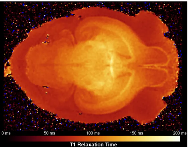
day 12 rat brain is shown in Figure 2. The average T1 relaxation time across the entire brain was approximately 110 ms.

Figure 2 - T1 relaxation time map of a stained postnatal day 12 rat brain. When soaked in a 5 mM solution of gadolinium chelate for 5-7 days, the T1 of the brain parenchyma is approximately 80-130 ms.

2.2.3. High-sensitivity RF coil design

Careful RF coil design is essential for achieving high-resolution, high-SNR images with MRH. Improper RF coil engineering can be a major source of signal loss and can cause image artifacts due to inhomogeneous coil sensitivity across the field of view. Single-loop solenoid RF coils are simple, reliable, and can produce very homogeneous RF transmit fields (Hoult and Richards, 1976). The

(35)

main reason that solenoid RF coils are not widely used is that they must be positioned perpendicular to the main magnetic field, B0, which is often impractical

for in-vivo imaging, but not for MRH. The sensitivity of a solenoid RF coil depends on a number of factors, the most important of which are surface

conductivity and internal volume (Hoult and Richards, 1976; Hoult and Lauterbur, 1979; Edelstein et al., 1986). The higher the surface conductivity the more

current (and therefore signal) is produced for a given spin excitation. Internal volume affects RF coil sensitivity in a number of ways. First, thermal noise contamination is integrated across the entire internal volume of the RF coil, so larger internal volumes will have more thermal noise and lower SNR. Second, the closer the spin excitation is to the surface of the coil the higher the resulting signal will be. Finally, the conduction path length of the solenoid is directly related to resistive losses, and shorter path lengths (i.e. smaller coils) lead to improved SNR.

For the above reasons, we attempted to make the smallest internal volume RF coils possible to accommodate the different stages of rat postnatal neurodevelopment. We also attempted to use the highest conductivity material available that would remain stable throughout the time and temperature changes that are typical for a high-resolution MRH acquisition. We chose 99.9% pure silver because of its relatively low reactivity, high conductivity, and low thermal expansion coefficient. Coils were constructed from 50 µm thick rolled silver sheets. We fabricated three different sized coils to cover the range of brain sizes included in our study, each with a different internal diameter (ID): 20 mm ID for

(36)

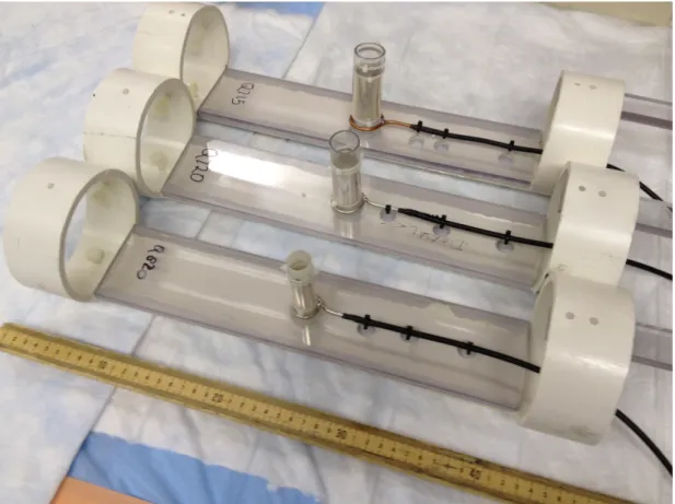
birth–postnatal day 8, 25 mm ID for postnatal day 12–24, and 30 mm ID for postnatal day 40–80. In each case, the length of the solenoid was chosen to be approximately 1.5 times the internal diameter to produce a homogeneous RF transmit field. All three RF coils are shown in Figure 3 with a ruler for scale comparison.

Figure 3 - The three RF coils designed for imaging rat postnatal neurodevelopment. From the top of the figure: 30 mm ID coil, 25 mm ID coil, 20 mm ID coil, centimeter ruler.

We quantified the sensitivity of each RF coil by measuring its Q-factor—a parameter that describes how under-damped an RF resonator is by comparing its bandwidth relative to its center frequency. In general, the higher the Q-factor, the more sensitive the RF coil and the narrower its bandwidth. In theory, image

(37)

numerically equivalent to the resonant frequency divided by the -3 dB bandwidth (Edelstein et al., 1986). A typical copper MRH coil for a 7T imaging system has a Q-factor for 400-500. The silver coils designed for this study had Q-factors of 820, 720, and 715 for the 20 mm ID, 25 mm ID, and 30 mm ID coils respectively.

2.3. Discussion

Together, the pulse sequence design, specimen preparation, and RF coil modifications described above dramatically improved SNR, and therefore

resolution, of DT-MRH experiments on the developing rat brain. With a minimum acceptable SNR threshold of 30, these modifications allow 50 µm isotropic

diffusion-weighted images a b=1492 mm2/s and 25 µm isotropic gradient recalled echo anatomic images. These represent the highest-resolution DT-MRH images of the whole rat brain ever reported. The increased spatial accuracy provided by these high-resolution images combined with the quantitative measurements of diffusion afforded by DT-MRH have extraordinary potential to reveal the complex spatiotemporal changes that occur during postnatal neurodevelopment in

unprecedented detail. Further, the approaches detailed in this chapter have widespread applicability to MRH experiments in other MRI systems, in other species, and in other organ systems with only minor modifications. For example, the rolled silver RF coil technology is already being used for mouse brain, kidney, and heart MRH in our laboratory. These improvements add to the long list of technologies that make DT-MRH both possible and practical in a large variety of model systems.

(38)

3. Acquisition of DT-MRH data throughout rat postnatal

neurodevelopment

The work presented in this chapter was published in two different articles in NeuroImage, one in 2012 (Johnson et al., 2012) and one in 2013 (Calabrese et al., 2013).

3.1. Introduction and Background

Here, we present the first MRH-based atlas of the developing rat brain. Our atlas incorporates the best features of preceding MRH-based atlases, and introduces several new features designed to increase its utility as a quantitative database for neurodevelopmental research. The atlas includes both DT-MRH and conventional anatomic MRH data at the highest spatial resolution yet reported for the whole rat brain (50 µm isotropic and 25 µm isotropic

respectively). These image voxels are 8,000-64,000 times smaller than routine clinical image voxels. The atlas comprehensively covers postnatal

neurodevelopment with nine postnatal time points chosen to accurately sample the full scope of postnatal volume changes in the rat brain. Each time point comprises data from five different specimens and includes eight distinct image contrasts, five of which are quantitative in nature. Population averages have been created for every image contrast at each time point to allow enhanced visualization and voxelwise analyses of variation.

(39)

3.2. Methods

3.2.1. Experimental animals

All experiments and procedures were done with the approval of the Duke University Institutional Animal Care and Use Committee. To ensure accurate sampling of postnatal brain growth, we selected nine time points temporally spaced to allow a fixed percentage increase in brain volume between samples based on previously published rat brain growth curves. The nine time points selected for the atlas were p0, p2, p4, p8, p12, p18, p24, p40, and p80 (where “p” indicates postnatal day). Five male, Wistar rats were selected for imaging at each time point. All animals were from litters of 10-12 pups (average = 11) and had a body weight within one standard deviation of mean weight for age based on the growth curve provided by the supplier (Charles River Wistar Rat Page, 2013).

3.2.2. Specimen preparation

Animals were perfusion-fixed using the active staining technique (Johnson et al., 2002b). Perfusion fixation was achieved using a 10% solution of Neutral Buffered Formalin (NBF) containing 10% (50 mM) Gadoteridol. After perfusion fixation, rat heads were removed and immersed in 10% NBF for 24 hours. Finally, fixed rat heads were transferred to a 0.1 M solution of Phosphate

Buffered Saline containing 1% (5 mM) Gadoteridol at 4° C for 5-7 days. Prior to imaging, specimens were placed in custom-made, MRI-compatible tubes and immersed in fomblin liquid fluorocarbon for susceptibility matching and to prevent

(40)

specimen dehydration. All imaging experiments were performed with the brain in the neurocranium to preserve tissue integrity and native spatial relationships.

3.2.3. Image acquisition

Imaging was performed on a 7 Tesla small animal MRI system (Magnex Scientific, Yarnton, Oxford, UK) equipped with 650 mT/m Resonance Research gradient coils (Resonance Research, Inc., Billerica, MA, USA), and controlled with a General Electric Signa console (GE Medical Systems, Milwaukee, WI, USA). RF transmission and reception was achieved using a series of custom solenoid coils ranging from 15 mm diameter × 30 mm long to 30 mm diameter × 50 mm long. T2*-weighted gradient recalled echo (GRE) images were acquired using a 3D sequence (TR = 50 ms, TE = 8.3 ms, NEX = 2, α=60°). The

acquisition matrix ranged from 1024 × 512 × 512 to 1600 × 800 × 800 and the field of view (FOV) ranged from 25.6 × 12.8 × 12.8 mm to 40 × 20 × 20 mm. Matrix size was chosen so that the Nyquist isotropic spatial resolution was 25 µm in all cases.

Diffusion-weighted images were acquired using a spin-echo pulse sequence (TR = 100 ms, TE = 16.2 ms, NEX = 1). Diffusion preparation was accomplished using a modified Tanner-Stejskal diffusion-encoding scheme (Stejskal and Tanner, 1965) with a pair of unipolar, half-sine diffusion gradient waveforms (width δ = 3 ms, separation Δ = 8.5 ms, gradient amplitude = 600 mT/m). One b0 image and 6 high b-value images (b=1492 s/mm2) were acquired with diffusion sensitization along each of six non-colinear diffusion gradient

(41)

vectors: [1, 1, 0], [1, 0, 1], [0, 1, 1], [-1, 1, 0], [1, 0, -1], and [0, -1, 1]. In this paper, the b0 image is referred to as “T2-weighted” because the long TR and TE of the acquisition relative to the T1 and T2 of the specimen, respectively, result in strong T2-weighting. The acquisition matrix ranged from 512 × 256 × 256 to 800 × 400 × 400 and FOV ranged from 25.6 × 12.8 × 12.8 mm to 40 × 20 × 20 mm. The Nyquist isotropic spatial resolution was 50 µm for all diffusion-weighted images. All images were derived from fully sampled k-space data with no zero-filling.

3.2.4. Diffusion tensor image processing

Diffusion data were processed with a custom image-processing pipeline comprised of freely available software packages including Perl

(http://www.perl.org), ANTs (http://www.picsl.upenn.edu/ANTS/), and Diffusion Toolkit (http://www.trackvis.org). This automated pipeline was created to ensure that all data were processed in the same way, and to reduce the potential for user error. First, diffusion-weighted image volumes were spatially normalized to the b0 volume using the ANTs rigid registration to correct for the linear portion of eddy current distortions. Next, diffusion tensor estimation, and calculation of tensor-derived data sets were performed using Diffusion Toolkit. Finally, data were organized into a consistent file architecture and archived in NIfTI format (http://nifti.nimh.nih.gov) in an on-site Oracle database (Johnson et al., 2007).

(42)

3.2.5. Image registration and averaging

Inter-specimen registration of MR data was accomplished with the ANTs software package (Avants et al., 2008; 2011). Skull-stripped (Badea et al., 2007b) GRE and DWI images from each set of specimens (5 per time point) were aligned using an affine registration, followed by an iterative, viscous fluid model, non-linear registration. We employed a Minimum Deformation Template (MDT) strategy, which uses pairwise, non-linear image registrations to construct an average template requiring the minimum amount of deformation from each of the starting points (Kochunov et al., 2001). The similarity metric used for

registration was cross-correlation computed for a kernel radius of 4 voxels. We used a multi-resolution scheme, and did a maximum of 4000 iterations at a down-sampling factor of three, 4000 iterations at a down-sampling factor of two, and 250 iterations at full resolution. We used the greedy symmetric normalization (SyN) model with a gradient step of 0.5 and a Gaussian regularization with σ = 3 for the similarity gradient, and σ = 1 for the deformation field. The algorithm converged at each step of the registration, usually with fewer than 500 iterations. The resultant transformations were applied directly to scalar images to create population averages.

3.2.6. Tensor averaging and tractography

To create population average tensor volumes we used a log-Euclidean transformation strategy (Arsigny et al., 2006). In short, the transformation is applied to the matrix logarithm of the tensor, and then the matrix exponent of the

(43)

result is taken to create the transformed tensor. FACT tractography (Mori et al., 1999) was performed on each individual and each average tensor volume using a fractional anisotropy threshold of 0.25 and an angle threshold of 45 degrees.

3.2.7. Alignment of image data to histologic atlases

We chose to align our data to conventional histology atlases for two

reasons. First, we wanted a reliable method to identify different brain regions and ensure that borders visible on MRI corresponded with true cytological borders; second, we wanted to incorporate our work in to the large body of existing neuroanatomical research on the rat brain. By doing so, we hope to facilitate intermodal research in future studies on rat neuroanatomy. MRH data were aligned towards two conventional histology atlases—the p80 data were aligned to the Paxinos and Watson adult rat atlas (Paxinos and Watson, 2007), and the p0 data were aligned to the Ashwell and Paxinos p0 rat atlas (Ashwell and Paxinos, 2008). The isotropic MR data were manually reoriented to match the coronal sectioning plans outlined in the introduction section of the two atlases. We then manually compared at least six coronal MR planes (three rostral and three caudal) with spatially unique structures near both the dorsal and ventral surfaces of the brain. Based on the observed error, we then reoriented the original MR data to more closely match the histology atlas and, once again, compared six coronal MR planes. We proceeded in this fashion until we could no longer decrease error by reorienting the MR data. MR data for time points other than p0 and p80 were automatically oriented using a rigid affine registration.

(44)

Early time point data (i.e. p2, p4, p8, and p12) were registered to the aligned p0 data, while late time point data (i.e. p18, p24, and p40) were registered to the aligned p80 data.

3.3. Results

3.3.1. Atlas orientation

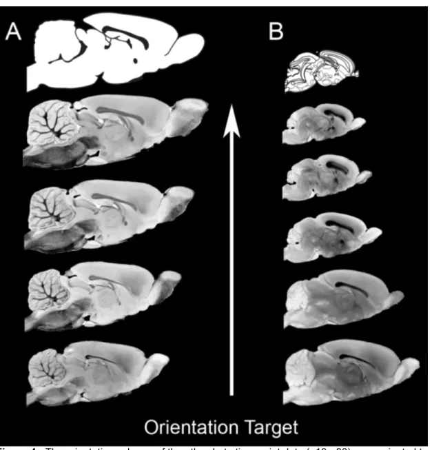
Figure 4 illustrates the orientation scheme for the atlas. Late time point data (i.e. p18 and older) were oriented to be consistent with the Paxinos and Watson adult rat atlas (column A) (Paxinos and Watson, 2007), while early time point data (i.e. p12 and younger) were oriented to be consistent with the Ashwell and Paxions neonatal rat atlas (column B) (Ashwell and Paxinos, 2008). The sectioning diagram from the respective histology atlas is included at the top of each column for reference.

(45)

Figure 4 - The orientation scheme of the atlas. Late time point data (p18-p80) were oriented to the Paxinos and Watson adult rat brain atlas (Column A). Early time point data (p0-p12) were oriented to the Ashwell and Paxinos p0 rat brain atlas. The sectioning diagrams from the respective histology atlases are shown at the top of each column.

3.3.2. Alignment of p0 image data to the Ashwell and Paxinos histology atlas

As described in the Methods section, the p0 MRH volumes were aligned to the p0 images in the Ashwell and Paxinos (2008) histology atlas using iterative manual rotation followed by comparisons of six coronal planes. An example of a coronal comparison is presented in Figure 5. In the dorsal portion of Figure 5, the

(46)

letter A marks the rostral-most crossing of the ventral hippocampal commissure (vhc), which is not present in adjacent histology sections. B denotes the posterior limb of the anterior commissure (acp), which makes its first contact with the external capsule (ec) in this section. Rostral to this plane, the acp and ec are not in contact with each other and caudally they cannot be distinguished as two separate structures. Finally, C marks the rostral-most crossing of the anterior commissure (ac), which has a distinctive oval shape across the midline that is not present in more rostral sections. The Ashwell and Paxinos atlas does not provide rostral/caudal coordinates, so we could not directly compare histologic

coordinates to MR coordinates. However, the histology sectioning interval was 200 µm, so we can compare inter-slice distance on MR and histologic sections

as a metric for alignment of the two datasets. These data are presented in Table 1. The mean discrepancy between MR coordinates and histologic coordinates was 1.06 mm, which is comparable to similar attempts at aligning MRI volumes with histology (Johnson et al., 2012).

(47)

Figure 5 - A comparison of a plate from the Ashwell and Paxinos p0 rat brain histology atlas (Ashwell and Paxinos, 2008) (left) with the oriented p0 GRE data (right). The displayed section is at the level of the caudal crossing of the anterior commissure. Letter A marks the ventral

hippocampal commissure (vhc). B marks the intersection of the posterior limb of the anterior commissure (acp) with the external capsule (ec). C marks the caudal extent of the crossing of the anterior commissure.

Table 1 - Comparison of interstice distance between corresponding coronal planes in the p0 rat brain as measured by MRI and the Ashwell and Paxinos p0 rat histology atlas (Ashwell and Paxinos, 2008) . Histology Plate #s MR Slice #s Histology Interslice Dist. (mm) MR Interslice Dist. (mm) Discrepancy (mm) 217-228 536-485 2.2 1.275 0.925 228-235 485-442 1.4 1.075 0.325 235-245 442-403 2 0.975 1.025 245-251 403-381 1.2 0.55 0.65 251-279 381-251 5.6 3.25 2.35 Mean Discrepancy (mm) 1.06

(48)

3.3.3. Alignment of p80 image data to the Paxinos and Watson histology atlas

To ensure that the adult (p80) MR data sets were oriented as closely as possible to that of the Paxinos and Watson atlas, we identified landmarks in a series of coronal slices and compared their rostrocaudal position with the same structures pictured in the Paxinos and Watson atlas. The comparisons are shown in Table 2. The mean discrepancy in 21 comparisons was 0.27 mm, which is within the range of discrepancy that exists when landmarks in the Paxinos and Watson atlas were compared in different planes. The alignment of the MRH and Paxinos and Watson atlas can be most easily appreciated in Figure 6, which shows MR slices (left) adjacent to histology slices from the Paxinos and Watson atlas (right) with relevant anatomic landmarks showing alignment accuracy.

(49)

Figure 6 - Three adjacent horizontal slices from the Paxinos and Watson atlas and the

corresponding GRE images demonstrating the alignment of MR data to histology. MR contrast has been inverted to better match histology contrast. Row A corresponds to Paxinos and Watson atlas Figure 198 (interaural 4.68). In this plane, the medial cerebellar nucleus (MedDL) is visible posteriorly, but the crossing of the posterior commissure (pc) and the genu of the corpus callosum (gcc) are not yet visible anteriorly. Row B corresponds to Paxinos and Watson Figure 199 (interaural 4.90 mm), the section immediately dorsal to Row A. The three major landmarks that define this horizontal slice are the ventralmost aspect of the gcc, the ventralmost aspect of the pc, and the dorsalmost aspect of MedDL. Row C corresponds to Paxinos and Watson Figure 200 (interaural 5.26), the section immediately dorsal to Row B. In this horizontal plane, MedDL is no longer visible, while the gcc and pc remain in plane. The corresponding MR images closely match the landmarks seen in the histology sections.

(50)

Table 2 - The rostrocaudal position of 21 landmarks in the Paxinos-Watson atlas (relative to the interaural zero) compared with their rostrocaudal position (in mm) in the MR coronal slices. In the far-right column, the discrepancy is listed in each case. The mean discrepancy was 0.27 mm.

Structure AP atlas

coordinate Slice number

Slice AP coordinate Discrepancy emergence of 7n -1.08 548 -1.075 0.005 rostral AmbC -3.00 467 -3.20 0.20 caudal IOPr -4.56 407 -4.70 0.14 caudal IOM -6.00 343 -6.30 0.30 rostral pyr decussation -5.65 332 -6.50 0.85 xscp caudal 1.08 634 0.975 0.03 4N center 1.68 657 1.55 0.13 RMC caudal 2.40 689 2.35 0.05 rcc caudal 3.72 738 3.57 0.15 fr ventral end 3.84 740 3.65 0.19 caudal mam. bodies 3.60 741 3.65 0.05 fr emerges Hb 5.40 802 5.18 0.02 caudal VMH 5.65 829 5.90 0.35 hippocampus rostral end 7.28 866 6.77 0.61 sox middle 7.56 916 8.05 0.41 rostral LOT 8.28 892 7.50 0.78 rostral to ac 9.00 955 9.00 0.00 rostral end of CPu 11.76 1050 11.37 0.39 ventral taenia tecta - middle 13.20 1125 13.25 0.05 frontal pole 15.12 1171 14.4 0.72 caudal GlA 14.64 1160 14.1 0.54

(51)

3.3.4. Atlas dimensionality

The final atlas is truly multidimensional, being comprised of the three spatial dimensions, the fourth dimension of time (neurodevelopment) and a fifth dimension of image contrast. Figure 7 attempts to capture the high level of dimensionality of the atlas. On the left side of the figure, T2-weighted horizontal slices through the genu of the corpus callosum are shown for each of the nine atlas time points, increasing from postnatal day zero (p0) at the top to postnatal day 80 (p80) at the bottom. Figure 7A shows a three-plane view of the p0

gradient recalled echo volume, illustrating that each time point features isotropic data comprising the three spatial dimensions of the atlas. Figure 7B displays the average whole-brain tractography set from the p18 time point. Tractography segments are colored based on orientation of the primary eigenvector following standard coloring convention (red= left/right; green = rostral/caudal; blue = dorsal/ventral). Each atlas time point has five individual tractography volumes and a sixth, average tractography volume derived from the average tensor. Figure 7C demonstrates the MR contrast dimension of the atlas by displaying the seven other image contrasts (excluding T2-weighted) that exist for each time point. The abbreviations used for the different contrasts are listed in Table 3.