Estimation via L1-Norm Regularization
.
White Rose Research Online URL for this paper:
http://eprints.whiterose.ac.uk/125541/
Article:
Shi, Q., Lu, H. and Cheung, Y.M. (2017) Rank-One Matrix Completion with Automatic Rank
Estimation via L1-Norm Regularization. IEEE Transactions on Neural Networks and
Learning Systems. ISSN 2162-237X
https://doi.org/10.1109/TNNLS.2017.2766160
promoting access to
White Rose research papers
[email protected] http://eprints.whiterose.ac.uk/Rank-One Matrix Completion with Automatic Rank
Estimation via L1-Norm Regularization
Qiquan Shi,
Student Member, IEEE,
Haiping Lu,
Member, IEEE
, and Yiu-ming Cheung,
Senior Member, IEEE
Abstract—Completing a matrix from a small subset of its
entries, i.e., matrix completion, is a challenging problem arising from many real-world applications, such as machine learning and computer vision. One popular approach to solving the matrix completion problem is based on low-rank decomposi-tion/factorization. Low-rank matrix decomposition-based meth-ods often require a pre-specified rank, which is difficult to determine in practice. In this paper, we propose a novel low-rank decomposition-based matrix completion method with automatic
rank estimation. Our method is based on rank-one approximation
where a matrix is represented as a weighted summation of a set of rank-one matrices. To automatically determine the rank of an incomplete matrix, we impose L1-norm regularization on the weight vector and simultaneously minimize the reconstruction error. After obtaining the rank, we further remove the L1-norm regularizer and refine recovery results. With a correctly estimated rank, we can obtain the optimal solution under certain conditions. Experimental results on both synthetic and real-world data demonstrate that the proposed method not only has good performance in rank estimation, but also achieves better recovery accuracy than competing methods.
Index Terms—Rank estimation, matrix completion, rank-one
approximation, low-rank decomposition.
I. INTRODUCTION
Matrix completion aims to recover a whole matrix from its partial observations. It has witnessed a burst of activities, motivated by many applications such as machine learning [1]– [5], image processing [6]–[8], and computer vision [9]–[11]. Most existing methods assume the target matrix has a low-rank structure since most real-world data (e.g., images) are low-rank or approximately low-rank. Thus, for a target matrix
M ∈ RI1×I2 with partial observations in an index set Ω,
the matrix completion problem can be formulated as a rank minimization problem:
min
X rank(
X) s.t. PΩ(X) =PΩ(M), (1)
whererank(X)is the rank of X∈RI1×I2, andΩ∈RI1×I2
is the binary index matrix: Ωij = 1 if Xij is observed, and
Ωij = 0 otherwise. PΩ is the associated sampling operator
which acquires only the entries indexed by Ω. However, the
model (1) is NP-hard due to the non-convexity and
combina-tional nature of therank function.
To address this problem, a popular convex relaxation of rank function is based on minimization of the nuclear norm (a.k.a.,
Qiquan Shi and Yiu-ming Cheung are with the Department of Com-puter Science, Hong Kong Baptist University, Hong Kong (e-mail: [email protected] and [email protected]). Yiu-ming Cheung is the corresponding author. Haiping Lu is with the Department of Computer Science, University of Sheffield, U.K. (e-mail: [email protected]).
trace norm or Schattenp-norm withp= 1) [1], [12]–[14]. In
this way, the rank minimization model (1) is rewritten as a nuclear norm minimization model:
min
X k
Xk∗ s.t. PΩ(X) =PΩ(M), (2)
where the nuclear normkXk∗is the summation of the singular
values of X. Assuming the observed entries are uniformly
sampled from the original matrix M, Cand`es and Recht [1]
prove that the missing entries can be exactly recovered ifM
(with rankR) satisfies certain incoherence conditions and
ob-serves at leastO(N1.2Rlog(N)) (N = max(I
1, I2)) entries.
This sampling bound is narrowed to O(N Rlog(N))in [13].
A number of nuclear norm minimization-based algorithms have been proposed to solve the convex model (2). Singu-lar Value Thresholding (SVT) [15] employs the linearized Bremgan iterations [16] to solve the dual of a regularized approximation of (2). Accelerated Proximal Gradient with Linesearch algorithm (APGL) [17] accelerates the convergence of SVT by a fast iterative shrinkage thresholding algorithm [18]. Fixed Point Continuation with Approximate singular value decomposition (SVD) (FPCA) [19] addresses the same problem as APGL while utilizing a fast Monte Carlo algorithm for SVD calculations. Soft-Impute [20] exploits a “sparse plus low-rank” structure to allow efficient SVD in each iteration, with accelerated version (AIS-Impute) in [21]. Other well-known works include [22]–[26].
Another class of techniques is based on low-rank matrix decomposition/factorization, which is more suitable for
large-scale cases. Since any matrixZ∈RI1×I2 can be modeled in
a bilateral factorization form:UV⊤, whereU∈RI1×R,V∈
RI2×R, the low-rank decomposition-based matrix completion
model is formulated as:
min
Z,U,V k
Z−UV⊤k2
F s.t. PΩ(Z) =PΩ(M), (3)
where the integerR (R <min(I1, I2))is the rank of matrix
M. Gradient-based optimization algorithms such as alternating
minimization methods [27]–[30] are widely used to solve the model (3). Although (3) is non-convex, many works demon-strate that low-rank decomposition-based methods can perform more efficiently and are empirically as reliable as the convex methods [31]–[38]. Besides, there have been some works [27], [38], [39] that provide theoretical guarantee for their
performance. For example, Jainet al.[27] theoretically prove
that the alternating minimization also can exactly recover the matrix under certain conditions similar to the conditions given in [1] (decomposition-based methods may require more observations than nuclear norm minimization-based methods
Many matrix completion methods especially low-rank matrix decomposition-based methods often require a pre-specified rank. Determining the rank of an incomplete matrix is a challenging task, with several existing studies [35], [40]–
[44]. Based on the model (3), Wen et al. [35] propose a
low-rank matrix fitting algorithm (LMaFit) that estimates the rank by two heuristic strategies (decreasing rank strategy and increasing rank strategy) and solve it by a nonlinear
successive over-relaxation method [45]. Keshavan et al.[39],
[40], [46] reformulate the LMaFit model (3) into an SVD form and propose a gradient descent algorithm on Grassmann manifold (OptSpace), which integrates the spectral techniques with manifold optimization and determines the rank by com-puting the SVD of the trimmed observations [40]. Recently, MaCBetH [43] is proposed to improve OptSpace by a different spectral procedure that detects the rank (by estimating the negative eigenvalues of a Bethe Hessian matrix) and a better initialization for the approximation minimization. These three methods have achieved good performance of rank estimation on synthetic matrices while they do not work well on real-world images, at least in our preliminary studies. On the other hand, for a fixed-rank smooth Riemannian manifold algo-rithm named LRGeomCG [47], Uschmajew and Vandereycken propose GeomPursuit [44] that adds a greedy outer iteration
to LRGeomCG to increase the rank with a step-size l for
better recovery performance. Based on our empirical studies, however, GeomPursuit does not obtain exact true ranks and becomes much slower for larger matrices.
Rank-one approximation is a specific low-rank matrix decomposition popularly used in matrix completion [48]–
[53]. Here, any matrix Z is represented as the weighted
summation of R factorized rank-one matrices: Z =
PR
r=1wrurv⊤r = Udiag(w)V⊤, where the weight vector
w = [w1,· · ·, wr,· · ·, wR]⊤,U ∈ RI1×R ={u
r}Rr=1,V ∈ RI2×R ={v
r}Rr=1. Actually, SVD is a special rank-one
ap-proximation whose factors{ur}R
r=1and{vr}Rr=1are
orthogo-nal, and it is used in OptSpace. Wanget al.[50], [51] recently
propose an efficient rank-one matrix pursuit method (R1MP) by extending orthogonal matching pursuit to the matrix case. R1MP usually achieves better results given a rank higher than the true rank. In other words, R1MP cannot estimate the rank and does not pursue a low-rank approximation.
In this paper, we propose a novel rank-one matrix
completion method with automatic rank estimation. Under
the low-rank assumption, we aim to automatically determine the rank of an incomplete matrix and recover the matrix. When a rank is given, we can minimize the reconstruction error of the rank-one approximation via least squares to
predict the missing entries. We present it asRank-One Matrix
Completion (R1MC). With a correctly estimated rank, R1MC
likes other fixed-rank methods such as [32], [47], [54] can achieve the optimal solution for matrix completion under certain conditions [1], [27], according to the Eckart–Young– Mirsky theorem [55], [56]. However, the rank estimation is a difficult task for incomplete matrices. By solving this problem, the main contributions of this paper are:
• We address the rank estimation problem by imposing an
L1-norm regularization on the weight vector (analogous
to the vector of singular values) while minimizing the
reconstruction error. We call this L1-norm regularized
rank-oneMatrixCompletion method with automatic rank
estimationas L1MC.
• We further develop L1MC with refinement (L1MC-RF)
by proposing a refinement strategy: once the rank
is automatically determined by L1MC, we remove the L1-norm regularization, and further refine the recovery results by directly minimizing the reconstruction errors via R1MC. Essentially, L1MC-RF integrates L1MC and R1MC, while R1MC can be replaced by other fixed-rank completion methods such as [32].
Thus, L1MC-RF can automatically estimate the true rank and exactly predict the missing entries under certain conditions [1], [32], [57]. We solve the optimization problem by the block coordinate descent approach (a.k.a., alternating minimization method or nonlinear (block) Gauss-Seidel scheme), where each variable is iteratively updated with all the others fixed.
In the next section, we review necessary preliminaries and related works. We present the proposed methods in Sec. III and then evaluate them in Sec. IV. Finally, a conclusion is drawn in Sec.V.
II. PRELIMINARIES ANDRELATEDWORKS
A. Notations
In this paper, a vector is denoted by a bold lower-case
letter x ∈ RI and a matrix is denoted by a bold capital
letter X ∈ RI1×I2. The ith entry of a vector a ∈ RI is
denoted byai, and the(i, j)th entry of a matrixXis denoted
by Xij. The Frobenius norm of a matrix X is defined by
kXkF = phX,Xi. Ω ∈ RI1×I2 is a binary index matrix:
Ωij = 1ifXij is observed, andΩij = 0otherwise.PΩis the
associated sampling operator which acquires only the entries
indexed byΩ, defined as:
(PΩ(X))ij =
(
Xij, if(i, j)∈Ω
0, if(i, j)∈Ωc , (4)
where Ωc is the complement of Ω. We have PΩ(X) +
PΩc(X) =X.
B. The Eckart–Young–Mirsky Theorem
Given a matrix M ∈ RI1×I2 with rank R (with singular
values of M {σ1 ≥ · · ·σp ≥ σp+1 ≥ · · · ≥ σR > 0}),
the optimal low-rank approximation is given by a truncated
SVD of M according to the classical Eckart–Young–Mirsky
theorem [55], [56]. That is, if M = UΣV⊤, then Mp =
Pp
i=1σi uiv⊤i is the unique optimal rank-p approximation
(p < R)ofM. We present the Eckart–Young–Mirsky theorem
under Frobenius norm in Theorem 1 following [58]. This
theorem is employed for matrix/tensor decompositions in [12], [58], [59].
Theorem 1. (The Eckart–Young–Mirsky Theorem) Let
M ∈ RI1×I2 has rank R < min(I
1, I2) and its
SVD is: M = UΣV⊤ = PR
i=1σiuiv⊤i , where Σ =
diag(σ1,· · · , σp,· · · , σR,0,· · · ,0) and σ1 ≥ · · ·σp ≥
matrices with rankp < R <min(I1, I2). The unique optimal
solution of:
min
A∈Mk
M−Ak2F, s.t. rank(A) =p (5)
is given by the rank-papproximation (truncated SVD) of M:
Mp=Pp i=1σiuiv⊤i , and we have min A∈M k M−Ak2 F =kM−Mpk2F = R X j=p+1 σj2 (6)
C. Existing Completion Methods with Rank Estimation Rank estimation is important for matrix completion meth-ods requiring a rank a priori [36], [60]. The state-of-the-art matrix completion methods with automatic rank estimation are LMaFit [35], Optspace [39], [40], [46], MaCBetH [43], and GeomPursuit [44].
LMaFit: Based on the low-rank matrix decomposition
model (3): minZ,U,VkZ−UV⊤k2F s.t.PΩ(Z) = PΩ(M),
LMaFit [35] is proposed to heuristically estimate a rank starting from an over-estimated rank or under-estimated rank (initially higher or lower than the true rank) for matrix completion. Moreover, LMaFit only requires solving a linear least squares problem per iteration instead of a SVD and integrates an efficient nonlinear successive over-relaxation scheme to accelerate the convergence.
OptSpace: Keshavan et al. [46] propose OptSpace with another matrix decomposition form (SVD form):
min
U,Σ,V k
X−UΣV⊤k2
F s.t. PΩ(X) =PΩ(M), (7)
where the factor matrices UandVhave orthogonal columns
andΣ is a diagonal matrix. OptSpace consists of three steps
[40], [46]. First, it trims the observed matrix PΩ(M) by
setting to zero all rows (resp. columns) with more observed entries than twice the average number of observed entries per
row (resp. per column). Second, it computes the best rank-R
approximation of the trimmed matrix via sparse SVD, where
the rank R is estimated as the singular value index if the
ratio between two consecutive singular values is minimum [40]. Third, it minimizes the reconstruction error via a special gradient descent method over the Grassmann manifold. Be-sides, the authors further provide the performance guarantee for OptSpace under moderate incoherence condition [39].
MaCBetH: Recently, Alaa et al. [43] propose MaCBetH to improve OptSpace by replacing the first two steps with a different spectral procedure that detects a rank and provides a better initialization for the approximation minimization. In MaCBetH, the rank is estimated as the number of negative eigenvalues of the Bethe Hessian matrix, and the correspond-ing eigenvectors are used as initial conditions for minimizcorrespond-ing the difference between the predicted matrix and the observed entries [43].
GeomPursuit: Another state-of-the-art algorithm,
Geom-Pursuit [44], combines a greedy outer iterationthat increases
the rank with a step-sizelwitha smooth Riemannian algorithm
LRGeomCG [47] that optimizes the cost function on a
fixed-rank manifold. In other words, LRGeomCG needs a fixed rank as input while GeomPursuit can estimate the rank via
Greedy rank updates. Based on the empirical studies, however, we found that GeomPursuit cannot obtain exact true ranks though it improves the recovery performance of LRGeomCG.
Moreover, it is sensitive to the step-sizel and becomes much
slower for larger matrices.
On the other hand, FBCP [61] is one of recent tensor
completion methods which can automatically determine the rank of an incomplete tensor (a matrix is a second-order ten-sor), where the authors formulate CANDECOMP/PARAFAC (CP) decomposition [62], [63] using a hierarchical probabilis-tic model and employ a fully Bayesian treatment for automaprobabilis-tic rank estimation. Our rank-one approximation model (10) (to be presented in Section III) can be considered as the matrix case of CP decomposition. Here we degenerate FBCP to matrix case to compare with ours and other existing methods. D. Existing Rank-One Matrix Completion Methods
Given a matrix Z ∈ RI1×I2, it can be written as a linear
combination of rank-one matrices by extending the atom decomposition [64] to matrix case [48], [50], [52]:
Z=Y(θ) =X
i∈I
θiYi, (8)
where {Yi, i ∈ I} is the set of rank-one matrices
with kYikF = 1, and θ is the weight vector: θ =
[θ1,· · · , θi,· · · , θ|I|]⊤. Here, the weight vector θ includes infinite number of weights [50].
Based on the model (8), Wanget al.[50], [51] reformulate
the matrix completion problem as (9), and propose rank-one matrix pursuit (R1MP):
min
θ kP
Ω(Y(θ)−M)k2F s.t. kθk0≤c, (9)
where c is an integer and kθk0 denotes the cardinality of
the number of nonzero elements of θ. R1MP alternatively
constructs rank-one basis matrices and learns weights of the bases by orthogonal matching pursuit method. R1MP can efficiently obtain better results given a rank higher than the true rank of the original (complete) matrix. In other words, R1MP cannot automatically estimate the rank of an incomplete matrix and does not pursue a low-rank approximation.
III. PROPOSEDMETHODS
We can represent any matrixZ ∈RI1×I2 as the weighted
summation ofR factorized rank-one matrices:
Z = R X r=1 wrurv⊤r = Udiag(w)V⊤ s.t.kurk2=kvrk2= 1, forr= 1,· · ·, R, (10)
where the weight vector w = [w1,· · ·, wr,· · ·, wR]⊤,U ∈
RI1×R = {u
r}Rr=1,V ∈ RI2×R = {vr}Rr=1, and R (R <
min(I1, I2))is the rank ofZ.
Remark 1: This model (10) is different from the model (8) used in [50], [52]: the number of weights (analogous to singular values) of (10) is finite and should be small (low-rank), and we represent each rank-one matrix in a factorization form. Besides, our model (10) is similar to the SVD form (used
Vof our model are not enforced to be orthogonal. In addition, our rank-one matrix decomposition can also be considered as the matrix case of CP decomposition.
Next, we present R1MC and develop our methods L1MC and L1MC-RF progressively.
A. Rank-One Matrix Completion (R1MC) Given True Rank Based on the rank-one approximation model (10), given a
low-rank matrix M∈RI1×I2 with partially observed entries
in Ω, i.e., PΩ(M), we reformulate the matrix completion
problem as: min X,Z 1 2kX−Zk 2 F s.t. Z= R X r=1 wrurv⊤r,PΩ(X) =PΩ(M), kurk2=kvrk2=1, for r= 1,· · · , R, (11)
whereZ is the summation of Rrank-one matrices. Here, we
assume the true rank R is known, and we can minimize the
reconstruction error via least squares to predict the missing
entries. We summarize this Rank-One Matrix Completion
method (R1MC) inAlgorithm1.
Remark 2: R1MC shares the same spirit as Iterative Hard Thresholding (IHT) [54], [65] and Singular Value Projection (SVP) [32], where the SVD of the target matrix is truncated
by keeping the topR singular values and associated singular
vectors. On the other hand, R1MC requires less parameter tuning, e.g., no step-size parameter required in [32], [54],
[65], so it is simpler to implement and use.Differentfrom the
convex completion methods such as [1] which relax the rank function via nuclear norm using soft singular value thresh-olding, R1MC is a non-convex method and obtains a
low-rank solution using hard singular value thresholding. Unlike
the methods in [27] which optimize the underlying matrix in a bilateral factorization form, the matrix is represented as a set of rank-one matrices in R1MC.
Remark 3: If M (with rank R) obeys the incoherence property and observes enough randomly sampled entries [1], R1MC can exactly recover the missing entries with high probability. The theoretical guarantees of IHT (R1MC) is first conjectured in [32], and recently [57] theoretically improves the sampling bound for IHT (R1MC): R1MC converges to the exact low-rank solution when the number of known entries is
more thanO(N R2log2
(N)), N= max (I1, I2). Furthermore,
Weiet al.[57] demonstrate that this sampling complexity can
achieve the optimal one O(N R) empirically. In other words,
for an incomplete matrixXwith enough observed entries from
M(i.e.,PΩ(X) =PΩ(M)), the missing entries of Mcan be
exactly recovered. In R1MC, we predict the missing entries by
iteratively updating: PΩc(X) = PΩc(Z) and computing the
rank-R approximation ofXby the truncated SVD ofX, and
finally recover the matrix exactly under the above assumptions.
On the other hand, the unique optimal rank-R approximation
of M is given by the truncated SVD of M according to the
Eckart–Young–Mirsky theorem (Theorem 1).
In this way, assuming the true rank R is known, R1MC
can achieve the optimal solution for matrix completion under
Algorithm 1 Rank-One Matrix Completion (R1MC)
1: Input:Incomplete matrixPΩ(M), index matrixΩ, given
rank R, maximum iterations K, and stopping tolerance
tol.
2: Initialization: PΩ(X) = PΩ(M), PΩc(X) = 0, Z =
zeros(I1, I2).
3: fork= 1, ..., K do
4: Compute the rank-Rapproximation ofX:[U0Σ0V0]=
svd(X),U0 ={ur}R
r=1 ∈RI1×R,Σ0∈RR×R,V0 =
{vr}R
r=1∈RI2×R.
5: Set Z=U0Σ0V⊤0.
6: Update the missing entries by:PΩc(X) =PΩc(Z).
7: If kPΩ(X− Z)kF/kPΩ(X)kF < tol or kXk+1 −
Xkk
F/kXk+1kF <tol, break; otherwise, continue.
8: end for
9: output: Z.
the appropriate conditions. If the input rank is higher (over-estimate) or lower (under-(over-estimate) than the true rank, it may result in poor recovery performance. Therefore, it is important to determine a good rank value (true rank) for low-rank matrix decomposition for matrix completion [36].
B. L1-norm Regularized Rank-One Matrix Completion with Automatic Rank Estimation (L1MC)
To address the important rank estimation issue, we impose
L1-norm regularization on the weight vector w and
reformu-late the R1MC model (11) as follows:
min X,w,{ur,vr}Rr=1,R µkwk1+1 2kX− R X r=1 wr urv⊤rk2F, s.t. PΩ(X) =PΩ(M), kurk2=kvrk2= 1, forr= 1,· · · , R, (12)
whereµ is the regularization parameter and R is the rank to
be estimated. By simultaneously minimizing the L1-norm reg-ularization and the reconstruction error, we can automatically determine the rank of an incomplete matrix and simultaneously
predict the missing entries. We name this new L1-norm
reg-ularized rank-oneMatrix Completion method with automatic
rank estimation asL1MC.
Remark 4:Note that the weightsin model (11) are
analo-gous to thesingular values. L1-norm regularization makes the
weight vector sparse and leads to a low-rank solution. Derivation of L1MC via BCD: we employ the Block Coordinate Descent (BCD) method [66] for optimiza-tion. The BCD method is also known as the alternat-ing minimization method or nonlinear (block) Gauss-Seidel
scheme. We divide the target variables into R+ 1 blocks:
{{w1,u1,v1},· · ·,{wr,ur,vr},· · ·,{wR,uR,vR},X}. We optimize a group (block) of variables while fixing the other groups (blocks), and update one variable while fixing the other variables in each group. After finishing the update of these
R+ 1blocks variables, we finally determine the rank.
The Lagrangian function with respect to the r-th block
Lwr,urvr = µ|wr|+ 1 2kXr−wrurv ⊤ rk 2 F, s.t.Xr=X− r−1 X q=1 wquqv⊤q, PΩ(X) =PΩ(M),kurk2=kvrk2= 1, (13)
whereXr is the residual of the approximation.
1) Updateur,vr: The function (13) with respect touris,
Lur = 1
2kXr−wrurv
⊤
rk2F (14)
Then we set the partial derivative of Lur with respect to ur
to zero, and get:
w2rur−wrXrvr= 0⇒ur(k+1)=X k rvkr wk r . (15) We normalize u(rk+1)= u (k+1) r
ku(rk+1)k2. Note that we only update
the blocks with non-zero weights (e.g., wk
r 6= 0).
Similarly, we can update vr(k+1)by,
vr(k+1)=X ⊤ r k ur(k+1) wk r , (16) and normalizevr(k+1)= v (k+1) r kvr(k+1)k2.
2) Update wr : The function (13) with respect towr is,
Lwr =µ|wr|+ 1
2kXr−wrurv
⊤
rk2F. (17)
Then we set the partial derivative of Lwr with respect towr
to zero, ∂Lwr ∂wr =µ|wr| ∂wr + wr−trace(vru⊤rXr) =µ|wr| ∂wr + wr− hXr,vru⊤ri= 0. (18)
According to Eq. (18), we know wr=hXr,vru⊤ri −µ
|wr|
∂wr.
Based on the soft thresholding algorithm [67] for L1-norm
regularization, we update w(rk+1) by:
w(rk+1)=shrinkµ(hXkr, vr(k+1)u⊤r
(k+1)
i), (19)
whereshrink is the soft thresholding operator [18], [67]:
shrinkµ(a) = a−µ (a > µ) 0 (|a| ≤µ) a+µ (a <−µ) . (20)
3) Update X: The function (12) with respect toXis,
min X 1 2kX− R X r=1 wrurv⊤rk2F, (21) s.t. PΩ(X) =PΩ(M), kurk2=kvrk2= 1.
By deriving simply the Karush-Kuhn-Tucker (KKT)
con-ditions for Eq. (21) [68], we can update X(k+1) by
X(k+1) = PΩ(X) + PΩc(Z(k+1)), where Z(k+1) = PR r=1w (k+1) r u(rk+1)v⊤r (k+1) .
Algorithm 2 L1-norm Regularized Rank-One Matrix
Completion with Automatic Rank Estimation (L1MC)
1: Input:Incomplete matrixPΩ(M), index matrixΩ,
regu-larization parameterµ, initial rankRˆ, maximum iterations
K, and stopping tolerance tol.
2: Initialization:Initialize{w={wr}Rˆ
r=1,{ur∈RI1,vr∈
RI2,ku
rk2 = kvrk2 = 1}Rrˆ=1} randomly (normal
dis-tribution); Set Z = zeros(I1, I2), PΩ(X) = PΩ(M),
PΩc(X) =0.
3: fork= 1, ..., K do
4: Xr = X.
5: forr= 1, ...,Rˆ do
6: if wr6= 0 then
7: Update ur andvr by (15) and (16) respectively.
8: Update wr by (19).
9: Xr=Xr−wrurv⊤r.
10: end if
11: end for
12: UpdateX:UpdateZ=X−Xrand the missing entries
by: PΩc(X) =PΩc(Z).
13: If kPΩ(X− Z)kF/kPΩ(X)kF < tol or kXk+1 −
Xkk
F/kXk+1kF <tol, break; otherwise, continue.
14: end for
15: Rank Estimation: Only keep the wr if wr>(10−3×
SamplingRatio×sum(w)), and then R∗ = length(w),
and keep corresponding{ur}R∗
r=1 and{vr}R
∗
r=1.
16: output: R∗,Z.
4) Estimate the Rank R : After iteratively updating all
the above variables till convergence or reaching the maximum iterations, we finally determine a rank. By checking the weight
vectorw, we only keep the weights larger than a threshold (we
set the threshold at10−3×Sampling Ratio×T otalW eight),
i.e., removing the zero and small weights which account for a very small proportion of total weights. Finally, the number
of the remaining weights in w is the estimated rank and we
keep the corresponding factors.
We summarize this new matrix completion method with
automatic rank estimation, L1MC, in Algorithm 2. In
ad-dition, since we need a initial rank for optimizing our L1MC
objective function (12), we denote Rˆ as the initial rank for
rank estimation.
Remark 5: In L1MC, we set the threshold in rank
estimation at 10−3 ×SamplingRatio×T otalW eight, i.e.,
removing small weights (analogous to singular values) less
than 0.01% to 0.09% of total weights for data with SR =
10%−90%observed entries, respectively. This setting follows
the similar idea in [69], where the low-rank matrix is truncated
by removing small singular values less than 1% of the
L2-norm of the vector of singular values. Furthermore, based on empirical studies, this threshold can be loose to be an ideal value 0 on the synthetic matrices (and real data with
SR > 30%). By only removing small singular values which
account for a very small proportion of total singular values, we keep most information of the target matrix. This threshold for rank estimation can be fixed with no need of tuning. It
works well in all tested synthetic and real data although we do not have theoretical guarantee for it yet.
Algorithm 3 L1MC withRefinement (L1MC-RF)
1: Input:Incomplete matrixPΩ(M), index matrixΩ,
regu-larization parameterµ, initial rankRˆ, maximum iterations
K, and stopping tolerancetol.
2: Step 1:ObtainR∗ byAlgorithm 2L1MC.
3: Step 2: Feed the estimated rank R∗ into Algorithm 1
R1MCto further optimize factors and weights.
4: output:R∗,Z.
C. L1MC with Refinement (L1MC-RF)
L1MC can automatically estimate the rank and simulta-neously predict the missing entries. However, the L1-norm regularization of model (12) restricts L1MC to directly opti-mize the factors and weights of rank-one approximation. To
improve the recovery performance, we propose arefinement
strategy. We refine the recovery results by directly minimizing
the reconstruction error without the L1-norm regularization
after rank estimation, i.e., we firstly determine the rank of an
incomplete matrix by L1MC, and then we remove the
L1-norm regularizer and further improve the recovery accuracy. Thus, after the rank estimation step, we reformulate the L1MC model (12) as: min X,{ur,wr,vr}R ∗ r=1 1 2kX− R∗ X r=1 wr urv⊤rk2F, s.t. PΩ(X) =PΩ(M), kurk2=kvrk2= 1, for r= 1,· · · , R∗. (22)
The formulation (22) is equivalent to the R1MC model (11). Therefore, we can directly optimize the factors and weights by R1MC to further refine the recovery results. Note that we also can further refine the recovery results of L1MC by other fixed-rank completion methods such as SVP [32], IHT [54], [65], LRGeomCG [47] and so forth, while R1MC is simpler to implement and use. We denote this integrated-solution as
L1MC with Refinement, i.e., L1MC-RF, summarized in
Algorithm 3.
In the following section, we evaluate the rank estimation and recovery accuracy of the proposed methods on the synthetic matrices and real-world images.
IV. EXPERIMENTALRESULTS
We evaluate the performance of the proposed methods from three aspects: i) parameter sensitivity and convergence; ii) importance of estimating the true rank; iii) accuracy of recovery and rank estimation over various sampling ratios
given incomplete matrices. We sample10%−90%entries from
each matrix uniformly at random for training and use “SR”
for this Sampling Ratio (training ratio). We implemented our
methods in MATLAB and all experiments were performed on a PC (Intel Xeon(R) 3.40GHz, 64GB memory).
(a) Original Lenna image.
Rank (Lenna image)
20 40 60 80 100 120 140 160 180 200 Singular Value ×104 0 1 2 3 4 5 6 7
(b) First 200 singular values of Lenna. Figure 1. An example of low-rank image.
A. Experimental Settings
1) Data: Following [17], [19], [35], [43], we generate
the synthetic matrices: M ∈ RI1×I2 with rank R from
two random matrices M1 ∈ RI1×R and M
2 ∈ RI2×R
with i.i.d. standard Gaussian entries, i.e., M = M1M⊤2. In
this paper, we report the results of five synthetic matrices:
{500×500 (R= 5),1000×1000 (R= 25),1000×1000 (R= 50),2000×2000 (R= 50),2000×2000 (R= 100)}.
Moreover, the minimum sampling ratios for guaranteeing
the exact recovery of these five matrices are (O(N R(I1×log(I2)N))):
{O(6.21%), O(17.27%), O(34.54%), O(19%), O(38%)} re-spectively using nuclear norm minimization-based methods according to [13] (decomposition-based methods may need more observations [27]).
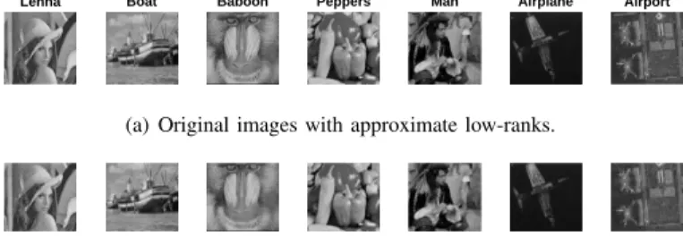
Lenna Boat Baboon Peppers Man Airplane Airport
(a) Original images with approximate low-ranks.
(b) Truncated images with exact low-ranks. Figure 2. Seven real images used for experiments.
Real data1:
We also evaluate our methods on seven
real-world images:{Lenna (512×512), Boat (512×512), Baboon
(512 × 512), Peppers (512 × 512), Man (1024 × 1024),
Airplane (1024 × 1024), Airport (1024 × 1024)}. These
natural images are approximately low-rank by observing their singular values, as shown in Fig. 1. Following [35] where the authors truncated the SVD of the Boat image to obtain the rank-40 image, we examined the singular value of these images and truncated their SVD to get the images
with exact low-ranks: {29 (Lenna), 40 (Boat), 24 (Baboon),
30 (Peppers), 27 (Man), 23 (Airplane), 22 (Airport)}, as
shown in Fig. 2. Similarly, the minimum sampling ratios for guaranteeing the exact recovery of these low-rank images are:
{O(35.33%), O(48.74%), O(29.24%), O(36.55%), O(18.28%),
O(15.57%), O(14.89%)} respectively using nuclear norm
minimization-based methods.
1Boat image is from http://lmafit.blogs.rice.edu/ and other images are available at http://sipi.usc.edu/database/database.php?volume=misc&image.
5 10 15 20 25 30 35 40 45 50 55 60 65 70 75 80 85 90 95100 Vaule of µ (500 × 500, R=5) 0 5 10 15 Estimated Rank SR=10% SR=20% SR=30% SR=40% SR=50% SR=60% SR=70% SR=80% SR=90% (a)500×500 (R= 5) 5 2035 5065 8095 110 125 140 155 170 185 200 Vaule of µ (1000 × 1000, R=50) 0 25 50 75 100 125 Estimated Rank SR=10% SR=20% SR=30% SR=40% SR=50% SR=60% SR=70% SR=80% SR=90% (b)1000×1000 (R= 50) 5 10 15 20 25 30 35 40 45 50 55 60 65 70 75 80 85 90 95100 Vaule of µ (500 × 500, R=5) 10-15 10-10 10-5 100 RSE SR=10% SR=20% SR=30% SR=40% SR=50% SR=60% SR=70% SR=80% SR=90% (c)500×500 (R= 5) 520 35 50 65 80 95 110 125 140 155 170 185 200 Vaule of µ (1000 × 1000, R=50) 10-15 10-10 10-5 100 RSE SR=10% SR=20% SR=30% SR=40% SR=50% SR=60% SR=70% SR=80% SR=90% (d)1000×1000 (R= 50)
Figure 3. Estimated ranksandRSEof recovering two synthetic matrices via L1MC-RF with (a) (c):µ∈[5 : 5 : 100] and (b) (d):µ∈[5 : 5 : 200], respectively. 5 25 45 65 85105 125 145 165 185 205 225 245 Initial Rank (500×500, R=5) 0 5 10 15 Estimated Rank SR=10% SR=20% SR=30% SR=40% SR=50% SR=60% SR=70% SR=80% SR=90% (a)500×500 (R= 5) 105090 130 170 210 250 290 330 370 410 450 490 Initial Rank (1000×1000, R=50) 0 25 50 75 100 125 Estimated Rank SR=10% SR=20% SR=30% SR=40% SR=50% SR=60% SR=70% SR=80% SR=90% (b)1000×1000 (R= 50) 5 25456585 105 125 145 165 185 205 225 245 Initial Rank (500×500, R=5) 10-15 10-10 10-5 100 RSE SR=10% SR=20% SR=30% SR=40% SR=50% SR=60% SR=70% SR=80% SR=90% (c)500×500 (R= 5) 105090 130 170 210 250 290 330 370 410 450 490 Initial Rank (1000×1000, R=50) 10-15 10-10 10-5 100 RSE SR=10% SR=20% SR=30% SR=40% SR=50% SR=60% SR=70% SR=80% SR=90% (d)1000×1000 (R= 50)
Figure 4. Estimated ranks and RSEof recovering two synthetic matrices via L1MC-RF with initial rank(a) (c): Rˆ ∈ [5 : 10 : 245] and (b) (d):
ˆ
R∈[10 : 20 : 490], respectively.
2) Compared Methods: We compare the proposed methods
against tenstate-of-the-art matrix completion methods:
• Four nuclear norm minimization-based methods: SVT2
[15],APGL3 [17],FPCA4 [19], andAIS-Impute5 [21].
• Three low-rank matrix decomposition-based
meth-ods with automatic rank estimation: LMaFit6 [35],
OptSpace7 [39], andMaCBetH8 [43]
• Two Riemannian descent methods: GeomPursuit [44]
and LRGeomCG9 [47]. GeomPursuit combines LRGe-omCG with a rank-adaptive strategy.
• One tensor completion method with automatic rank
estimation: FBCP10
[61] degenerated to 2D.
We also tested R1MP [50], [51]. In this set of experiments, however, R1MP performs poorly compared with these meth-ods, so its results are not reported here.
3) Evaluation Metrics: Given an incomplete matrix
PΩ(X) = PΩ(M) (input), and the recovered matrix Z
(output), we measure the recovery performance with ground
truth M(with rank R) using following metrics:
• Relative Square Error (RSE) [70]: kM−ZkF/kMkF,
which refers to the reconstruction error. We use RSE to measure the recovery accuracy and consider the matrix
Msuccessfully recovered if RSE<10−3[1], [12], [19].
• Relative Square Error on Training (RSEtrain) [15], [35]:
kPΩ(X−Z)kF/kPΩ(X)kF, which is used for
conver-2http://www.math.ust.hk/∼jfcai/. 3http://www.math.nus.edu.sg/∼mattohkc/NNLS.html. 4http://www1.se.cuhk.edu.hk/∼sqma/softwares.html. 5https://github.com/quanmingyao/AIS-impute. 6http://lmafit.blogs.rice.edu/. 7http://web.engr.illinois.edu/∼swoh/software/optspace/. 8https://github.com/alaa-saade/macbeth matlab. 9http://www.unige.ch/math/vandereycken/matrix completion.html. 10http://www.bsp.brain.riken.jp/∼qibin/homepage/Software.html.
gence study and stopping criterion.
• Relative error of weight vector (Errw): ks−wk2/ksk2,
wheresis the vector that consists of all singular values
of the ground truthM.
• Estimated Rank (Est.R).
• Time cost.
4) Parameter Settings: In this paper, we set the maximum
iterationsK= 500 for all methods based on our preliminary
studies, and set the regularization parameter µ= 50 and the
initial rankRˆ =round(1/8×min (I1, I2))for L1MC-RF by
default (to be studied in Sec. IV. B). We use two stopping
criteria: RSEtrain andkXk+1−XkkF/kXk+1kF [19], [71],
and terminate the proposed methods if one of stopping criteria
is met. Since we found that tol = 1e−14 is small enough
to obtain very good recoverability and rank estimation, we
set the stopping tolerance tol = 1e−14 for all methods.
Other parameters of the compared methods have followed the original papers. We repeat the runs 10 times and report the average results.
B. Parameter Sensitivity
Firstly, we examine the parameter sensitivity of our
meth-ods, including the regularization parameter µ and the initial
rankRˆ used for rank estimation.
1) Sensitivity of Regularization Parameter µ: We evaluate
L1MC-RF with parameter µ ∈ [5 : 5 : 100] and µ ∈ [5 :
5 : 200] on two synthetic matrices: 500×500 (R = 5) and
1000×1000 (R = 50), respectively. Here we set the initial
rankRˆ={50,100}for these two matrices, respectively.
As seen from Fig. 3, it is clear that L1MC-RF is not
sensitive to the values of parameter µ: with different values
of µ, L1MC-RF performs well on both rank estimation and
matrix completion on the whole. Specifically, there are two special scenarios: 1) If we only observe very few entries (e.g.,
5 10 15 20 25 30 35 40 45 50 55 60 65 70 75 80 85 90 95100 Vaule of µ (500 × 500, R=5) 0 5 10 15 20 25 Time(s) SR=10% SR=20% SR=30% SR=40% SR=50% SR=60% SR=70% SR=80% SR=90% (a) Aboutµ: 500×500 (R= 5) 5 20 355065 8095 110 125 140 155 170 185 200 Vaule of µ (1000 × 1000, R=50) 0 200 400 600 800 1000 1200 Time(s) SR=10% SR=20% SR=30% SR=40% SR=50% SR=60% SR=70% SR=80% SR=90% (b) Aboutµ: 1000×1000 (R= 50) 5 254565 85 105 125 145 165 185 205 225 245 Initial Rank (500×500, R=5) 0 10 20 30 40 50 60 Time(s) SR=10% SR=20% SR=30% SR=40% SR=50% SR=60% SR=70% SR=80% SR=90% (c) AboutRˆ: 500×500 (R= 5) 105090 130 170 210 250 290 330 370 410 450 490 Initial Rank (1000×1000, R=50) 0 500 1000 1500 2000 2500 3000 Time(s) SR=10% SR=20% SR=30% SR=40% SR=50% SR=60% SR=70% SR=80% SR=90% (d) AboutRˆ: 1000×1000 (R= 50)
Figure 5. Time costsof recovering two synthetic matrices via L1MC-RF with (a):µ∈[5 : 5 : 100]and (b):µ∈[5 : 5 : 200], respectively; via L1MC-RF withinitial rank(c):Rˆ∈[5 : 10 : 245]and (d):Rˆ∈[10 : 20 : 490], respectively.
30 60 90 120 150 Iteration (1000×1000, R=50) 10-2 10-1 100 RSE train SR=10% SR=20% SR=30% SR=40% SR=50% SR=60% SR=70% SR=80% SR=90%
(a) RSEtrainfor L1MC (Step 1 of L1MC-RF)
100 200 300 400 500 600 700 800 900 1000 Iteration (1000×1000, R=50) 10-15 10-10 10-5 100 RSE train SR=10% SR=20% SR=30% SR=40% SR=50% SR=60% SR=70% SR=80% SR=90%
(b) RSEtrainfor R1MC (Step 2 of L1MC-RF)
30 60 90 120 150 Iteration (1000×1000, R=50) 50 60 70 80 90 100 110 120 130 Estimated Rank SR=10% SR=20% SR=30% SR=40% SR=50% SR=60% SR=70% SR=80% SR=90% (c) Rank estimation by L1MC Figure 6. Convergence curvesof recovering the synthetic matrix1000×1000 (R= 50)with10%−90%observations via L1MC-RF.
SR = 10%) from a smaller matrix with lower rank (e.g.,
500 ×500, R = 5), a larger µ (e.g., µ = 80) makes the
L1-norm regularization dominate the whole objective function (12) and results in zero rank and failure of recovery, as observed from Figs. 3(a) and 3(c); 2) Figs. 3(b) and 3(d) show
that we may need to choose a goodµfor L1MC-RF to recover
a larger matrix with higher rank (e.g., 1000×1000, R= 50)
only if the observations are much less than the sampling bound
(e.g., SR <30%), where it is difficult to recover the matrix
exactly. On the other hand, a smaller µ (e.g., µ = 5) costs
L1MC-RF more time as shown in Figs. 5(a) and 5(b).
In short, we do not need to tune the parameterµto estimate
a good rank and achieve a good recovery result. For simplicity,
we fix µ= 50for the proposed methods by default.
2) Sensitivity of ParameterRˆ(Initial Rank): We test on two
synthetic matrices 500×500 (R= 5)and1000×1000 (R=
50) via L1MC-RF with initial rank Rˆ ∈ [5 : 10 : 245] and
ˆ
R∈[10 : 20 : 490], respectively.
As observed from Fig. 4, it is obvious that L1MC-RF is also
not sensitive to the values of the initial rankRˆ: with different
values of Rˆ, L1MC-RF has good stable performance in rank
estimation and matrix completion almost in all cases. Besides,
a higher initial rankRˆincreases computational cost, as shown
in Figs. 5(c) and 5(d). We set the initial rankRˆ =round(1/8×
min (I1, I2))by default under the low-rank assumption.
C. Convergence Study
We demonstrate the convergence of our methods in Fig.
6 for recovering the synthetic matrix 1000×1000 (R= 50).
Here, we settol=eps(machine precision) to allow L1MC-RF
to pursue the best result until reaching the maximum iterations. Since L1MC-RF consists of L1MC (Step 1 of L1MC-RF) and R1MC (Step 2 of L1MC-RF), we study their convergence in terms of training error as shown in Figs. 6(a) and 6(b) respectively.
L1MC converges within 50 iterations as observed from Fig. 6(a). Fig. 6(b) shows that R1MC converges within 200
itera-tions for the easy problems (e.g., SR>30%), while it needs
more iterations to achieve convergence if the problem is harder
(e.g., SR = 30%). For the two cases of SR ={10%,20%},
since the sampling ratios are much less than the sampling bound for this synthetic matrix, L1MC-RF (R1MC) fails to find the solution within 1000 iterations.
Besides, Fig. 6(c) shows that L1MC successfully determines the true rank within 50 iterations when observing enough
entries (SR ≥ 30%). In short, L1MC converges faster than
R1MC and we set the maximum iterations K = 500 for the
proposed methods by default.
D. Effects of Rank Value on Matrix Completion Performance Here, we present studies that investigate the effects of rank estimation accuracy on matrix completion performance of four methods: R1MC, LMaFit, MaCBetH and LRGeomCG. Besides, we also studied OptSpace: it can achieve good re-covery results given true or higher-than-true ranks on synthetic matrices while it fails to recover real-world image even given true ranks. Here we dot not report its results for simplicity.
We compare their matrix completion performance with two ways of rank determination: (i) setting the rank manually;
(ii) setting µ in L1MC to estimate the rank. We show the
results of recovering both synthetic and real matrices with SR
={30%,50%,70%}in Figs. 7 and 8.
• As seen from Figs. 7(a) and 7(c), the recovery
perfor-mance (in RSE) of all four methods is highly sensitive to the manually set rank value. Even a slight error in the rank value can lead to serious performance degradation. Only given the true ranks, all the four methods can achieve their best completion results in all cases.
• In contrast, Figs. 7(b) and 7(d) show the corresponding
1 2 3 4 5 6 7 8 9 10 Fixed Rank (500×500, R=5) 10-15 10-10 10-5 100 RSE R1MC (SR=30%) R1MC (SR=50%) R1MC (SR=70%) LMaFit (SR=30%) LMaFit (SR=50%) LMaFit (SR=70%) MaCBetH (SR=30%) MaCBetH (SR=50%) MaCBetH (SR=70%) LRGeomCG (SR=30%) LRGeomCG (SR=50%) LRGeomCG (SR=70%)
(a) Using manually fixed ranks
5 15 25 35 45 55 65 75 85 100 Value of µ (500×500, R=5) 10-15 10-14 10-13 10-12 RSE R1MC (SR=30%) R1MC (SR=50%) R1MC (SR=70%) LMaFit (SR=30%) LMaFit (SR=50%) LMaFit (SR=70%) MaCBetH (SR=30%) MaCBetH (SR=50%) MaCBetH (SR=70%) LRGeomCG (SR=30%) LRGeomCG (SR=50%) LRGeomCG (SR=70%)
(b) Using estimated ranks viaµs
9 14 19 24 29 34 39 44 49 54
Fixed Rank (Lenna image, R=29)
10-15 10-10 10-5 100 RSE R1MC (SR=30%) R1MC (SR=50%) R1MC (SR=70%) LMaFit (SR=30%) LMaFit (SR=50%) LMaFit (SR=70%) MaCBetH (SR=30%) MaCBetH (SR=50%) MaCBetH (SR=70%) LRGeomCG (SR=30%) LRGeomCG (SR=50%) LRGeomCG (SR=70%)
(c) Using manually fixed ranks
5 20 50 80 95125 140 155 170 200
Value of µ (Lenna image, R=29)
10-15 10-10 10-5 100 RSE R1MC (SR=30%) R1MC (SR=50%) R1MC (SR=70%) LMaFit (SR=30%) LMaFit (SR=50%) LMaFit (SR=70%) MaCBetH (SR=30%) MaCBetH (SR=50%) MaCBetH (SR=70%) LRGeomCG (SR=30%) LRGeomCG (SR=50%) LRGeomCG (SR=70%)
(d) Using estimated ranks viaµs Figure 7. RSEof recovering500×500 (R= 5)and Lenna image(R= 29)via completion methods as givenmanually fixed rankin (a) and (c), and
estimated rank by L1MC with the different values ofµin (b) and (d).
1 2 3 4 5 6 7 8 9 10 Fixed Rank (500×500, R=5) 10-1 100 101 102 Time(s) R1MC (SR=30%) R1MC (SR=50%) R1MC (SR=70%) LMaFit (SR=30%) LMaFit (SR=50%) LMaFit (SR=70%) MaCBetH (SR=30%) MaCBetH (SR=50%) MaCBetH (SR=70%) LRGeomCG (SR=30%) LRGeomCG (SR=50%) LRGeomCG (SR=70%)
(a) Using manually fixed ranks
5 15 25 35 45 55 65 75 85100 Value of µ (500×500, R=5) 10-1 100 101 102 Time(s) R1MC (SR=30%) R1MC (SR=50%) R1MC (SR=70%) LMaFit (SR=30%) LMaFit (SR=50%) LMaFit (SR=70%) MaCBetH (SR=30%) MaCBetH (SR=50%) MaCBetH (SR=70%) LRGeomCG (SR=30%) LRGeomCG (SR=50%) LRGeomCG (SR=70%)
(b) Using estimated ranks viaµs
9 14 19 24 29 34 39 44 49 54
Fixed Rank (Lenna image, R=29)
10-1 100 101 102 103 Time(s) R1MC (SR=30%) R1MC (SR=50%) R1MC (SR=70%) LMaFit (SR=30%) LMaFit (SR=50%) LMaFit (SR=70%) MaCBetH (SR=30%) MaCBetH (SR=50%) MaCBetH (SR=70%) LRGeomCG (SR=30%) LRGeomCG (SR=50%) LRGeomCG (SR=70%)
(c) Using manually fixed ranks
5 20 50 80 95125 140 155 170 200
Value of µ (Lenna image, R=29)
10-1 100 101 102 103 Time(s) R1MC (SR=30%) R1MC (SR=50%) R1MC (SR=70%) LMaFit (SR=30%) LMaFit (SR=50%) LMaFit (SR=70%) MaCBetH (SR=30%) MaCBetH (SR=50%) MaCBetH (SR=70%) LRGeomCG (SR=30%) LRGeomCG (SR=50%) LRGeomCG (SR=70%)
(d) Using estimated ranks viaµs Figure 8. Time costsof recovering500×500 (R= 5)and Lenna image(R= 29)via completion methods as givenmanually fixed rankin (a) and (c), andestimated rank by L1MC with the different values ofµin (b) and (d).
Observation SVT APGL FPCA AIS-Impute LMaFit OptSpace MaCBetHGeomPursuit FBCP L1MC L1MC-RF
Figure 9. Recovery results of the proposed L1MC, L1MC-RF and existingninemethods on Lenna (R = 29)and Boat (R = 40)image with50%
observations (best viewed on screen).
of values. We can see a wide range of µvalues lead to
their best performance of all methods. Such range ofµis
wider for data with a larger rank (or dimension) as seen from Fig. 7(d) (also refers to Figs. 3(b) and 3(d)).
• Figs. 8(a) and 8(c) shows that these four methods cost
less time the given true ranks in most cases, compared to the cases of given lower/higher-than-true-ranks. With
estimated ranks by L1MC with different values ofµ, the
computational costs are stable with respect to differentµ
on the whole, as observed from Figs. 8(b) and 8(d). This study shows the advantage of L1MC in automatic rank estimation, compared to manually fixing the rank. L1MC
greatly simplifies parameter tuning where a simple setting ofµ
from a wide range of feasible values works for a wide range of methods and data. This not only improves the recovery performance but also reduces the time cost in parameter tuning.
Moreover, these results demonstrate the importance of esti-mating the true rank for matrix completion methods requiring a rank a priori. In the following, we will compare the recovery performance and rank estimation of our methods against the competing algorithms in detail.
E. Completion Performance and Rank Estimation Comparison We compare recovery accuracy (RSE), time cost (seconds),
and rank estimation of the proposed methods against thenight
existing competing algorithms on the five synthetic matrices
and seven real-world images. We tested all the methods on
these matrices with 10%−90% observed entries, and report
here the results of SR={30%,50%,70%}(total 36 cases) in
Table I and II for simplicity. We use “**’ and “–” to indicate that the method diverges (i.e., SVT) and does not terminate in 48 hours (i.e., FBCP) in some cases, respectively.
1) Recovery Accuracy: We report the recovery accuracy
(RSE) and time cost in Table I, where we highlight the
bestresults (smallest RSE) inboldfonts and the second best
(second smallest RSE) results in underline in each row for easy comparison. From Table I, we have the following observations:
In terms of recovery accuracy on thesynthetic matrices
(total 15 cases), L1MC-RFconsistentlyrecovers these matrices
successfully (RSE<10−3) and obtains very small
reconstruc-tion errors of order 10−14 in all 15 cases. In fact, L1MC-RF
can achieve better results with smaller reconstruction errors
of order 10−15 if we relax the tol = 1e−15. In addition,
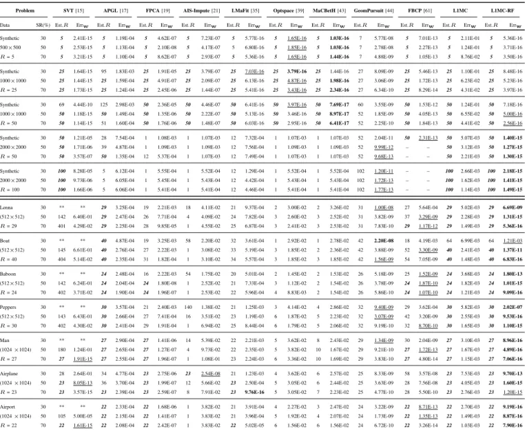
Table I
RECOVERYACCURACY(RSE)ANDTIMECOST(SECONDS)OFDIFFERENTCOMPLETIONMETHODS ONSYNTHETIC ANDREALDATA(SR=SAMPLE RATIO= 30%, 50%, 70% ). WE HIGHLIGHT THEBESTRESULTS INBOLDFONTS AND SECOND BEST RESULTS IN UNDERLINE.
Problem SVT[15] APGL[17] FPCA[19] AIS-Impute[21] LMaFit[35] Optspace[39] MaCBetH[43] GeomPursuit[44] FBCP[61] L1MC L1MC-RF
Data SR (%) RSE Time RSE Time RSE Time RSE Time RSE Time RSE Time RSE Time RSE Time RSE Time RSE Time RSE Time Synthetic 30 1.59E-13 12.2 1.24E-04 3.0 8.00E-07 46.6 7.52E-07 0.77 1.06E-14 0.2 4.57E-15 6.0 4.31E-15 0.8 3.20E-06 20.9 7.21E-13 90.7 2.18E-01 1.5 1.84E-14 5.1 500×500 50 1.31E-13 13.8 1.15E-04 2.6 4.27E-08 49.9 4.24E-07 1.15 1.03E-14 0.4 3.35E-15 4.6 4.85E-15 1.1 1.67E-06 34.1 2.31E-13 100.1 1.26E-01 1.1 1.23E-14 3.0
R= 5 70 1.07E-13 15.8 1.11E-04 2.4 5.39E-06 1.0 2.95E-07 1.70 8.93E-15 0.3 2.89E-15 5.6 3.56E-15 1.6 2.88E-07 80.7 1.07E-13 83.5 8.83E-02 1.0 1.02E-14 1.8 Synthetic 30 3.55E-13 96.0 4.12E-02 27.2 4.73E-05 4.5 4.12E-07 12.79 1.39E-14 1.8 2.39E-15 802.1 4.41E-15 13.6 1.30E-06 1185.6 5.86E-13 1423.6 1.19E-01 31.8 2.21E-14 52.6 1000×1000 50 4.31E-13 93.5 1.45E-03 11.9 2.34E-06 4.6 2.17E-07 13.64 8.31E-15 1.4 1.90E-15 776.9 3.07E-15 16.9 3.20E-07 2278.6 1.79E-13 1408.3 6.45E-02 19.4 1.45E-14 29.3
R= 25 70 6.28E-13 124.0 1.26E-04 11.6 8.11E-06 5.4 1.47E-07 18.57 9.59E-15 1.9 1.85E-15 722.9 1.34E-15 19.4 9.93E-08 1755.5 8.56E-14 1356.7 4.40E-02 12.7 1.13E-14 17.3 Synthetic 30 3.91E-09 468.8 3.18E-02 149.1 1.00E-04 8.1 5.36E-07 74.75 2.00E-14 4.1 5.98E-15 32028.2 6.00E-15 102.0 9.11E-07 1796.4 1.80E-12 6851.8 1.45E-01 66.3 2.91E-14 119.9 1000×1000 50 5.14E-13 221.0 1.62E-04 49.0 9.57E-06 8.6 2.40E-07 53.94 1.37E-14 2.5 3.37E-15 46723.0 2.61E-15 112.7 3.68E-07 2250.5 4.43E-13 1539.7 7.06E-02 29.0 1.71E-14 46.3
R= 50 70 7.69E-13 175.2 3.76E-03 30.6 2.17E-05 8.7 1.54E-07 70.85 1.10E-14 2.9 2.63E-15 58715.9 2.13E-15 117.0 1.15E-07 3079.3 1.96E-13 1460.0 4.59E-02 19.3 1.30E-14 26.4 Synthetic 30 1.66E-04 482.9 2.91E-02 60.0 4.65E-02 225.3 4.64E-02 13.07 3.95E-02 50.3 4.64E-02 1046.6 4.64E-02 30.8 8.15E-09 17226.9 4.21E-10 67412.9 2.91E-02 380.5 2.09E-14 460.0 2000×2000 50 3.19E-05 671.0 1.52E-02 50.9 4.64E-02 222.1 4.64E-02 19.11 3.91E-02 61.1 4.64E-02 1218.6 4.64E-02 45.1 2.63E-09 26333.8 – – 1.75E-02 164.4 1.41E-14 207.4
R= 50 70 8.89E-06 852.2 7.31E-04 62.9 4.15E-02 229.3 4.64E-02 26.50 3.90E-02 71.7 4.64E-02 1470.8 4.64E-02 57.2 6.20E-10 35139.0 – – 1.23E-02 88.6 1.03E-14 106.6 Synthetic 30 7.15E-04 1800.7 3.21E-02 83.7 3.31E-02 200.5 3.30E-02 9.61 5.25E-02 42.3 3.30E-02 993.1 3.30E-02 33.0 7.07E-09 33362.0 – – 2.12E-02 750.3 2.93E-14 999.8 2000×2000 50 1.20E-04 1542.7 3.20E-02 109.7 3.31E-02 246.2 3.30E-02 24.17 3.02E-02 74.1 3.30E-02 1499.7 3.30E-02 43.7 1.58E-10 45820.5 – – 1.29E-02 267.0 1.69E-14 335.6
R= 100 70 2.80E-05 1367.1 3.19E-02 92.4 3.31E-02 218.0 3.30E-02 25.94 3.01E-02 64.6 3.30E-02 1452.6 3.30E-02 51.7 1.34E-10 58936.6 – – 8.90E-03 126.3 1.10E-14 155.5
Lenna 30 ** ** 1.11E-03 78.7 7.73E-02 240.1 2.70E-01 10.96 6.61E-02 3.7 2.46E-01 47.9 2.57E-01 1.5 1.74E-06 154.5 2.59E-02 918.9 1.68E-02 45.1 8.33E-07 62.9 (512×512) 50 6.63E-01 8102.3 6.74E-04 29.8 3.94E-02 249.2 2.69E-01 1.83 4.40E-02 4.8 2.28E-01 62.6 2.25E-01 2.4 5.92E-07 186.7 2.97E-06 1274.7 6.21E-03 11.2 2.83E-14 19.5
R= 40 70 9.27E-02 487.8 5.71E-04 9.0 2.77E-02 15.7 2.99E-01 1.27 3.91E-02 5.8 2.19E-01 80.1 2.25E-01 3.2 1.31E-07 237.0 8.67E-10 1709.0 3.78E-03 4.8 1.87E-14 7.9 Boat 30 ** ** 2.82E-03 143.2 9.74E-02 223.7 1.78E-01 35.32 6.31E-02 4.3 2.42E-01 59.4 2.36E-01 1.1 3.20E-06 294.2 9.43E-02 544.0 3.44E-02 103.2 1.47E-02 136.4 (512×512) 50 6.78E-01 8021.5 1.01E-03 47.9 6.71E-02 249.4 2.47E-01 1.12 4.39E-02 5.9 1.94E-01 64.9 2.17E-01 2.1 1.07E-06 211.6 5.47E-06 1881.7 8.82E-03 14.3 1.99E-09 36.1
R= 29 70 1.13E-01 491.3 7.36E-04 14.4 7.80E-02 15.0 2.47E-01 1.34 3.76E-02 7.1 1.93E-01 71.8 1.93E-01 3.1 4.03E-07 240.1 4.41E-06 2337.3 4.65E-03 5.3 3.05E-14 12.8 Baboon 30 ** ** 8.52E-04 40.2 7.63E-02 162.0 1.57E-01 14.17 5.30E-02 3.7 1.72E-01 41.5 1.77E-01 0.8 7.45E-07 131.6 7.53E-07 675.4 1.25E-02 28.2 3.92E-11 41.2 (512×512) 50 6.39E-01 6332.8 5.92E-04 13.7 2.27E-07 83.0 2.24E-01 1.46 4.41E-02 5.3 1.51E-01 62.3 1.76E-01 1.1 4.38E-07 166.1 2.94E-07 789.0 5.27E-03 7.8 2.23E-14 12.8
R= 24 70 7.86E-02 408.0 5.21E-04 6.0 4.52E-05 9.8 2.24E-01 1.73 3.59E-02 6.6 1.33E-01 93.0 1.76E-01 1.3 1.17E-07 209.3 1.34E-07 1412.6 3.33E-03 3.6 1.64E-14 5.5 Peppers 30 ** ** 1.14E-03 109.2 7.95E-02 310.8 7.47E-02 106.76 7.41E-02 3.6 2.89E-01 62.6 2.45E-01 2.2 1.31E-06 113.8 1.10E-02 1135.7 1.82E-02 61.6 4.82E-07 29.0 (512×512) 50 6.65E-01 9098.9 6.75E-04 37.0 3.73E-02 297.6 1.84E-01 5.99 5.48E-02 5.1 1.96E-01 134.0 2.13E-01 3.4 4.76E-07 125.0 5.05E-06 1938.7 6.45E-03 15.7 3.06E-14 28.2
R= 30 70 9.31E-02 657.9 5.67E-04 12.9 3.17E-02 20.7 3.67E-01 2.06 4.46E-02 6.6 1.90E-01 178.4 2.04E-01 5.1 2.53E-07 155.8 3.64E-07 2151.7 3.89E-03 6.6 1.96E-14 11.0 Man 30 ** ** 6.01E-04 26.7 1.84E-04 48.0 2.27E-01 12.71 7.77E-02 13.0 2.74E-01 327.5 2.29E-01 15.4 6.70E-07 981.8 2.59E-06 4458.9 6.45E-03 271.3 3.06E-14 304.5 (1024×1024 ) 50 1.36E-01 103689.7 5.14E-04 19.1 3.97E-05 56.0 4.08E-01 7.14 7.25E-02 19.0 2.76E-01 472.5 1.86E-01 34.1 2.51E-07 1563.1 1.20E-12 9937.5 3.25E-03 84.3 1.73E-14 96.9
R= 27 70 1.45E-12 456.4 4.84E-04 17.3 4.19E-05 56.7 4.53E-01 5.63 6.71E-02 23.3 2.55E-01 765.8 1.85E-01 42.0 8.23E-08 2128.4 1.96E-13 8360.5 2.17E-03 34.2 1.10E-14 39.3 Airplane 30 4.16E-01 13056.8 2.46E-03 53.6 3.17E-04 38.1 5.33E-08 18.96 6.10E-02 10.3 2.74E-01 233.5 2.34E-01 13.4 2.22E-06 1282.3 1.77E-05 10311.3 1.57E-02 238.3 1.06E-10 283.4 (1024×1024 ) 50 1.03E-11 270.7 2.83E-03 24.6 4.51E-05 37.1 2.31E-01 13.45 1.04E-02 11.7 2.48E-01 386.9 2.23E-01 21.2 5.69E-07 2425.0 6.03E-05 5855.4 7.83E-03 107.0 2.00E-14 122.4
R= 23 70 2.36E-12 112.9 4.47E-04 12.1 4.59E-05 44.8 3.24E-01 14.03 1.01E-14 9.7 2.47E-01 431.5 2.12E-01 33.2 1.42E-07 2904.4 3.56E-07 3957.7 5.17E-03 54.9 1.50E-14 62.1 Airport 30 ** ** 5.69E-04 24.2 1.86E-04 38.7 2.75E-01 2.37 2.82E-02 33.6 2.14E-01 243.4 2.24E-01 7.9 6.81E-07 745.9 4.16E-12 2996.8 6.61E-03 215.7 2.59E-14 245.5 (1024×1024 ) 50 5.65E-04 27994.4 4.95E-04 13.0 3.05E-05 38.9 2.74E-01 4.29 2.71E-02 42.0 1.96E-01 381.6 2.04E-01 14.3 3.49E-07 1152.2 6.46E-13 7525.8 3.44E-03 78.8 1.56E-14 90.5
R= 22 70 6.86E-13 148.6 4.69E-04 13.1 4.02E-05 47.3 2.74E-01 6.26 3.32E-03 38.8 1.77E-01 601.2 1.77E-01 25.0 1.64E-07 1571.7 1.53E-13 6303.0 2.32E-03 37.9 1.14E-14 42.9
results on three small synthetic matrices (500 ×500 with
R = 5, 1000×1000 with R = 25, and 1000×1000 with
R = 50), though L1MC-RF gives results of one order lower
only. LMaFit obtains similar results as L1MC-RF on these smaller matrices. However, LMaFit, OptSpace and MaCBetH do not keep their good performance on the larger matrices
(2000×2000, R = {50,100}), where L1MC-RF is still the
winner and outperforms the second best (GeomPursuit and FBCP) by several orders of magnitude. Moreover, on these large matrices, GeomPursuit costs more than 10 hours in a few cases and FBCP fails to recover them within 48 hours in most cases.
On thereal-world images(total 21 cases), only L1MC-RF
consistently achieves the top two results in all cases except one
(Boat image with SR = 30%) where GeomPursuit obtains the
best result. GeomPursuit and FBCP achieve the second best results following L1MC-RF in 16 out of 21 cases, while they are more time consuming (about 10 and 45 times slower than L1MC-RF on average respectively). Moreover, FBCP needs
more memory. OptSpace and MaCBetH fail to recover these real-world images and estimate wrong ranks (as shown in Table II). LMaFit also does not work well in the 21 cases
except one (Airplane image with 70% observations) where it
achieves the smallest reconstruction error. In addition, SVT, APGL and AIS-Impute take the second place in a few cases while SVT often fails to converge if the observed entries are
fewer (e.g., SR≤30%).
In a nutshell, L1MC-RF has shown good recoverability: it outperforms the three decomposition-based methods as well as GeomPursuit and FBCP on average, and also achieves smaller reconstruction errors than the four nuclear norm minimization-based methods in all cases. For illustration, we show two
examples of recovering the Boat and Lenna images with50%
observations in Fig. 9.
2) Time Cost: In terms ofcomputational cost, L1MC-RF
is not the fastest while our focus here is accuracy and our implementation is not optimized for efficiency. It is worth noting that AIS-Impute is the fastest algorithm due to its
Table II
ESTIMATEDRANK(EST.R)ANDRELATIVE ERROR OFSINGULAR VALUES OFDIFFERENTMETHODS ONSYNTHETIC ANDREALDATA. WE HIGHLIGHT THECorrect Estimated RankINBOLDANDitalicFONTS,SMALLESTERRwRESULTS INBOLDFONTS AND SECOND SMALLESTERRwIN UNDERLINE.
Problem SVT[15] APGL[17] FPCA[19] AIS-Impute[21] LMaFit[35] Optspace[39] MaCBetH[43] GeomPursuit[44] FBCP[61] L1MC L1MC-RF
Data SR(%) Est.R Errw Est.R Errw Est.R Errw Est.R Errw Est.R Errw Est.R Errw Est.R Errw Est.R Errw Est.R Errw Est.R Errw Est.R Errw Synthetic 30 5 2.41E-15 5 1.19E-04 5 4.62E-07 5 7.23E-07 5 5.77E-16 5 1.65E-16 5 1.03E-16 7 5.77E-08 5 7.01E-13 5 2.11E-01 5 5.36E-16 500×500 50 5 2.53E-15 5 1.13E-04 5 2.10E-08 5 4.17E-07 5 6.80E-16 5 1.85E-16 5 1.03E-16 7 2.78E-08 5 2.27E-13 5 1.24E-01 5 3.71E-16
R= 5 70 5 3.21E-15 5 1.10E-04 5 8.62E-07 5 2.93E-07 5 5.36E-16 5 1.65E-16 5 1.44E-16 7 4.88E-09 5 1.05E-13 5 8.76E-02 5 3.50E-16 Synthetic 30 25 1.64E-15 95 1.83E-03 25 1.91E-05 25 3.79E-07 25 7.03E-16 25 3.79E-16 25 1.44E-16 27 8.09E-09 25 5.46E-13 25 1.10E-01 25 8.48E-16 1000×1000 50 25 1.44E-15 25 1.59E-04 25 4.91E-07 25 2.09E-07 25 6.13E-16 25 4.87E-16 25 1.98E-16 27 3.06E-09 25 1.72E-13 25 6.23E-02 25 5.23E-16
R= 25 70 25 1.73E-15 25 1.24E-04 25 2.45E-06 25 1.44E-07 25 5.41E-16 25 3.43E-16 25 2.34E-16 27 6.34E-10 25 8.29E-14 25 4.31E-02 25 3.97E-16 Synthetic 30 69 4.44E-10 125 2.98E-03 50 2.36E-05 50 4.46E-07 50 6.41E-16 50 3.97E-16 50 7.69E-17 60 3.55E-09 50 1.53E-12 50 1.24E-01 50 7.18E-16 1000×1000 50 50 1.18E-15 50 1.49E-04 50 1.35E-06 50 2.22E-07 50 5.13E-16 50 3.46E-16 50 8.97E-17 52 1.85E-09 50 4.05E-13 50 6.55E-02 50 5.00E-16
R= 50 70 50 1.14E-15 51 1.60E-04 50 1.76E-06 50 1.48E-07 50 6.03E-16 50 2.95E-16 50 6.41E-17 52 2.25E-10 50 1.84E-13 50 4.41E-02 50 2.56E-16 Synthetic 30 50 1.21E-05 28 7.54E-04 1 1.08E-03 1 1.07E-03 12 7.32E-04 1 1.07E-03 1 1.07E-03 52 2.04E-11 50 2.31E-13 50 5.07E-03 50 1.40E-15 2000×2000 50 50 1.71E-06 39 4.87E-04 1 1.09E-03 1 1.09E-03 12 7.56E-04 1 1.09E-03 1 1.09E-03 52 9.99E-12 – – 50 3.12E-03 50 1.27E-15
R= 50 70 50 3.57E-07 50 1.35E-04 12 5.37E-04 1 1.07E-03 12 7.49E-04 1 1.07E-03 1 1.07E-03 52 9.68E-13 – – 50 2.21E-03 50 1.30E-15 Synthetic 30 100 8.28E-05 5 6.12E-04 1 5.55E-04 1 5.52E-04 12 1.29E-04 1 5.52E-04 1 5.52E-04 102 1.20E-11 – – 100 2.66E-03 100 2.18E-15 2000×2000 50 100 9.73E-06 5 6.05E-04 1 5.45E-04 1 5.43E-04 12 4.42E-04 1 5.43E-04 1 5.43E-04 102 1.72E-13 – – 100 1.62E-03 100 1.41E-15
R= 100 70 100 1.66E-06 5 6.06E-04 1 5.41E-04 1 5.41E-04 12 4.46E-04 1 5.41E-04 1 5.41E-04 102 1.77E-13 – – 100 1.14E-03 100 1.49E-15
Lenna 30 ** ** 29 3.25E-04 19 2.21E-03 18 4.11E-02 21 9.37E-04 2 3.00E-02 2 3.26E-02 31 1.00E-08 27 5.64E-04 29 5.02E-03 29 6.69E-09 (512×512) 50 142 6.40E-01 29 2.47E-04 26 7.71E-04 4 4.09E-02 24 7.82E-04 3 2.60E-02 3 2.52E-02 31 3.82E-09 37 3.29E-09 29 2.28E-03 29 1.31E-15
R= 29 70 401 4.29E-02 29 2.25E-04 28 9.85E-05 1 4.55E-02 25 6.87E-04 3 2.41E-02 3 2.53E-02 31 7.83E-10 29 1.17E-12 29 1.49E-03 29 5.36E-16 Boat 30 ** ** 40 4.87E-04 19 3.25E-03 58 2.20E-02 32 3.61E-04 1 2.92E-02 1 2.78E-02 42 2.20E-08 18 4.19E-03 64 6.99E-03 64 1.21E-03 (512×512) 50 145 6.61E-01 40 2.76E-04 27 2.22E-03 1 3.08E-02 33 5.19E-04 3 1.85E-02 2 2.36E-02 42 3.88E-09 52 3.30E-09 40 2.41E-03 40 1.37E-11
R= 40 70 404 5.14E-02 40 2.35E-04 31 1.82E-04 1 3.10E-02 34 5.57E-04 3 1.85E-02 3 1.85E-02 42 1.56E-09 54 7.05E-09 40 1.48E-03 40 6.83E-16 Baboon 30 ** ** 24 2.48E-04 16 2.22E-03 54 1.75E-02 20 5.01E-04 2 1.45E-02 2 1.53E-02 26 5.18E-09 25 1.52E-09 24 3.68E-03 24 1.80E-13 (512×512) 50 142 6.24E-01 24 2.04E-04 24 1.80E-08 1 2.52E-02 21 7.33E-04 3 1.12E-02 2 1.54E-02 26 3.78E-09 24 1.87E-10 24 1.82E-03 24 1.01E-15
R= 24 70 402 3.71E-02 24 1.90E-04 24 1.96E-07 1 2.53E-02 22 5.96E-04 4 8.83E-03 2 1.54E-02 26 5.86E-10 24 1.07E-10 24 1.21E-03 24 9.09E-16 Peppers 30 ** ** 30 3.57E-04 21 2.40E-03 140 1.38E-02 21 1.25E-03 3 4.14E-02 4 2.86E-02 32 9.40E-09 29 3.62E-04 30 5.82E-03 30 2.02E-07 (512×512) 50 143 6.43E-01 30 2.66E-04 27 7.41E-04 16 3.51E-02 23 1.19E-03 6 1.87E-02 5 2.23E-02 32 3.07E-09 42 3.20E-09 30 2.55E-03 30 9.53E-16
R= 30 70 402 4.30E-02 30 2.41E-04 29 1.91E-04 1 6.94E-02 25 8.44E-04 6 1.79E-02 5 2.06E-02 32 9.19E-10 32 8.70E-10 30 1.65E-03 30 1.10E-15 Man 30 ** ** 27 2.90E-04 27 1.41E-06 14 5.39E-02 22 2.21E-03 5 3.62E-02 8 2.43E-02 29 1.34E-09 30 2.04E-09 27 3.10E-03 27 8.96E-16 (1024×1024) 50 180 1.24E-01 27 2.65E-04 27 1.27E-07 4 9.73E-02 22 2.35E-03 5 3.82E-02 10 1.67E-02 29 9.21E-10 27 1.72E-13 27 1.67E-03 27 4.89E-16
R= 27 70 27 1.91E-15 27 2.55E-04 27 1.96E-07 1 1.08E-01 23 2.24E-03 6 3.36E-02 10 1.69E-02 29 3.83E-10 27 4.80E-14 27 1.15E-03 27 7.06E-16 Airplane 30 28 2.64E-01 34 4.77E-04 23 2.75E-06 23 2.54E-08 21 1.23E-03 4 3.62E-02 6 2.57E-02 25 8.33E-09 58 3.57E-08 23 7.53E-03 23 9.70E-13 (1024×1024) 50 23 8.05E-13 36 3.70E-04 23 1.99E-07 12 5.66E-02 23 2.50E-04 5 3.05E-02 6 2.44E-02 25 3.63E-09 28 7.56E-08 23 4.05E-03 23 1.60E-15
R= 23 70 23 3.57E-15 23 2.39E-04 23 2.59E-07 8 7.91E-02 23 9.76E-16 5 3.05E-02 7 2.23E-02 25 4.77E-10 28 5.50E-10 23 2.76E-03 23 1.20E-15 Airport 30 ** ** 22 2.33E-04 22 1.68E-06 1 3.82E-02 21 3.91E-04 4 2.27E-02 3 2.47E-02 24 3.22E-09 22 8.71E-13 22 2.70E-03 22 9.19E-16 (1024×1024) 50 105 5.00E-05 22 2.15E-04 22 1.41E-07 1 3.83E-02 21 3.96E-04 5 1.92E-02 4 2.07E-02 24 1.73E-09 22 1.35E-13 22 1.49E-03 22 8.87E-16
R= 22 70 22 1.61E-15 22 2.08E-04 22 2.42E-07 1 3.83E-02 22 5.02E-05 6 1.56E-02 6 1.56E-02 24 6.72E-10 22 3.26E-14 22 1.03E-03 22 7.90E-16
C-mex programming. LMaFit and MaCBetH are faster than L1MC-RF since they use an efficient nonlinear successive
over-relaxation scheme and employ theminFuncsoftware for
acceleration, respectively. On the other hand, FBCP is the slowest among these completion methods. GeomPursuit is much slower than L1MC-RF in each case although it takes the most second best results, i.e., L1MC-RF is more than 89 times and 10 times faster than GeomPursuit on average on the synthetic and real matrices, respectively. Moreover, SVT and OptSpace are also slower than L1MC-RF especially in some
cases (e.g., on 1000×1000withR= 50), which is probably
due to their heavy SVD computation.
3) Rank Estimation: We also report the corresponding
estimated rank (Est.R) and relative error of singular values
(Errw) in Table II, where we highlighted thecorrect estimated
rank in bold and italic fonts, smallest Errw in bold fonts
and second smallest Errw in underline in each row. For the
methods without the rank estimation step, we compute the estimated ranks by SVD of the recovered matrices.
From Table II, we observe that: L1MC-RF (L1MC) success-fully determines the true ranks of the given incomplete images
in all 36 cases excepting one (Boat image with SR = 30%),
where L1MC does not have enough observations. GeomPursuit
performs best with the smallest Errwin this case, which results
in the best recovery result. L1MC can determine the true rank, while its weight vector (singular values) is far from the ground
truth (Errw>10−3), resulting in poor recovery performance.
This demonstrates the significance of ourrefinement strategy
in L1MC-RF: with the refinement strategy, L1MC-RF further
refines the factors and weights via R1MC to pursue an optimal solution for matrix completion. In other words, L1MC-RF not only can automatically estimate the true rank exactly but also obtain the true singular values. On the other hand, though GeomPursuit cannot obtain exact true ranks, it consistently
learns the singular values with small errors (Errw of order
less than 10−7), which leads to good recovery performance.
Moreover, FBCP does not always successfully determine the true rank but it also obtains the singular values with very small