Optimization
Vol. 00, No. 00, January 2009, 1–17
RESEARCH ARTICLE
Numerical Study of Augmented Lagrangian Algorithms for Constrained Global Optimization
Ana Maria A. C. Rocha∗ and Edite M. G. P. Fernandes
Department of Production and Systems, University of Minho, 4710-057 Braga, Portugal
(v1.0 released February 2011)
This paper presents a numerical study of two augmented Lagrangian algorithms to solve continuous constrained global optimization problems. The algorithms approximately solve a sequence of bound constrained subproblems whose objective function penalizes equality and inequality constraints violation and depends on the Lagrange multiplier vectors and a penalty parameter. Each subproblem is solved by a population-based method that uses an electromagnetism-like mechanism to move points towards optimality. Three local search procedures are tested to enhance the EM algorithm. Benchmark problems are solved in a performance evaluation of the proposed augmented Lagrangian methodologies. A comparison with other techniques presented in the literature is also reported.
Keywords:global optimization; augmented Lagrangian; electromagnetism-like mechanism; heuristics;
AMS Subject Classification: 90C30; 90C26; 90C56; 90C59
1. Introduction
This paper aims at analyzing the practical behavior of two augmented Lagrangian methodologies for continuous constrained global optimization, where the subprob-lems have bound constraints only and are solved by the electromagnetism-like mechanism, a stochastic population-based algorithm. The problem to be addressed has the form:
minf(x) subject to g(x)≤0, h(x) = 0, x∈Ω, (1) where f : Rn → R, g : Rn → Rp and h : Rn → Rm are nonlinear continuous functions and Ω ={x∈ Rn :lb≤x ≤ub}. We do not assume that the objective functionf is convex. There may be many local minima in the feasible region. This class of global optimization problems arises frequently in engineering applications. Specially for large scale problems, derivative-free and stochastic methods are the most well-known and used methods. When equality and inequality constraints are present in the optimization problem, one of the following categories of methods can be used. In the methods based on penalty functions, the constraints violation is combined with the objective function to define a penalty function. This function aims at penalizing infeasible solutions by increasing their fitness values propor-tionally to their level of constraints violation. Penalty functions require the use
∗Corresponding author. Email: [email protected]
ISSN: 0233-1934 print/ISSN 1029-4945 online c
2009 Taylor & Francis
DOI: 10.1080/0233193YYxxxxxxxx http://www.informaworld.com
of a positive penalty parameter that aims to balance function and constraint vio-lation values. The most popular penalty functions use static, dynamic, annealing or adaptive penalty updating schemes [2, 4, 8, 17, 19, 22]. An augmented La-grangian function is a penalty function that depends on a penalty parameter, as well as on the Lagrange multiplier vectors associated with the constraints of the problem. Augmented Lagrangians are common in deterministic type methods for global optimization [6, 7, 18], but rare when combined with heuristics that rely on a population of points to converge to the solution [1, 25, 27, 28]. The other category defines methods based on biasing feasible over infeasible solutions. They seem to be nowadays an interesting alternative to penalty methods for handling constraints. In this type of methods, constraints violation and the objective function are used separately and optimized by some sort of order, being the constraints violation the most important. See, for example, [9, 13, 20, 21, 23, 24, 29].
In this paper, we are interested in a penalty-type method that uses augmented Lagrangian methodologies to handle the equality and inequality constraints of the problem (1), where the subproblems are approximately solved by a stochastic global population-based algorithm. Due to its simplicity, the electromagnetism-like (EM) algorithm proposed in [4, 5] is used to obtain the solution of each subproblem. The EM algorithm simulates the electromagnetism theory of physics by considering each point in the population as an electrical charge. The method uses an attraction-repulsion mechanism to move a population of points towards optimality. Since the EM algorithm has been designed to find a minimizer which satisfies x ∈ Ω, our subproblem is defined as a bound constrained optimization problem.
The herein proposed implementation of an augmented Lagrangian methodology follows two paradigms. First, we apply the augmented Lagrangian function of Powell-Hestenes-Rockafellar (PHR) directly to the problem (1), and use the EM al-gorithm to solve the bound constrained subproblems. The EM alal-gorithm has been used within a classical penalty technique [4], but has not been used with an aug-mented Lagrangian function so far. Second, we reformulate problem (1) converting each equality constraint into an inequality as herein shown: |hj(x)| ≤ ε, where ε
is a positive relaxation parameter. This is an usual procedure in stochastic based methods [9, 14, 21, 22]. In general, the relaxation parameter is fixed over the entire iterative process. Typically, 10−3, 10−4 and 10−5 are common values in the litera-ture. Our proposal defines a sequence{εk}of decreasing nonnegative numbers such
that limk→∞εk=ε∗>0. The idea is to tighten the equality constraints relaxation
scheme as iterations proceed. Further, a different updating scheme for the penalty parameter is also proposed. When the level of constraints violation is under a specified tolerance, even if the infeasibility did not improve, the penalty is allowed to decrease instead of increasing (see Algorithm 2.2). In both cases, the bound constrained subproblems are approximately solved by the EM algorithm. This al-gorithm has been enhanced by a random local search procedure [5]. However, in practical terms, the therein proposed local search may require a large number of function evaluations since the local search is carried out along the coordinates. Attempting to reduce computational requirements while improving accuracy, two new local search procedures are herein proposed and tested to enhance the EM algorithm. One is based on the computation of a descent direction and the other relies on a unit-length randomly generated direction. We remark that there is no theoretical analysis yet for this algorithm.
The paper is organized as follows. Section 2 describes the two augmented La-grangian paradigms and Section 3 reviews the EM algorithm and presents the three local search procedures in comparison. Section 4 contains the results of all the nu-merical experiments, performance assessments based on Dolan and Mor´e’s profiles
[10], and a comparison with other methods in the literature. Finally, the remarks are included in Section 5.
2. Augmented Lagrangian methodologies
Most stochastic methods for global optimization are developed primarily for un-constrained or simple bound un-constrained problems. Then they are extended to constrained optimization problems using, for example, a penalty technique. This type of technique transforms the constrained problem into a sequence of uncon-strained subproblems by penalizing the objective function when constraints are vi-olated. The objective penalty function, in the unconstrained subproblem, consists of the objective functionf(x) plus a positive penalty parameter times a measure of the aggregate constraint violation. The choice of the penalty parameter may be problematic. In general, the penalty parameter is updated throughout the iterative process. With most penalty functions, the solution of the constrained problem is reached for an infinite value of the penalty parameter. An augmented Lagrangian is a more sophisticated penalty function for which a finite penalty parameter value is sufficient to yield convergence to the solution of the constrained problem [3].
Two augmented Lagrangian functions for solving constrained global optimization problems are now presented. Practical and theoretical issues from the augmented Lagrangian methodology are used with a stochastic population based algorithm, the EM algorithm [5], to compute approximate solutions of the sequence of bound constrained subproblems.
2.1. Handling equalities and inequalities separately
Our first proposal uses the original formulation (1) and makes use of the augmented Lagrangian function of Powell-Hestenes-Rockafellar (PHR):
LEIρ (x, λ, µ) =f(x) +ρ 2 m X i=1 hi(x) + λi ρ 2 + p X j=1 max 0, gj(x) + µj ρ 2 (2)
where λ ∈ Rm, µ ∈ Rp are the vectors of Lagrange multipliers associated with
h(x) = 0 andg(x)≤0 respectively, and ρ is a positive penalty parameter. For the sake of completeness we present in the Algorithm 2.1 the ideas presented in [7]. In this cited paper, the subproblems, at each iterationk,
min
x L
EI
ρk(x, λk, µk) subject to x∈Ω (3)
are approximately solved using a deterministic global optimization method known asαBB method.
According to recent works with the function (2) [6, 7], the penalty parameter is increased whenever the infeasibility is not reduced; otherwise it is not changed (see lines 7-11 in Algorithm 2.1). The initial value for the parameter is
ρ1 = max
10−6,min
10,2|f(x0)|/(kmax(0, g(x0))k2+kh(x0)k2)
for an arbitrary initial approximationx0. The algorithm also updates the Lagrange multipliers using first order estimates and safeguarded schemes (lines 12-13 in Al-gorithm 2.1). This is a crucial issue to maintain the sequences{λk},{µk}bounded.
Algorithm 2.1(Augmented Lagrangian algorithm)
1: Given:µ+>0,λ−< λ+,ǫ∗>0, 0< τ
c <1,γ >1,kmax,µ1∈[0, µ+],λ1∈[λ−, λ+]
2: choose arbitraryx0in Ω; computeρ1; setk= 1
3: whilemax{kvk−1k,kh(xk−1)k}> ǫ∗ andk≤k
max do
4: ǫk = max
ǫ∗,10−k ;
5: computexk, anǫk-global solution of min
xLEIρk(x, λk, µk) subject tox∈Ω 6: computevk j = max ( gj(xk),− µk j ρk ) , j= 1, . . . , p 7: if k= 1 or max{kvkk,kh(xk)k} ≤τ cmax{kvk−1k,kh(xk−1)k}then 8: ρk+1=ρk 9: else 10: ρk+1=γρk 11: end if 12: updateµk+1j = min max 0, µk j+ρkgj(xk), µ+ , j= 1, . . . , p 13: updateλk+1i = min max λ−, λk i +ρkhi(xk), λ+ , i= 1, . . . , m 14: k=k+ 1 15: end while
This paper aims at providing a different augmented Lagrangian algorithm that can be also implemented with the augmented Lagrangian functionLEI
ρ . The main
differences can be summarized as follows:
i) the initial approximation x0 is a randomly generated point;
ii) the subproblems (3) are solved by the EM algorithm, a stochastic algorithm based on a population of points, which uses the best solution found so far as the initial approximation to the subproblem of the next iteration;
iii) the penalty parameter ρ, besides being increased, is also reduced whenever the constraints violation is under a specified toleranceǫk, even if the level of
infea-sibility has increased.
Further, the penalty updating scheme herein used integrates a safeguarded scheme. This is motivated by the need to keep the penalty parameters bounded and the subproblems well conditioned. This procedure is reported in the lines 12–20 of the new Algorithm 2.2. With this algorithm, we aim to show the above mentioned differences, as well as the differences between using the formulation based on the Lagrangian (2) (translated in the Algorithm 2.1) and that based only on inequality constraints, as shown in (6). Issues related with the equality constraint relaxation parameter,εk, and details concerning the solving of subproblem (3) using the EM
algorithm are described in the next subsection.
2.2. Formulation based on inequality constraints
Since equality constraints are the most difficult to be satisfied, the other augmented Lagrangian methodology considers problems only with inequality constraints, using a common procedure in stochastic methods for global optimization to convert the equality constraints of the problem into inequality constraints, as follows:|hj| ≤ε,
j= 1, . . . , mfor a fixed ε >0. For simplicity, the problem (1) is rewritten as
minf(x) subject to G(x)≤0, x∈Ω, (4) where the vector of the inequality constraints is now defined by G(x) =
(g1(x), . . . , gp(x),|h1(x)| −ε, . . . ,|hm(x)| −ε). We now define t=p+m. Our
scheme as iterations proceed, using variable relaxation parameter values. Thus, a sequence of decreasing nonnegative values bounded byε∗ >0 is defined as:
εk+1 = max ε∗,1 γε k , γ >1. (5)
The PHR formula that corresponds to the inequality constraints in the converted problem (4) yields the augmented Lagrangian:
LIρ(x, µ) =f(x) +ρ 2 t X i=1 max 0, Gi(x) + µi ρ 2 (6)
where the Lagrange multiplier vector associated with the constraintsG(x)≤0,µ, has nowtelements.
Algorithm 2.2(Proposed augmented Lagrangian algorithm)
1: Given:µ+ >0,ǫ∗>0, 0< τ
c<1,γ >1,kmax,lmax,ε∗>0, 0< ρ−< ρ+,µ1∈[0, µ+]
2: randomly generate x0 in Ω; computeρ1; set k= 1
3: whilekvk−1k> ǫ∗ andk≤k
maxdo
4: ǫk= max
ǫ∗,10−k ; updateεk using (5); setl= 1
5: while LI
avg− LIρk(x(best), µk)
> ǫk andl≤l max do
6: usexk−1and randomly initialize a population ofp
size−1 points in Ω
7: run EM to compute a population of solutions to minxLIρk(x, µk) subject tox∈Ω
8: l=l+ 1 9: end while 10: xk=x(best) 11: computevk i = max Gi(xk),− µk i ρk , i= 1, . . . , t 12: if k= 1 orkvkk ≤τ ckvk−1kthen 13: ρk+1=ρk 14: else 15: if kvkk ≤ǫk then 16: ρk+1= max{ρ−,1 γρ k} 17: else 18: ρk+1= min{ρ+, γρk} 19: end if 20: end if 21: update µk+1i = min max 0, µk i +ρkGi(xk), µ+ , i= 1, . . . , t 22: k=k+ 1 23: end while
The herein proposed augmented Lagrangian algorithm adapted to the reformula-tion (4), of the original problem (1), and based on the Lagrangian (6) is presented in Algorithm 2.2. Lines 5-9 of the algorithm show details of the inner iterative pro-cess to compute an approximation to the solution of subproblem (3). Since the EM algorithm is based on a population of points, with sizepsize, the point which yields the least objective function value, denoted by the best point of the population,
x(best), after stopping, is taken as the next approximation to the problem (1). We also note that the stochastic EM algorithm uses the approximationxk−1 as one of the points of the population to initialize the EM algorithm. The remainingpsize−1 points are randomly generated.
The inner iteration counter is represented byl. This process terminates when the difference between the function value at the best point,LI
average of the function values of the population,LI
avg, is under a specified tolerance
ǫk. This tolerance decreases as outer iterations proceed. A limit of l
max iterations is also imposed.
3. The electromagnetism-like mechanism
This section reviews the electromagnetism-like mechanism, proposed in [5], for solving the subproblems in the Algorithm 2.2. In this algorithm context, an approximate minimizer of the augmented Lagrangian function, Lρk(x, µk), for
fixed values of the parameters ρk and µk is required. To simplify the notation,
Lk(x) = L
ρk(x, µk) will be used throughout the remainder of the paper. Because
EM is a population-based algorithm, the inner iterative process begins with a pop-ulation ofpsize solutions (line 6 in Algorithm 2.2). The best solution found so far, denoted by x(best), and the average of the objective function values, are defined by
x(best) = arg minnLk(x(s)) :s= 1, . . . , psize o and Lkavg= psize X s=1 Lk(x(s))/psize, (7) respectively, wherex(s), s= 1, . . . , psizerepresent the points of the population. The main steps of the EM mechanism are shown in Algorithm 3.1. Details of each step follow.
Algorithm 3.1(EM algorithm)
1: Given:x(s), s= 1, . . . , psize
2: evaluate the population and selectx(best) 3: compute the chargesc(s),s= 1, . . . , psize
4: compute the total forcesF(s),s= 1, . . . , psize
5: move the points exceptx(best)
6: evaluate the new population and selectx(best) 7: apply a local search tox(best)
8: compute Lk(x(best)) andLk avg.
The EM mechanism starts by identifying the best point, x(best), of the popula-tion using the augmented LagrangianLk for point assessment, see (7). According
to the electromagnetism theory, the total force exerted on each point x(s) by the otherpsize−1 points is inversely proportional to the square of the distance between the points and directly proportional to the product of their charges:
F(s) = psize X r6=s Fs r ≡ (x(r)−x(s)) c(s)c(r) kx(r)−x(s)k2,if L k(x(r))<Lk(x(s)) (x(s)−x(r)) c(s)c(r) kx(r)−x(s)k2,otherwise ,
fors= 1, . . . , psize, where the charge c(s) of point x(s) determines the magnitude
of attraction of that point over the others through
c(s) = exp −n L k(x(s))− Lk(x(best)) Ppsize r=1(Lk(x(r))− Lk(x(best))) ! .
Then, the normalized total force vector exerted on each point x(s) is used to move the point in the direction of the force by a random step size ι ∼ U[0,1], maintaining the point inside the set Ω. Thus fors= 1, . . . , psize (s6= best) and for each componenti= 1, . . . , n xi(s) = xi(s) +ι Fi(s) kF(s)k(ubi−xi(s)),if Fi(s)>0 xi(s) +ι Fi(s) kF(s)k(xi(s)−lbi), otherwise .
3.1. A random local search
Step 7 of Algorithm 3.1 aims at refining the search around the best point of the population only. A simple local search procedure proposed in [5], in the context of the EM algorithm, is described in Algorithm 3.2. This is a coordinatewise search applied tox(best). For each componenti,x(best) is assigned to a temporary point
y. Then a random movement of maximum length ∆ =δmaxj(ubj−lbj),δ >0, is
carried out and if a better position is obtained within maxlocal iterations,x(best)
is replaced byy, the search ends for that component and proceeds to another one. Wheny /∈Ω, the trial point is rejected and another random movement is tried for that component.
Although this local search is based on a simple random procedure, it has shown that improves accuracy of the EM algorithm although at a cost of function eval-uations. See the numerical study presented in Subsection 4.3 and the results in Table 1. To avoid the search along the coordinates, two other local search pro-cedures to enhance the EM algorithm in the augmented Lagrangian context are presented in the next subsections. One uses a descent direction for the augmented Lagrangian function and the other is based on a random direction.
Algorithm 3.2(Local search algorithm)
1: Given:x(best), maxlocal,δ
2: ∆ =δmaxj(ubj−lbj)
3: fori= 1 tondo
4: set it= 1
5: while it <maxlocal do
6: y←x(best)
7: yi=yi+ι∆, ι∼U[−1,1] (reject if not feasible)
8: if Lk(y)<Lk(x(best))then
9: x(best)←y,it= maxlocal−1
10: it=it+ 1 11: end while
12: end for
3.2. A descent local search
Here, a detailed description of a derivative-free heuristic method that produces an approximate descent direction and aims to generate a new trial point around the best point of the population is presented. In [12], a descent direction is proposed in a point-to-point search context, a simulated annealing method. It is shown that for a set of l exploring points close to x(best), an approximate descent direction may be produced if:
i) the points are randomly generated in a small neighborhood ofx(best) andl= 2, or
ii) the points are in equal distance tox(best), define withx(best) a set of orthogonal directions, andl=n.
For simplicity, case i) is implemented, and to produce a descent direction, two points in a neighborhood of ray δ > 0, of the best point, x(best), are randomly generated as follow:
xji(rand) =xi(best) +ι δ (i= 1, . . . , n), for j= 1,2 (8)
where ι ∼ U[−1,1] and δ is a sufficiently small positive value. The approximate descent directiond for the augmented Lagrangian functionLk, atx(best), is defined
by d=−P2 1 l=1|∆l| 2 X j=1 ∆j x(best)−xj(rand) kx(best)−xj(rand)k, (9)
where ∆j =Lk(x(best))−Lk(xj(rand)). A trial point is generated along the descent
direction with a prescribed step size,
y=x(best) +α d, (10)
where α ∈ (0,1] represents the step size. We remark that if y /∈ Ω, the point y
is projected onto the set Ω. When selecting a step size to detect a trial point y
that leads to an improvement inLk, when compared with the best point, the herein
proposed algorithm uses a classical backtracking strategy. Algorithm 3.3 presents a formal description of the descent local search. First, two random exploring points and a descent direction are generated. These two steps (lines 5-6) in the Algo-rithm 3.3 are executed wheneverflag is set to 1. Then, a trial pointyis calculated and, according to the augmented Lagrangian function values, either y or x(best) is selected. If x(best) still is the best point, then y is discarded, the step size is halved (i.e., α ← α/2) and a new point is evaluated along that descent direction (flag is set to 0 in the Algorithm 3.3). However, when y is the best, another ap-proximate descent direction is computed (flag is set to 1, and α is reset to 1) and the process is repeated. The search for a better point is implemented for at most maxlocal iterations. Practical performance of this descent search, when compared
with the other two local search procedures, is shown in Subsection 4.4.
3.3. A random walk
The random walk with direction exploitation method can be used as a local search procedure to refine the search around a particular point in the population. It has been applied as a local search operator to enhance a particle swarm optimization algorithm [19] and recently a differential evolution algorithm [16]. This random walk generates a random vector, as a search direction, and when applied to the best pointx(best) gives
y=x(best) +α z, (11)
where α ∈ (0,1] represents the step size and z is a unit-length random vector. The components ofzare randomly generated in the interval [−1,1]. The algorithm
Algorithm 3.3(Descent local search algorithm)
1: Given:x(best), maxlocal,δ
2: setflag = 1,α= 1,it= 0 3: whileit≤maxlocal do
4: if flag = 1then
5: generate two random points using (8) 6: compute descent directiondusing (9)
7: end if
8: compute trial pointy using (10) (project if not feasible) 9: if Lk(y)<Lk(x(best)) then 10: x(best)←y,α= 1, flag = 1 11: else 12: α=α/2,flag = 0 13: end if 14: it=it+ 1 15: end while
herein implemented projects the pointyonto the set Ω, when the point falls outside the bounds. Experiments have shown that this projection scheme is more efficient than the feasibility repair proposed in [16].
The random walk exploitation search can be summarized as the Algorithm 3.4 below. A backtracking strategy is also implemented. If y does not improve over
x(best), the step size is halved, and the random walk is tried again; otherwise, y
replacesx(best), α is reset to 1, and a new random walk is tried. Random walks can be tried for at most maxlocal iterations.
Algorithm 3.4(Random walk algorithm)
1: Given:x(best), maxlocal
2: setα= 1,it= 0 3: whileit≤maxlocal do
4: generate the random vector and compute pointy using (11) (project if not feasible) 5: if Lk(y)<Lk(x(best)) then 6: x(best)←y,α= 1 7: else 8: α=α/2 9: end if 10: it=it+ 1 11: end while 4. Numerical experiments
In this section, we report the results of our numerical study, after running a set of 24 benchmark constrained global problems, described in full detail in [15]. The problems are known as g01-g24 (the ‘g’ suit, where six problems only have equality constraints, thirteen have inequality constraints, five have both equalities and in-equalities and all have simple bounds). Not all problems have multi-modal objective functions, although some are difficult to solve. The best known solution for problem g20 is slightly infeasible. We remark that g02, g03, g08 and g12 are maximization problems that were transformed and solved as minimization ones. The C program-ming language is used in this real-coded algorithm that contains an interface to connect to AMPL and read the problems coded in AMPL [11]. The computational tests were performed on a PC with a 3GHz Pentium IV microprocessor and 1Gb of memory.
Since the algorithm relies on some random parameters and variables, we solve each problem 30 times and take average of the obtained solutions, herein denoted byfavg. The best of the solutions found after all runs is denoted byfbest. The size of the population depends on n, and since some problems have large dimension,
n > 20, we choose psize = min{200,10n}. The fixed parameters are set in this
study as follows:λ+ =µ+ =ρ+ = 1012,ǫ∗ = 10−6,τ
c = 0.5,γ = 2,λ− =−1012,
ε∗ = ρ− = 10−12, ε1 = 10−3. We define kmax = 50 and lmax = 30 so that a maximum of 1500 iterations are allowed. We remark that the other conditions in the stopping criteria of the Algorithm 2.2 (in the outer and inner iterative processes) may cause the termination of the algorithm before reaching the 1500 iterations. The initial multiplier vectors are set to the null vectors.
The values for the two parameters in the local search procedures are set as proposed in [5]: maxlocal = 10,δ = 0.001.
Overall, the algorithm with LI has nine parameters and with LEI has eleven
(including the two from the local search algorithm). The population size and the maximum number of allowed iterations are not counted as parameters since they are common to most population based techniques that we may use for comparison. Several tests were performed and some comparisons were carried out to choose appropriate values for some of the listed parameters.
4.1. Comparisons based on performance profiles
To compare the performance of the two augmented Lagrangian methodologies, and to analyze the effect of some parameters in the algorithm, we use performance profiles as described in Dolan and Mor´e’s paper [10]. Our profiles are based on the metrics: favg, the average of the solutions obtained at the end of each one of the 30 runs, and fbest, the best solution found in the 30 runs. Based on the chosen metric, these profiles compare the performance of a set of solvers, denoted byS, when solving a set of problems, here denoted by P. Let mp,s be the value of the
metric when solving problem p ∈ P by solver s∈ S. The comparison is based on the performance ratios defined by
rp,s = 1 +mp,s−min{mp,s:s∈ S},if min{mp,s:s∈ S}< β mp,s min{mp,s:s∈S},otherwise ,
where β is a positive small parameter [26]. We use β = 0.00001. The overall assessment of the performance of the solver s is given by ρs(τ) =
(no. of problems where rp,s ≤ τ)/(total no. of problems). Thus, ρs(τ) gives the
probability (for s ∈ S) that rp,s is within a factor τ ∈ R of the best possible
ratio. The value ofρs(1) gives the probability that a particular solver,s, will win
over the others in comparison. Thus, to just see which solver is the best, i.e., which solver has the least value of the metric mostly, thenρs(1) should be compared for
all the solvers. The higher theρs the better the solver is. On the other hand,ρs(τ)
for large values ofτ measures the solver robustness.
First, we carried out some tests to analyze the effect of the relaxation parameter choices in the context of the augmented Lagrangian LI
ρ(x, µ). Besides the usual
setting of a fixed value, for exampleε= 10−5, we implemented a variable update, as previously described in (5). The two penalty parameter updating schemes are also compared. The Figure 1 contains two plots. The plot (a) shows the performance profiles on the average performance, favg, of the four cases in comparison, herein denoted for convenience as:
1 1.1 1.2 1.3 1.4 1.5 1.6 1.7 1.8 0.3 0.4 0.5 0.6 0.7 0.8 0.9 1 τ ρ ( τ ) Performance profile on f avg 100 200 3000.8 0.82 0.84 0.86 0.88 0.9 0.92 0.94 0.96 0.98 1 τ ρ (orig) + ε fixed ρ (new) + ε fixed ρ (orig) + ε variable ρ (new) + ε variable (a) 1 1.02 1.04 1.06 1.08 1.1 1.12 1.14 1.16 1.18 0.4 0.5 0.6 0.7 0.8 0.9 1 τ ρ ( τ )
Performance profile on fbest
100 200 3000.8 0.82 0.84 0.86 0.88 0.9 0.92 0.94 0.96 0.98 1 τ ρ (orig) + ε fixed ρ (new) + ε fixed ρ (orig) + ε variable ρ (new) + ε variable (b)
Figure 1. Comparison of penalty and relaxation parameter updates based on: (a)favgand (b)fbest.
10 20 300.7 0.75 0.8 0.85 0.9 0.95 1 τ 1 1.002 1.004 1.006 1.008 1.01 0.5 0.55 0.6 0.65 0.7 0.75 0.8 0.85 0.9 0.95 1 τ ρ ( τ )
Performance profile on fbest
γ = 2 γ = 10 (a) 1 1.0001 1.0002 1.0003 1.0004 0.5 0.55 0.6 0.65 0.7 0.75 0.8 0.85 0.9 0.95 1 τ ρ ( τ )
Performance profile on fbest
5 10 150.8 0.82 0.84 0.86 0.88 0.9 0.92 0.94 0.96 0.98 1 τ k
max = 50 and lmax = 30
kmax = 30 and lmax = 50
(b)
Figure 2. Sensitivity analysis for: (a) the parameterγ; (b) different combinations ofkmaxandlmax.
• ρ (new) +ε fixed –ρ update according to Algorithm 2.2 andε= 10−5;
• ρ (orig) +εvariable –ρ update according to [7] andεupdate according to (5); • ρ (new) + ε variable – ρ update according to Algorithm 2.2 and ε update
ac-cording to (5).
Plot (b) shows the profiles on the best obtained solution over the 30 runs, fbest. We can conclude that the new proposed ρ updating scheme, combined with fixed
ε, outperforms the other combinations. Thus, this is the combination used in the remaining numerical tests.
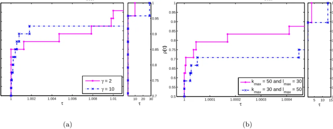
To analyze the effect of parameter γ, from the penalty parameter updating, as well as the effect of using less outer iterations and more inner iterations, while maintaining a maximum of 1500 iterations, on the performance of the algorithm, we use the augmented Lagrangian LI, and solve the ‘g’ suit. For the first set of
experiments, we testγ = 2 and γ = 10. From the plot on the left of Figure 2 we may conclude that the choice γ = 2 is slightly preferable. The profiles are based on the best performance of the algorithm, although a similar conclusion could be drawn from the average performance. The other plot, on the right, displays the profiles of the two cases in comparison:kmax= 50 and lmax= 30versus kmax= 30 and lmax = 50. Based on the best performance, the algorithm with the former choice is more effective in reaching the solution. (The same is true for the average performance.)
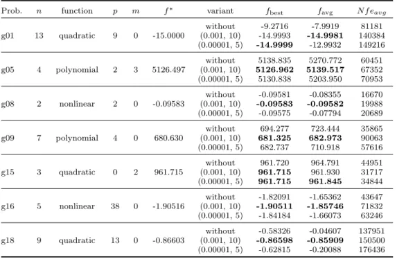
Table 1. EM without and with random local search defined by the pair (δ,maxlocal) .
Prob. n function p m f∗ variant fbest favg N f eavg
without -9.2716 -7.9919 81181 g01 13 quadratic 9 0 -15.0000 (0.001, 10) -14.9993 -14.9981 140384 (0.00001, 5) -14.9999 -12.9932 149216 without 5138.835 5270.772 60451 g05 4 polynomial 2 3 5126.497 (0.001, 10) 5126.962 5139.517 67352 (0.00001, 5) 5130.838 5203.950 70953 without -0.09581 -0.08355 16670 g08 2 nonlinear 2 0 -0.09583 (0.001, 10) -0.09583 -0.09582 19988 (0.00001, 5) -0.09575 -0.07794 20689 without 694.277 723.444 35865 g09 7 polynomial 4 0 680.630 (0.001, 10) 681.325 682.973 90063 (0.00001, 5) 682.737 710.918 57616 without 961.720 964.791 44951 g15 3 quadratic 0 2 961.715 (0.001, 10) 961.715 961.930 31717 (0.00001, 5) 961.715 961.845 34844 without -1.82091 -1.65362 43647 g16 5 nonlinear 38 0 -1.90516 (0.001, 10) -1.90511 -1.85746 71832 (0.00001, 5) -1.84184 -1.66073 63246 without -0.58326 -0.04607 137951 g18 9 quadratic 13 0 -0.86603 (0.001, 10) -0.86598 -0.85909 150500 (0.00001, 5) -0.62815 -0.20088 176436 4.2. Algorithm complexity
For completeness, the algorithm complexity, according to [15] is reported, using
T1= 1 N N X i=1 cpi, T2= 1 N N X i=1 ccpi, (12)
wherecpi andccpi represent the computing time (in seconds) of 10000 evaluations
of the basic functions (f,gandh) for problem i, and the complete computing time for the algorithm when 10000 evaluations of the functions are allowed, for problem
i, respectively, and N is the number of problems used in this computation. Using the ‘g’ suit (N = 24) and the augmented Lagrangian LI, we obtain:
T1= 0.0723, T2 = 0.8239 and (T2−T1)/T1 = 10.3956.
We remark that the displayed values are the average values over three runs and that the code was not yet optimized. We may conclude that the computational effort of the operations involved in the algorithm is about ten times the effort of evaluating the basic functions.
4.3. Random local search effect
Here, the effect of the random local search procedure (Algorithm 3.2) in the EM algorithm, is analyzed. Seven problems with different dimensions are selected: g01 with n = 13, g05 with n = 4, g08 with n = 2, g09 with n = 7, g15 with n= 3, g16 with n = 5 and g18 with n = 9. Each problem was solved 30 times. We run Algorithm 2.2 and selected the augmented LagrangianLI for this comparison.
Table 1 displays the problem (Prob.), the number of variables (n), the type of objective function (function), the number of inequality constraints (p), the number of equality constraints (m), the best known solution as reported in [15] (f∗), the
evaluations after the 30 runs). The three variants in comparison include one without local search and two with local search, each defined by the pair of parameters (δ,maxlocal). The accuracy of the obtained solutions is improved when the local
search is incorporated into the EM algorithm, although, as expected, at a cost of function evaluations. The choice (0.001, 10) for the pair of parameters is also better than the other in comparison. In all tables of the paper, the best results forfbest andfavg, in each table, are in boldface.
4.4. Comparing local search procedures
The random local search of Subsection 3.1 has an important limitation. Using it as described in Step 7 of Algorithm 3.1 can be time-consuming. It may require
nmaxlocal extra function evaluations, at each iteration. Its use seems impracticable
for moderate dimension problems. The proposals in Subsections 3.2 and 3.3 are more attractive since they look less expensive to implement and computational requirements do not depend on the problem dimension, as opposed to the case of random local search.
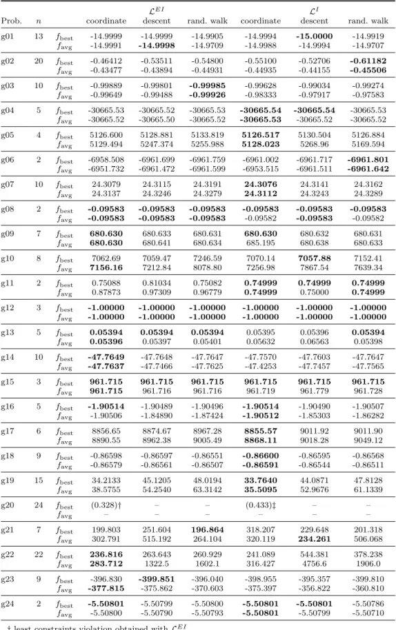
We run Algorithm 2.2 with both augmented Lagrangian functions, LEI and
LI, and tested the three local search procedures. In this study, the algorithm is
terminated when 100000 function evaluations are reached. Table 2 contains the results for the problems of the ‘g’ suit. The local search procedures are identified in the table by: ‘coordinate’ (Algorithm 3.2), ‘descent’ (Algorithm 3.3) and ‘rand. walk’ (Algorithm 3.4). The character ‘–’ means that the solution is infeasible. From the table we may conclude that Algorithm 3.2 slightly outperforms the other two in comparison, and the augmented Lagrangian LI attains, in general, the most
accurate results.
4.5. Comparison with other algorithms
To compare the performance of the herein proposed augmented Lagrangian al-gorithm with other penalty techniques in the literature [2, 17, 19], we report in Tables 3, 4 and 5 our results and those of the cited papers. In [2], a genetic algo-rithm (GA) combined with an adaptive penalty function (APF) is implemented. Five variants are tested. These are mainly concerned with the frequency of penalty parameters updating and constraints violation computation. The authors in [17] propose a momentum-type particle swarm optimization (PSO) algorithm combined with a dynamic penalty function (DPF) for solving constrained problems.
The method in [19] is a memetic particle swarm optimization (MPSO) algorithm, with a local search based on a random walk with direction exploitation (RW), and a dynamic penalty function. Both local and global variants are therein tested. To compare our results with the three chosen techniques, the problems were solved using the conditions described in the paper in comparison. These conditions are displayed in each table. They differ from one case to another and are concerned with psize, number of runs, and maximum number of iterations/generations or
function evaluations allowed. To identify the problem (‘Prob.’) we use the notation of the paper, except when the problem is of the ‘g’ suit or it has been used in a previous table. We report the results obtained with both augmented Lagrangians. The random local search procedure was chosen for these tests since it performed well in previous experiments.
Table 2. Comparison of local search procedures and augmented Lagrangians.
LEI LI
Prob. n coordinate descent rand. walk coordinate descent rand. walk g01 13 fbest -14.9999 -14.9999 -14.9905 -14.9994 -15.0000 -14.9919 favg -14.9991 -14.9998 -14.9709 -14.9988 -14.9994 -14.9707 g02 20 fbest -0.46412 -0.53511 -0.54800 -0.55100 -0.52706 -0.61182 favg -0.43477 -0.43894 -0.44931 -0.44935 -0.44155 -0.45506 g03 10 fbest -0.99889 -0.99801 -0.99985 -0.99628 -0.99034 -0.99274 favg -0.99649 -0.99488 -0.99926 -0.98333 -0.97917 -0.97583 g04 5 fbest -30665.53 -30665.52 -30665.53 -30665.54 -30665.54 -30665.53 favg -30665.52 -30665.50 -30665.52 -30665.53 -30665.52 -30665.52 g05 4 fbest 5126.600 5128.881 5133.819 5126.517 5130.504 5126.884 favg 5129.494 5247.374 5255.988 5128.023 5268.96 5169.594 g06 2 fbest -6958.508 -6961.699 -6961.759 -6961.002 -6961.717 -6961.801 favg -6951.732 -6961.472 -6961.599 -6953.515 -6961.511 -6961.642 g07 10 fbest 24.3079 24.3115 24.3191 24.3076 24.3141 24.3162 favg 24.3137 24.3246 24.3279 24.3112 24.3243 24.3289 g08 2 fbest -0.09583 -0.09583 -0.09583 -0.09583 -0.09583 -0.09583 favg -0.09583 -0.09583 -0.09583 -0.09582 -0.09583 -0.09582 g09 7 fbest 680.630 680.633 680.631 680.630 680.632 680.631 favg 680.630 680.641 680.634 685.195 680.638 680.633 g10 8 fbest 7062.69 7059.47 7246.59 7070.14 7057.88 7152.41 favg 7156.16 7212.84 8078.80 7256.98 7867.54 7639.34 g11 2 fbest 0.75088 0.81034 0.75082 0.74999 0.74999 0.74999 favg 0.87873 0.97309 0.96779 0.74999 0.75000 0.74999 g12 3 fbest -1.00000 -1.00000 -1.00000 -1.00000 -1.00000 -1.00000 favg -1.00000 -1.00000 -1.00000 -1.00000 -1.00000 -1.00000 g13 5 fbest 0.05394 0.05394 0.05394 0.05395 0.05396 0.05394 favg 0.05396 0.05397 0.05401 0.05632 0.06563 0.05398 g14 10 fbest -47.7649 -47.7648 -47.7647 -47.7570 -47.7603 -47.7647 favg -47.7637 -47.7466 -47.7625 -47.4253 -47.7457 -47.7565 g15 3 fbest 961.715 961.715 961.715 961.715 961.715 961.715 favg 961.715 961.716 961.716 961.719 961.779 961.728 g16 5 fbest -1.90514 -1.90489 -1.90496 -1.90514 -1.90490 -1.90507 favg -1.90506 -1.84890 -1.87424 -1.90512 -1.85303 -1.86282 g17 6 fbest 8856.65 8874.67 8967.28 8855.57 9011.92 9011.90 favg 8890.55 8962.38 9005.49 8868.11 9018.28 9049.12 g18 9 fbest -0.86598 -0.86597 -0.86551 -0.86600 -0.86595 -0.86568 favg -0.86579 -0.86561 -0.86507 -0.86591 -0.86544 -0.86511 g19 15 fbest 34.2133 45.1205 48.0194 33.7640 44.0871 47.8128 favg 38.5755 54.2540 63.3142 35.5095 52.9676 61.1339 g20 24 fbest (0.328)† – – (0.433)‡ – – favg – – – – – – g21 7 fbest 199.803 251.604 196.864 318.207 229.648 201.318 favg 302.791 515.192 264.104 320.119 234.261 506.068 g22 22 fbest 236.816 263.643 260.929 241.089 544.381 378.238 favg 283.712 1322.5 1602.1 316.427 4756.6 1906.0 g23 9 fbest -396.830 -399.851 -396.040 -398.955 -395.357 -399.810 favg -377.815 -375.862 -370.603 -375.397 -356.822 -360.810 g24 2 fbest -5.50801 -5.50799 -5.50800 -5.50801 -5.50801 -5.50786 favg -5.50800 -5.50790 -5.50793 -5.50801 -5.50799 -5.50710
†least constraints violation obtained withLEI. ‡least constraints violation obtained withLI.
Table 3 shows fbest and favg obtained by our study and those of [2] for the eleven problems therein reported (g01-g11). In [2] each variable was encoded with
Table 3. Comparison of our results with the best of 5 variants in [2].
Prob. f∗ our study [2]
Aug. Lagrangian fbest favg fbest favg
g01 -15.0000 LEI -14.9994 -14.9983 -14.9998 -14.9989 LI -14.9993 -14.9985 g02 -0.80362 LEI -0.57604 -0.43129 -0.79252 -0.72555 LI -0.49211 -0.33695 g03 -1.00050 LEI -0.99684 -0.99524 -0.99725 -0.77797 LI -0.99470 -0.97080 g04 -30665.54 LEI -30665.52 -30665.44 -30665.32 -30578.55 LI -30665.54 -30665.26 g05 5126.497 LEI 5128.380 5135.457 5126.779 5323.866 LI 5126.738 5130.937 g06 -6961.814 LEI -6950.783 -6896.591 -6961.448 -6805.229 LI -6954.896 -6910.745 g07 24.3062 LEI 24.3078 24.4817 24.5450 27.8486 LI 24.3070 24.3579 g08 -0.09583 LEI -0.09583 -0.09583 -0.09583 -0.08769 LI -0.09583 -0.09583 g09 680.630 LEI 680.630 680.645 680.681 681.470 LI 680.630 680.736 g10 7049.25 LEI 7098.94 8844.95 7070.56 8063.29 LI 7058.56 7147.76 g11 0.74990 LEI 0.74993 0.74998 0.75217 0.88793 LI 0.74999 0.75002
Conditions in [2]:psize= 100, runs = 25, maximum number of generations = 1000, leading to 100000 fitness function evaluations.
25 bits in a binary-coded GA. From the description of the algorithm in the paper, it is possible to identify three parameters in GA plus two in the procedure related with APF. We have better performance (both infbest andfavg) than the adaptive penalty algorithm of [2] in six problems.
Table 4 contains the results of our study to compare with the results reported in [17]. In the technique therein presented it is possible to identify four parameters in the PSO plus five in DPF. Since the algorithm was allowed to run for 5000 iterations, the solutions presented in this table may be better than those of the other tables. We have better performance (both infbest and favg) than [17] in two problems.
Finally, to compare with the dynamic penalty algorithm of [19], we register in Table 5 our results offavgand the corresponding standard deviation (Stand. Dev.), for the six problems listed in [19]. From the paper it is possible to identify three parameters in MPSO, plus two in RW and at least two in DPF. We obtain better
favg values in two problems and the other results are competitive.
A comparison based on the algorithms’ complexity cannot be carried out since the computing timesT1 andT2, see (12), are not provided in the papers [2, 17, 19].
5. Final remarks
From our preliminary numerical tests, we may conclude that the proposed aug-mented Lagrangian algorithm is able to effectively solve constrained problems till optimality. In particular, the augmented Lagrangian paradigm that uses relaxed equality constraints produces solutions with good accuracy. The augmented
La-Table 4. Comparison of our results with the results in [17].
Prob. f∗ our study [17]
Aug. Lagrangian fbest favg fbest favg
g02 -0.80362 LEI -0.46286 -0.42938 -0.80360 -0.746 LI -0.58645 -0.43610 g06 -6961.814 LEI -6959.716 -6948.447 -6961.814 -6961.781 LI -6957.870 -6933.025 g14 -47.7649 LEI -47.7616 -47.7600 -47.562 -46.604 LI -47.7544 -47.5938 P2 -31026.44 LEI -31026.42 -31026.40 -31025.56 -31025.56 LI -31026.42 -31026.38 P3 -11.0000 LEI -11.0000 -10.9535 -11.0000 -11.0000 LI -10.9999 -10.9998 P4 -213.000 LEI -213.000 -212.997 -213.000 -213.000 LI -213.000 -212.998
Conditions in [17]:psize= 50, runs = 20, maximum number of iterations = 5000.
Table 5. Comparison of our results with the best of the 2 variants in [19].
Prob. f∗ our study [19]
Aug. Lagrangian favg Stand. Dev. favg Stand. Dev. g04 -30665.54 LEI -30665.41 0.091 -30665.55 0.000 LI -30665.39 0.153 g06 -6961.814 LEI -6926.984 18.75 -6961.283 0.380 LI -6936.535 6.25 g09 680.630 LEI 680.631 0.0008 680.784 0.062 LI 680.631 0.0007 TP10 1.39347 LEI 1.40640 0.011 1.427 0.061 LI 1.39982 0.004 P2† -31026.44 LEI -31026.30 0.144 -31026.44 0.000 LI -31026.36 0.067 P4‡ -213.000 LEI -212.995 0.003 -213.047 0.002 LI -212.995 0.002
Conditions in [19]:psize= 100, runs = 30, maximum number of function evaluations = 100000.
†TP14 in [19];‡TP15 in [19].
grangian framework, coupled with the random local search procedure to enhance the EM algorithm, has shown to be competitive with other penalty based algo-rithms. The other two tested local search procedures did not improve significantly the final results. The convergence of the proposed algorithm will be carried out in the future. Other important issues, like the conditions for stopping the algorithm, will be analyzed.
Practical engineering problems, for example, those reported in [2], will be solved in the near future. We also aim to test our algorithms with a point-to-point search yet stochastic method, when solving the bound constrained subproblems.
Acknowledgments
The authors wish to thank two anonymous referees for their careful reading of the manuscript and their fruitful comments and suggestions.
References
[1] H.J.C. Barbosa,A coevolutionary genetic algorithm for constrained optimization, inProceedings of the 1999 Congress on Evolutionary Computation, DOI:10.1109/CEC.1999.785466, Vol. 3. (1999) pp. 1605–611.
[2] H.J.C. Barbosa and A.C.C. Lemonge, An adaptive penalty method for genetic algorithms in cons-trained optimization problems, inFrontiers in Evolutionary Robotics, H. Iba (ed.) 34 pages. 2008 (ISBN: 978-3-902613-19-6) I-Tech Education Publ., Austria.
[3] D.P. Bertsekas,Nonlinear Programming, 2nd edn. Athena Scientific, Belmont, 1999.
[4] S.I. Birbil,Stochastic Global Optimization Techniques, Ph.D. diss., North Carolina State University, 2002.
[5] S.I. Birbil and S.-C. Fang,An electromagnetism-like mechanism for global optimization, Journal of Global Optimization, 25 (2003), pp. 263–282.
[6] E.G. Birgin, R. Castillo, and J.M. Martinez,Numerical comparison of Augmented Lagrangian algo-rithms for nonconvex problems. Computational Optimization and Applications, 31 (2004), pp. 31-56. [7] E.G. Birgin, C.A. Floudas and J.M. Martinez, Global minimization using an Augmented La-grangian method with variable lower-level constraints, Mathematical Programming, Ser. A, DOI:10.1007/s10107-009-0264-y.
[8] C.A. Coello Coello,Use of a self-adaptive penalty approach for engineering optimization problems, Computers in Industry 41 (2000), pp. 113–127.
[9] K. Deb,An efficient constraint handling method for genetic algorithms, Computer Methods in Applied Mechanics and Engineering, 186 (1998), pp. 311–338.
[10] E.D. Dolan and J.J. Mor´e, Benchmarking optimization software with performance profiles, Mathe-matical Programming, 91 (2002), pp. 201–213.
[11] R. Fourer, D.M. Gay, and B.W. Kernighan,A modeling language for mathematical programming, Management Science, 36 (1990), pp. 519–554.
[12] A.R. Hedar and M. Fukushima,Heuristic pattern search and its hybridization with simulated anneal-ing for nonlinear global optimization, Optimization Methods and Software, 19 (2004) 291–308. [13] A.R. Hedar and M. Fukushima,Derivative-free filter simulated annealing method for constrained
continuous global optimization, Journal of Global Optimization, 35 (2006) 521–549.
[14] D. Karaboga and B. Basturk,Artificial Bee Colony (ABC) Optimization Algorithm for Solving Con-strained Optimization Problems,Lecture Notes In Artificial Intelligence, (P. Melin et al. (eds.)), Vol. 4529 (2007), pp. 789–798.
[15] J.J. Liang, T.P. Runarsson, E. Mezura-Montes, M. Clerc, P.N. Suganthan, C.A.C. Coello, and K. Deb, Problem definitions and evaluation criteria for the CEC2006 special session on constrained real-parameter optimization 2006. (http://www.ntu.edu.sg/home/EPNSugan/index files/CEC-06/CEC06.htm)
[16] T.W. Liao,Two hybrid differential evolution algorithms for engineering design optimization, Applied Soft Computing 10 (2010). pp. 1188–1199.
[17] J.-L. Liu and J.-H. Lin,Evolutionary computation of unconstrained and constrained problems using a novel momentum-type particle swarm optimization, Engineering Optimization 39 (2007), pp. 287–305. [18] H. Luo, X. Sun, and H. Wu,Convergence properties of augmented Lagrangian methods for constrained
global optimization, Optimization Methods and Software, 23 (2008), pp. 763–778.
[19] Y.G. Petalas, K.E. Parsopoulos, and M.N. Vrahatis,Memetic particle swarm optimization, Annals of Operations Research, 156 (2007), pp. 99–127.
[20] A.M.A.C. Rocha and E.M.G.P. Fernandes,Feasibility and dominance rules in the electromagnetism-like algorithm for constrained global optimization problems, Lecture Notes in Computer Science, Computational Science and Its Applications (O. Gervasi et al. (eds.)), Vol. 5073 (2008), pp. 768–783. [21] A.M.A.C. Rocha and E.M.G.P. Fernandes,Implementation of the electromagnetism-like algorithm with a constraint-handling technique for engineering optimization problems, in2008 Eighth Interna-tional Conference on Hybrid Intelligent Systems, ISBN: 978-0-7695-3326-1, IEEE Computer Society, (2008), pp. 690–695.
[22] A.M.A.C. Rocha and E.M.G.P. Fernandes,Self-adaptive penalties in the electromagnestism-like al-gorithm for constrained global optimization problems, inProceedings of the 8th World Congress on Structural and Multidisciplinary Optimization, CD 10 pages, Lisbon 2009.
[23] A.M.A.C. Rocha and E.M.G.P. Fernandes,Hybridizing the electromagnetism-like algorithm with de-scent search for solving engineering design problems, International Journal of Computer Mathematics, 86 (2009), pp. 1932–1946.
[24] T.P. Runarsson and X. Yao, Stochastic ranking for constrained evolutionary optimization, IEEE Transactions on Evolutionary Computation, 4 (2000), pp. 284–294.
[25] K. Sedlaczek and P. Eberhard,Augmented Lagrangian particle swarm optimization in mechanism design, Journal of System Design and Dynamics, 1 (2007), pp. 410–421.
[26] A.I.F. Vaz and L.N. Vicente,A particle swarm pattern search method for bound constrained global optimization, Journal of Global Optimization, 39 (2007), pp. 197–219.
[27] B.W. Wah and T. Wang,Efficient and Adaptive Lagrange-Multipliers, Journal of Global Optimiza-tion, 14 (1999), pp. 1–25.
[28] T. Wang and B.W. Wah,Handling inequality constraints in continuous nonlinear global optimization, inIntegrated Design and Process Science(1996), pp. 267–274.
[29] A.E.M. Zavala, A.H. Aguirre, and E.R.V. Diharce,Constrained optimization via particle evolutionary swarm optimization algorithm (PESO), inGECCO’05, (2005), pp. 209–216.
![Table 3. Comparison of our results with the best of 5 variants in [2].](https://thumb-us.123doks.com/thumbv2/123dok_us/9340015.2812501/15.892.155.680.90.550/table-comparison-results-best-variants.webp)
![Table 5. Comparison of our results with the best of the 2 variants in [19].](https://thumb-us.123doks.com/thumbv2/123dok_us/9340015.2812501/16.892.144.692.440.707/table-comparison-results-best-variants.webp)
