Property market modelling and forecasting: simple vs complex models

Property market modelling

and forecasting: simple

vs complex models

Arvydas Jadevicius and Simon Huston

Department of Real Estate, School of Real Estate and Land Management,

The Royal Agricultural University, Cirencester, UK

Abstract

Purpose – The commercial property market is complex, but the literature suggests that simple models can forecast it. To confirm the claim, the purpose of this paper is to assess a set of models to forecast UK commercial property market.

Design/methodology/approach – The employs five modelling techniques, including Autoregressive Integrated Moving Average (ARIMA), ARIMA with a vector of an explanatory variable(s) (ARIMAX), Simple Regression (SR), Multiple Regression, and Vector Autoregression (VAR) to model IPD UK All Property Rents Index. The Bank Rate, Construction Orders, Employment, Expenditure, FTSE AS Index, Gross Domestic Product (GDP), and Inflation are all explanatory variables selected for the research.

Findings – The modelling results confirm that increased model complexity does not necessarily yield greater forecasting accuracy. The analysis shows that although the more complex VAR specification is amongst the best fitting models, its accuracy in producing out-of-sample forecasts is poorer than of some less complex specifications. The average Theil’s U-value for VAR model is around 0.65, which is higher than that of less complex SR with Expenditure (0.176) or ARIMAX (3,0,3) with GDP (0.31) as an explanatory variable models.

Practical implications – The paper calls analysts to make forecasts more user-friendly, which are easy to use or understand, and for researchers to pay greater attention to the development and improvement of simpler forecasting techniques or simplification of more complex structures. Originality/value – The paper addresses the issue of complexity in modelling commercial property market. It advocates for simplicity in modelling and forecasting.

Keywords United Kingdom, Market, Property, Modelling, Complex, Simple Paper type Research paper

Property market modelling and forecasting

Property market modelling and forecasting is an indispensable activity in property investment (Mitchell and McNamara, 1997). The issue has been the subject of a number of studies. As a result, numerous models have been developed to forecast property markets (Brooks and Tsolacos, 2010). According to Harris and Cundell (1995, p. 76),

“the market crash which traumatised the property industry between 1991 and 1994 has led the institutions in particular to seek greater predictive input to their portfolio management and investment decisions”. As McDonald (2002) points out, after the 1980s property boom property researchers responded to the crisis situation, and as a result substantial progress has been made in property market research and forecasting. Though Tonelli et al. (2004, p. 1) argues that “numerous econometric models have been proposed for forecasting property market performance, but limited success has been achieved in finding a reliable and consistent model to predict property market movements”, property researchers, including McGough and Tsolacos (1995), Wheaton

et al. (1997), Barras (2009) and Bork and Moller (2012) suggest that the property market

338

Simple and complex models

According to Caminiti (2004, p. 992), models are “invaluable tools”. Models help users to develop a better understanding of complex systems, allow testing for possible scenarios, predicting outcomes, as well as they can assist in the setting of priorities. Byrne et al. (2010) add that models have been produced for a range of different reasons (i.e. to improve one’s understanding on the subject and its processes, to predict, forecast or explore possible scenarios, or to provide a basis for decision making).

Despite the benefits of models, many concerns are expressed regarding their application. STOWA/RIZA (1999) observes that extensive use of models increases the risk of inexpert use which as a result can lead to unreliable modelling outcomes. Similarly, Middlemis et al. (2000) comments that if the model is poorly designed, or it does not represent the system being modelled properly, all efforts to create the model are virtually in vain, or are likely to generate inaccurate forecasts. Subsequently, Jakeman et al. (2006) notes difficulties associated with models. According to the researcher, the use of models can bring unwanted outcomes due to “limitations, uncertainties, omissions and subjective choices in models” ( Jakeman et al., 2006, p. 603). The issue of model use and application is also addressed by Box and Draper (1987), Sterman (2002), and Mellor et al. (2003), to name but a few. These commentators suggest a more rigorous critique of the subject. According to Box and Draper (1987, p. 424), “essentially all models are wrong, but some are useful”. Following Mellor et al. (2003, p. 16), “models offer more hindrance than help”. As Sterman (2002, p. 525) states,

“all decisions are based on models, and all models are wrong”. For Sterman, failure is built in models as they are only a simplification, an abstraction of the system at no solid foundation. Moreover, Sterman claims that models are based on unreliable human perception and knowledge. However, despite all of this criticism, researchers including Parker et al. (2002) and Caminiti (2004) consider models to be assets rather than liabilities and essential elements in understanding and forecasting complex systems.

What is the difference between simple and complex models?

Chorley (1967) was perhaps the first to generate a modelling typology, but within sequential forecasting arena few direct comparisons of simple and complex models are available. What is more, the distinction between a simple or complex remains obscure (Buede, 2009). Many researchers, including Armstrong et al. (1984), Armstrong (1986), Wilkinson (1999), and Sterman (2002) refer to simple and complex models without providing working structural definitions.

Batty and Torrens (2001), on the other hand, define a complex system as, “an entity which is coherent in some recognisable way but whose elements, interactions, and dynamics generate structures admitting surprise and novelty which cannot be defined a priori” (Batty and Torrens, 2001, p. 2). According to Holland (1995), a “complex” or

“adaptive” model is one that maintains its composition and coherence through time. In case of the socio-economic environment, Allen and Strathern (2005) suggest that a simple model is a structure of fixed, predictable behaviour, while a complex one is a system in which a range of possible structural changes can appear. According to Buede (2009), complex, or as the author indicate, science-based models, usually require greater amounts of data, as well as a greater set of relationships.

In property, as in other fields of research, only minor references as to what constitute simple and complex models are discussed. According to Chaplin (1999), econometric models, which are considered as complex structures, differ from simple competitors as they include more variables and contain a greater number of estimations. Brooks and

Tsolacos (2000) suggest that simple Autoregressive structures (Long-Term-Mean and Random-Walk) constitute only part of a more complex Vector Autoregressive (VAR) system. According to Stevenson and McGarth (2003), more complex forecasting techniques, such as Bayesian VAR models, are better at forecasting as they offer more flexible forecasting process. What is more, Brooks and Tsolacos (2010) comment that time-series extrapolative models such as Exponential Smoothing or Autoregressive Integrated Moving Average (ARIMA) are atheoretical, which means that they are not based on any underlying economic theory. These models produce forecasts capturing only empirically relevant properties of selected time series. In contrast, econometric models, which are considered as being more complex structures, are based on the economic theory relevant to the subject.

As the evidence from this discussion suggests, the more complex analytical and econometric modelling structures are newer, include more variables, contain a greater number of estimations, and accounts for attributes of the external environment. In contrast, simple models constitute an uncomplicated combination of rules, a limited number of variables, in most cases they are of a fixed structure and usually extrapolate into the future from the past values of the time series itself. Lizieri’s (2009) classification of the real estate forecasting methods, puts Exponential Smoothing, Simple Regression (SR), Multiple Regression (MR) and ARIMA models into the simple forecasting techniques category. The econometric and VAR specifications constitute the more complex modelling structures.

Which models are better?

The question that needs to be asked however is whether complex forecasting structures are any better at forecasting than simple ones. This issue is debated within various scientific areas including environment, economics, and physiology.

In area of population forecasting, estimates of Dorn (1950) and Hajnal (1955) suggest that complex population forecasting models, which typically incorporate large amounts of inputs, become overly complicated, and thus produce poorer accuracy. Eberhardt (1987) also finds that simple differenced equation models for populations are functional in extracting trend from data. The more up-to-date evidence on simple vs complex models is present in Ahlburg (1995) and Rogers (1995). According to both commentators, regardless of continuing advancements in the field of population modelling and forecasting, the paradox is that simple growth models continue to outperform the more complex structures.

Armstrong’s et al. (1984) assessment of the relative accuracy of both complex and simple extrapolative methods suggests that simple methods (e.g. Exponential Smoothing) generate a comparable degree of accuracy to more complex ones (e.g. Box-Jenkins approach). In the subsequent paper, Armstrong (1986) produces a qualitative review of the forecasting methods of the period from 1960 to 1984. The author arrives at the same conclusion that forecasters should be in favour of simple forecasting techniques over the more complex econometric structures.

Clements and Hendry’s (2003) investigation into economic forecasting is also not in a favour of complex forecasting models. As the authors indicate, “although which model does best in a forecasting competition depends on how the forecasts are evaluated and what horizons and samples are selected, ‘simple’ extrapolative methods tend to outperform econometric systems” (Clements and Hendry’s, 2003, p. 304). More recent evidence from Buede (2009) suggests that although simple models contain a large variance in their predictions, complex models still have a large probability of producing

Property

market

modelling and

forecasting

339

340

wrong results. Orrell and McSharry (2009) also observe that, as models become more complex and parameterised, the number of elements they contain increases significantly. As a result, even small changes in these parameters can have significant ramifications on modelling outcomes. Certainly, the commentators appreciate that more parameterised models may fit historic data better and that their structure can be more flexible. However, such models are less helpful at predicting the future. Accordingly, Orrell and McSharry (2009) refer to Occam’s razor principle (cited in Standish, 2004, p. 256), which states that “entities should not be multiplied unnecessarily”. In other words, models should be as simple as possible with the minimum number of parameters. Subsequently, the researchers suggest that instead of developing a “model of everything”, one should aim in developing a set of models which could be adapted to a particular situation (Standish, 2004, p. 741).

A more recent argument for simplicity is so called “frugal innovation” approach. Pioneered by Prahalad (2006) and now becoming popular within the business and management community, this approach suggests that one should keep things simple and look for what people actually need (Immelt et al., 2009; Sehgal et al., 2010; Radjou

et al., 2012). The main principle of this approach is to produce ideas that are affordable

and flexible. Radjou et al. (2012, p. 4) call it “Jugaad Innovation”. This Hindi term translates as “an innovative fix; an improvised solution born from ingenuity and cleverness”. Jugaad is about doing more with less.

Outside the business research literature, Dawes (1979) offers probably the best critique of complex systems. According to Dawes, in most ways simple mechanical combinations of a few variables outperforms more complex MR or complex human judgements. Consequently, Kennedy (2002, p. 575) heightens the need for and the adoption of “Keep It Sensibly Simple” modelling approach. Kennedy borrows this terminology from Zellner (1991, p. 6), who recommends using “KISS” or “Keep It Sophisticatedly Simple” modelling style. As both authors indicate, simple specifications are just as good as complex empirical techniques. In his study Kennedy additionally refers to Wilkinson (1999, p. 601) who recommends “Choosing a Minimally Sufficient Analysis” approach. According to Wilkinson, the researcher should not use complex modelling technique only to impress external parties or to deflect the criticism. The commentator suggests that if the assumption and reasoning behind the application of simpler model is reasonable, so then one should use it.

Speaking about advantages of the complex models, the opposite findings are presented by Armstrong (1975), Pandy (2003), and Li et al. (2005). In his research, Armstrong (1975) comments that naïve (simple) forecasting structures are less accurate than causal (more complex) methods. Pandy’s (2003) investigation into muscle function in walking and comparison of two different models reveals that although a simple model can help to explain basic characteristics of movements, it tends to generate misleading results. According to Li et al. (2005), the Basic Structural Model specification performs better than less complex forecasting technique in the context of the international tourism demand modelling.

In the property forecasting literature, the evidence suggests that often simple models such as Exponential Smoothing, SR, or ARIMA specifications outperform more complex forecasting techniques, including VAR and econometric models, or generate highly comparable outcomes (Chaplin, 1999; Newell et al., 2002; Stevenson and McGarth, 2003). Newell et al. (2002) conclude that despite the increased complexity in property market modelling methodologies, simple methods often performs as well as complex econometric structures. In short, whilst it may be true that complex property

market modelling structures contain more variables and equations, consider elements of the external environment, and seem to fit historic data with greater accuracy, simple forecasting methods are often more accurate, or at least as accurate as complex structures. The other advantage of simple models is that they avoid “noise” which, as Makridakis (1988, p. 475) notes can infect the multiple sources of more complex models. Pant and Starbuck (1990, p. 442) also suggest that “more complex, subtle, or elegant techniques give no greater accuracy than simple, crude or naïve ones. More complex methods might promise to extract more information from data, but such methods also tend to mistake noise for information. As a result, more complex methods make more serious errors, and they rarely yield the gains they promised”. All this reinforces what Meehl (1954, p. 4) found more than half a century ago, that simple model specifications performed best despite the prejudice of, so called, experts for complex statistical algorithms which they considered, “operational, communicable, verifiable, public, objective, reliable, behavioural, testable, rigorous, scientific, precise, careful, trustworthy, experimental, quantitative, down-to-earth, hard-headed, empirical, mathematical, and sound”. Notwithstanding their superior performance, the same experts, dismissed simple modelling approaches, as “mechanical, atomistic, additive, cut and dried, artificial, unreal, arbitrary, incomplete, dead, pedantic, fractionated, trivial, forced, static, superficial, rigid, sterile, academic, oversimplified, pseudoscientific, and blind”.

Given all this, Mahmoud (1984) calls analysts to make forecasts more user-friendly, and for researchers to pay greater attention to the development and improvement of simpler forecasting techniques or simplification of more complex structures. Armstrong et al. (2013) advocate for conservatisms when forecasting. These propositions can be well generalised by Thoreau (1897, p. 144) who more than 100 years ago wrote:

“simplicity, simplicity, simplicity! I say let your affairs be as two or three and not a hundred or thousand […] simplify, simplify”.

Data and its acquisition

The dependent variable

The current research employs rental value growth rather than returns or yields as the dependent variable. Unlike returns, rent, or the growth in the price of space, captures both space-user and investors perspectives. Barras (1984), Scott (1996), Ball et al. (1998), and Baum and Crosby (2008) all argue that rent is the critical variable considered by analysts and other stakeholders. According to Barras (1984), developer profitability and ultimately building supply is underpinned largely by rent levels. Capital market players also monitor rents which, ceteris paribus, determine building value. For surveyors, building value is often estimated by rent capitalisation. For space users, demand is a function of commercial property rents as well as firm operational fundamentals like firm output and worker space requirements (Ball et al., 1998). As Ball

et al. (1998) explains, when office-based business grows, it employs more people and,

eventually, creates demand for more space. With fixed supply, rent rises. The process is in reverse when demand for office-using firm’s output falls. To summarise, rent brings the four key property markets (developer, financier, land market, and end user) into simultaneous equilibrium. Rent (and its determination) is therefore is considered the most important variable in property economics (Hendershott et al., 2002a).

Despite its prominence, rent is not the only dependent variable used in the field of commercial property market modelling and forecasting. Tsolacos’ (1995) study assessed retail rents determination factors. D’Arcy et al. (1999) investigated dynamics

Property

market

modelling and

forecasting

341

342

of Dublin office rental market. Karakozova (2004) examined office returns in Helsinki. Brooks and Tsolacos (2010) developed and econometric model of office yields in the UK. However, despite a degree of latitude, there is a strong case for using rents as the dependent variable.

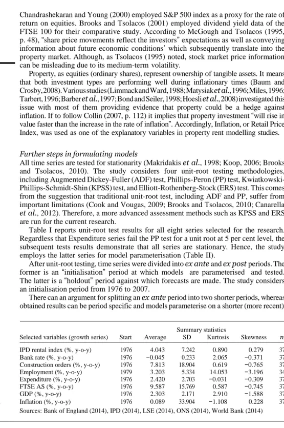
The research uses IPD All Property Rental Value Growth Index series for the UK. The index measures performance of directly held standing property investments from an open market valuations over the period from 1976 to 2012 (IPD, 2014). Certainly, IPD is not the only UK property market benchmark provider. Property consultancies including Jones Lang LaSalle (2014) and CBRE (2014) also produce UK commercial property indices. Nevertheless, IPD series is considered a reliable UK property market benchmarks by the investment and academic community (Baum, 2001; Ball, 2003; McAllister et al., 2005a, b; Piazolo, 2010; MacGregor et al., 2012; Drouhin and Simon, 2014). As of 2012, IPD data set contained 21,012 properties with a total capital value of £140.3 bn, including 559 purchases, 1,748 sales, and £18.6 bn in turnover (IPD, 2014) (Figure 1).

Explanatory variables

The subsequent analysis of research studies on commercial property market rent determination suggests that Bank Rate, Construction Orders, Employment, Expenditure, FTSE AS Index, Gross Domestic Product (GDP), and Inflation are all variables used to model UK commercial property rental dynamics. Certainly, series including Business Orders, Consumer Confidence, Floor-space, Index of Services, Retail Sales, Take-up, Business Turnover, Risk Premium, and Vacancy Rate were variables which property market researchers suggested as being relevant to model property rents. Unfortunately, data on these series was not available for such a long period of time or a special subscription was needed (Figures 2a and b).

The use of interest rates to model the commercial property market was argued by RICS (1994), Wheaton et al. (1997), Chaplin (1998), Orr and Jones (2003), Stevenson and McGarth (2003), and Qun and Hua (2009). According to researchers, interest rates do affect the commercial property, with higher interest rates depressing rental levels and vice versa.

Wheaton et al. (1997) and Matysiak and Tsolacos (2003) suggested using Construction Orders series as an explanatory variable. According to the commentators, this series can be employed as a potential leading indicator in forecasting rental series.

Figure 1. UK All Property Rental Index value growth (%, y-o-y) 25 20 15 10 5 0 –5 –10 –15 Source: IPD (2014)

IPD UK All Property Rental Value Growth (%)

1 9 7 6 1 9 7 8 1 9 8 0 1 9 8 2 1 9 8 4 1 9 8 6 1 9 8 8 1 9 9 0 1 9 9 2 1 9 9 4 1 9 9 6 1 9 9 8 2 0 0 0 2 0 0 2 2 0 0 4 2 0 0 6 2 0 0 8 2 0 1 0 2 0 1 2

(a) 50 40 30 20 10 0 –10 –20 –30 –40 (b) 50 40 30 20 10 0 –10 –20 –30 –40

Rent Expenditure Inflation Construction Orders

Rent Employment FTSE AS GDP Bank Rate

80 60 40 20 0 –20 –40 –60 –80 –100 0.80 0.60 0.40 0.20 0.00 –0.20 –0.40 –0.60 –0.80 –1.00

Property

market

modelling and

forecasting

343

Sources: (a) ONS (2014), LSE (2014); (b) Bank of England (2014), World Bank (2014)

Explanatory variables (%)

The Employment figures were used in various studies starting from an early publication of Hekman (1985) to those published more recently, e.g. Hendershott et al. (2008) and Qun and Hua (2009). In his research, Wheaton et al. (1997, p. 78) identified employment as “the primary instrument driving office space demand”.

The need to incorporate consumer expenditure into the property market modelling was argued by the RICS (1994), Tsolacos (1995), Hendershott (1996), Brooks and Tsolacos (2000), and Hendershott et al. (2002a, b). The significance of this variable was particularly emphasised within retail property studies suggesting a direct interrelationship between changes in levels of expenditure and commercial rents.

GDP was used in the number of studies, including Tsolacos (1995), Chaplin (1998), and Stevenson and McGarth (2003), as a measure of economic activity. As Stevenson and McGarth (2003) noted, GDP embodies economic growth in the whole economy which has a direct effect on the property market.

The empirical evidences suggest that stock market data can be successfully used for commercial property market modelling. McGough and Tsolacos (1995) included a share price index in their model to assess property cycles in the UK. Tsolacos (1995) used stock market data as an explanatory variable for industrial building investment.

1 9 7 6 1 9 7 8 1 9 8 0 1 9 8 2 1 9 8 4 1 9 8 6 1 9 8 8 1 9 9 0 1 9 9 2 1 9 9 4 1 9 9 6 1 9 9 8 2 0 0 0 2 0 0 2 2 0 0 4 2 0 0 6 2 0 0 8 2 0 1 0 2 0 1 2 1 9 7 6 1 9 7 8 1 9 8 0 1 9 8 2 1 9 8 4 1 9 8 6 1 9 8 8 19 90 1 9 9 2 1 9 9 4 1 9 9 6 1 9 9 8 2 0 0 0 2 0 0 2 2 0 0 4 2 0 0 6 2 0 0 8 2 0 1 0 2 0 1 2

344

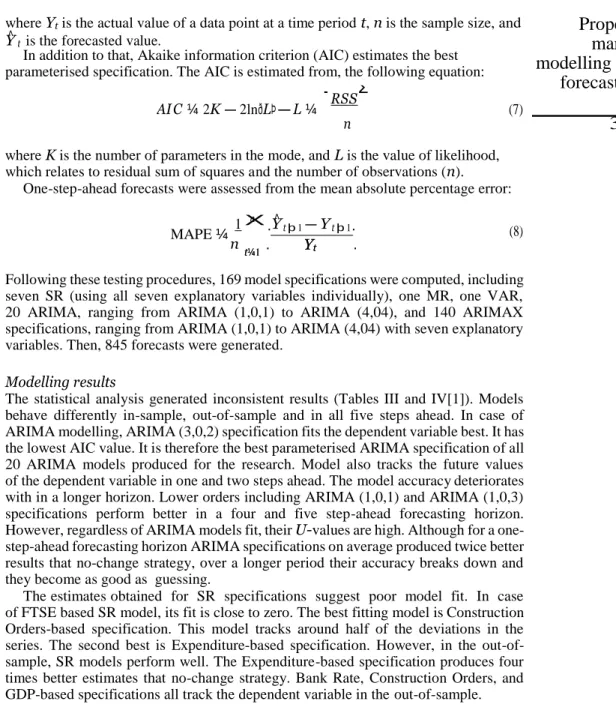
Chandrashekaran and Young (2000) employed S&P 500 index as a proxy for the rate of return on equities. Brooks and Tsolacos (2001) employed dividend yield data of the FTSE 100 for their comparative study. According to McGough and Tsolacos (1995, p. 48), “share price movements reflect the investors” expectations as well as conveying information about future economic conditions’ which subsequently translate into the property market. Although, as Tsolacos (1995) noted, stock market price information can be misleading due to its medium-term volatility.

Property, as equities (ordinary shares), represent ownership of tangible assets. It means that both investment types are performing well during inflationary times (Baum and Crosby, 2008). Various studies (Limmack and Ward, 1988; Matysiak et al., 1996; Miles, 1996; Tarbert, 1996; Barber et al., 1997; Bond and Seiler, 1998; Hoesli et al., 2008) investigated this issue with most of them providing evidence that property could be a hedge against inflation. If to follow Collin (2007, p. 112) it implies that property investment “will rise in value faster than the increase in the rate of inflation”. Accordingly, Inflation, or Retail Price Index, was used as one of the explanatory variables in property rent modelling studies.

Further steps in formulating models

All time series are tested for stationarity (Makridakis et al., 1998; Koop, 2006; Brooks and Tsolacos, 2010). The study considers four unit-root testing methodologies, including Augmented Dickey-Fuller (ADF) test, Phillips-Peron (PP) test, Kwiatkowski- Phillips-Schmidt-Shin (KPSS) test, and Elliott-Rothenberg-Stock (ERS) test. This comes from the suggestion that traditional unit-root test, including ADF and PP, suffer from important limitations (Cook and Vougas, 2009; Brooks and Tsolacos, 2010; Canarella

et al., 2012). Therefore, a more advanced assessment methods such as KPSS and ERS

are run for the current research.

Table I reports unit-root test results for all eight series selected for the research. Regardless that Expenditure series fail the PP test for a unit root at 5 per cent level, the subsequent tests results demonstrate that all series are stationary. Hence, the study employs the latter series for model parameterisation (Table II).

After unit-root testing, time series were divided into ex ante and ex post periods. The former is an “initialisation” period at which models are parameterised and tested. The latter is a “holdout” period against which forecasts are made. The study considers an initialisation period from 1976 to 2007.

There can an argument for splitting an ex ante period into two shorter periods, whereas obtained results can be period specific and models parameterise on a shorter (more recent)

Summary statistics

Selected variables (growth series) Start Average SD Kurtosis Skewness n

Table I. Series summary

statistics Sources: Bank of England (2014), IPD (2014), LSE (2014), ONS (2014), World Bank (2014) IPD rental index (%, y-o-y) 1976 4.043 7.242 0.890 0.279 37 Bank rate (%, y-o-y) 1976 −0.045 0.233 2.065 −0.371 37 Construction orders (%, y-o-y) 1976 7.813 18.904 0.619 −0.765 37 Employment (%, y-o-y) 1979 3.203 5.334 14.053 −3.196 34 Expenditure (%, y-o-y) 1976 2.420 2.703 −0.031 −0.309 37 FTSE AS (%, y-o-y) 1976 9.587 15.769 0.587 −0.745 37 GDP (%, y-o-y) 1976 2.303 2.171 2.910 −1.588 37 Inflation (%, y-o-y) 1976 0.089 33.904 −1.108 0.228 37

Property

market

modelling and

forecasting

345

Notes: The test critical values (significance is at 5 per cent level) are as follows: Augmented Dickey-Fuller (ADF) test: −2.874; Phillips-Peron (PP) test: −2.874; Kwiatkowski-Phillips-Schmidt-Shin (KPSS) test: 0.463; Elliott-Rothenberg-Stock (ERS) test: 3.185

Sources: a_{Kwiatkowski et al. (1992, p. 166),} b_{Elliott et al. (1996, p. 825)}

Table II. Unit-root test results for selected series

period would allow examining model performance for the different states of the economy. A natural division would then be period from 1997 to 2007, for which Bill (2013, p. 60) coined “boom, boom, bang” period. Despite Tony Blair’s promise that he would end booms and busts in the economy (Lee, 2009; Jones and Norton, 2013), the commercial property prices in the UK almost doubled during his term as Prime Minister. This then followed Global Financial Crisis (Shiller, 2008; Akerlof and Shiller, 2010), which subsequently pushed Britain into a recession which halved some property values (Bill, 2013).

At first compelling, this treatment creates more difficulties than it solves. First, the standard time-series modelling theory suggests that well parameterised time-series models require more than 50 observations (inter alia, Holden et al., 1991; McGough and Tsolacos, 1995; Tse, 1997; Yaffee and McGee, 2000; Brooks and Tsolacos, 2010). For regression models, 20 observations are needed (inter alia, Mouzakis and Richards, 2004). In terms of cycle analysis, as Yaffee and McGee (2000, p. 3) suggest, for proper parameter estimation and model building, time series should contain “enough observations”. Although there is no general agreement as to what “enough observations” is, Yaffee and McGee recommend that if a series is cyclical or seasonal, then it should be long enough to cover several cycles or seasons to allow researchers to specify them. Colloquially, Winston Churchill is linked to the necessity of profound historical perspectives to inform futures thinking (Kass and Hirsch, 2012). Given models are parameterised on data starting from 1997, this would cover a different era of British property market, subsequently disregarding significant British real estate corrections in 1970s (Barras, 1994) and 1990s (Gentle et al., 1994; Muellbauer and Murphy, 1997).

At the ex post period, forecasts are run for one, two, three, four, and five steps ahead. The rationale behind this particular separation is that it allows assessing the forecasting accuracy of each of the models for short- and long-run horizons.

Modelling and empirical estimates

The property market modelling is performed using SR, MR, VAR, ARIMA, and Autoregressive Integrated Moving Average with a vector of an explanatory variable(s) (ARIMAX) techniques. The use of these methods comes from classification of real estate forecasting methods presented in Lizieri (2009). Equations for each of these specifications are as follows.

Model test results

Series ADF PP KPSSa _ERSb

IPD rental series (%, y-o-y) −4.520 −2.600 0.280 0.580 Bank rate (%, y-o-y) −4.900 −4.140 0.350 0.750 Construction orders (%, y-o-y) −3.240 −2.990 0.400 2.630 Employment (%, y-o-y) −3.960 _−3.960 a 0.240 0.980 Expenditure (%, y-o-y) −3.090 −3.126 0.230 2.430 FTSE AS (%, y-o-y) −6.350 −6.340 0.430 1.710 GDP (%, y-o-y) −3.310 −3.270 0.150 1.960 Inflation (%, y-o-y) −6.320 −6.330 0.250 1.870

X v uP ffiffiffiffiffiffi n ffi — ffiffiffi 1 ffiffiffi_.ffiffi Y ffiffi ^ ffiffiffiffiffiffiffiffiffiffiffiffi Y ffiffiffiffiffiffiffiffiffiffiffi = ffiffi YffiffiffiffiffiΣffiffiffi2 ffiffi ¼ _P n—1 ._Y t

346

where Yt is the current value of the dependent variable, yt−p is past values of the variable itself, μ is constant term, ϕj is jth order autoregressive parameter, bj is jth moving average parameter, and utis the error term at a time period t.

ARIMAX specification:

n

Yt ¼ m þ f1yt—1þ f2yt—2þ . . . þ fp yt—pþ giXt—iþb1ut—1

i¼0

þb2ut—2þ . . . þbqut—qþut (2)

where Xtis a vector of explanatory variable(s).

SR specification:

Yt ¼ aþbxtþet (3)

where Ytis a dependent variable at a period t, xtis an explanatory variable at a period t, and etis an error term at the same period t.

MR specification:

Yt ¼ aþb1x1t þb2x3t þ . . . þbnxktþet (4)

where set of x1t, x2t, …, xktrepresents a group of explanatory variables, and set of β1, β2, …, βnis a group of regression coefficients at the time period t.

VAR specification:

Yt ¼ a1þ f11yt—1þ . . . þ f1pyt—pþ b11xt—1þ . . . þ b1pxt—pþe1t (5a)

Xt ¼ a1þ f11yt—1þ . . . þ f1pyt—pþ b11xt—1þ . . . þ b1pxt—pþ e1t (5b) This set of equations results is known as VAR (p) model. This specification has two variables, intercept, deterministic trend, and p lags of each of the variables (Koop, 2006). The research uses traditional model accuracy measures. The R2 _{assesses the} goodness-of-fit of each model. Theil’s second inequality coefficient U examines the out- of-sample performance of each specification. Theil’s U allows for a comparison between forecasting method and naïve modelling approach. According to Chaplin (1998, 1999) and Makridakis et al. (1998), if U is equal to zero, then predictions are perfect; if it is equal to one, then the forecasts are the same as those that would be obtained using naïve (no-change) forecasting approach; if, however, U is greater than one, then naïve (no-change) approach would produce better results and therefore there is no need for formal forecasting. The formula for U is as follows:

U ut t¼1 t þ 1— t þ 1 t (6) þ þ t¼1 þ þ 1—Yt ₁=Y_tΣ2

n AIC ¼ 2K — 2lnðLÞ-L ¼ . RSSΣ (7) MAPE ¼ n . . (8)

where Ytis the actual value of a data point at a time period t, n is the sample size, and

Y^ _{t is the forecasted value.}

In addition to that, Akaike information criterion (AIC) estimates the best parameterised specification. The AIC is estimated from, the following equation:

Property

market

modelling and

forecasting

where K is the number of parameters in the mode, and L is the value of likelihood, which relates to residual sum of squares and the number of observations (n).

One-step-ahead forecasts were assessed from the mean absolute percentage error:

347

1 X .Y^ t þ 1 — Yt þ 1.

Following these testing procedures, 169 model specifications were computed, including seven SR (using all seven explanatory variables individually), one MR, one VAR, 20 ARIMA, ranging from ARIMA (1,0,1) to ARIMA (4,04), and 140 ARIMAX specifications, ranging from ARIMA (1,0,1) to ARIMA (4,04) with seven explanatory variables. Then, 845 forecasts were generated.

Modelling results

The statistical analysis generated inconsistent results (Tables III and IV[1]). Models behave differently in-sample, out-of-sample and in all five steps ahead. In case of ARIMA modelling, ARIMA (3,0,2) specification fits the dependent variable best. It has the lowest AIC value. It is therefore the best parameterised ARIMA specification of all 20 ARIMA models produced for the research. Model also tracks the future values of the dependent variable in one and two steps ahead. The model accuracy deteriorates with in a longer horizon. Lower orders including ARIMA (1,0,1) and ARIMA (1,0,3) specifications perform better in a four and five step-ahead forecasting horizon. However, regardless of ARIMA models fit, their U-values are high. Although for a one- step-ahead forecasting horizon ARIMA specifications on average produced twice better results that no-change strategy, over a longer period their accuracy breaks down and they become as good as guessing.

The estimates obtained for SR specifications suggest poor model fit. In case of FTSE based SR model, its fit is close to zero. The best fitting model is Construction Orders-based specification. This model tracks around half of the deviations in the series. The second best is Expenditure-based specification. However, in the out-of- sample, SR models perform well. The Expenditure-based specification produces four times better estimates that no-change strategy. Bank Rate, Construction Orders, and GDP-based specifications all track the dependent variable in the out-of-sample.

Summary model fit statistics

Model specification In-sample 1-step 2-steps 3-steps 4-steps 5-steps AIC

ARIMA (3,0,2) 0.939 4.483

SR (expenditure) 126.2 0.117 0.129 0.202 0.256

Table III. The best performing model specifications

t¼1 Yt

4,0,4 0.934 4.833 451.6 0.897 0.868 0.817 0.728 0.952 4.521 493.4 0.930 0.881 0.858 0.809

(continued ) ARIMAX

Order

Bank rate Construction orders

In-sample Out-of-sample In-sample Out-of-sample

R2 _{AIC 1-step 2-steps 3-steps 4-steps 5-steps R}2 _{AIC 1-step 2-steps 3-steps 4-steps 5-steps}

1,0,0 0.647 5.968 316.5 0.816 0.801 0.713 0.608 0.727 5.711 6.325 0.289 0.428 0.439 0.417 1,0,1 0.862 5.094 315.0 0.827 0.818 0.737 0.636 0.851 5.171 404.7 0.937 0.872 0.832 0.747 1,0,2 0.872 5.082 273.1 0.846 0.826 0.731 0.622 0.847 5.118 554.4 0.940 0.902 0.871 0.796 1,0,3 0.884 4.864 279.6 0.787 0.787 0.712 0.616 0.821 5.486 108.2 0.688 0.639 0.623 0.576 1,0,4 0.919 4.754 292.6 0.807 0.798 0.715 0.617 0.882 5.133 503.9 0.904 0.871 0.860 0.815 2,0,0 0.887 4.932 414.7 0.911 0.877 0.812 0.717 0.877 5.023 490.6 0.942 0.884 0.856 0.799 2,0,1 0.910 4.774 378.8 0.903 0.870 0.799 0.695 0.882 5.043 531.7 0.945 0.901 0.873 0.810 2,0,2 0.910 4.839 383.3 0.902 0.871 0.871 0.697 0.886 5.076 530.0 0.945 0.898 0.870 0.809 2,0,3 0.929 4.676 414.1 0.890 0.866 0.809 0.713 0.904 4.969 510.4 0.926 0.874 0.848 0.794 2,0,4 0.924 4.801 386.7 0.890 0.867 0.803 0.706 0.902 5.059 222.2 0.529 0.600 0.609 0.558 3,0,0 0.900 4.911 393.1 0.899 0.873 0.807 0.707 0.879 5.104 511.5 0.943 0.895 0.868 0.809 3,0,1 0.909 4.880 376.8 0.901 0.870 0.799 0.696 0.912 4.846 513.5 0.932 0.880 0.856 0.805 3,0,2 0.914 4.894 319.2 0.876 0.854 0.766 0.656 0.913 4.911 515.1 0.931 0.878 0.854 0.804 3,0,3 0.923 4.856 586.6 0.929 0.902 0.866 0.793 0.913 4.979 510.9 0.930 0.877 0.853 0.802 3,0,4 0.930 4.824 439.3 0.900 0.883 0.832 0.747 0.913 5.045 518.3 0.934 0.880 0.856 0.805 4,0,0 0.905 4.910 429.2 0.922 0.885 0.827 0.738 0.886 5.100 525.0 0.939 0.896 0.871 0.817 4,0,1 0.908 4.959 402.0 0.913 0.879 0.816 0.719 0.906 4.979 512.7 0.932 0.880 0.855 0.804 4,0,2 0.953 4.348 304.5 0.828 0.828 0.774 0.684 0.953 4.355 449.9 0.929 0.868 0.841 0.786 4,0,3 0.949 4.515 436.0 0.918 0.888 0.834 0.744 0.870 5.443 274.8 0.668 0.656 0.647 0.621

JP

IF

3

3

,4

34

8

ARIMAX Order

Employment Expenditure

In-sample Out-of-sample In-sample Out-of-sample

R2 _{AIC 1-step 2-steps 3-steps 4-steps 5-steps R}2 _{AIC 1-step 2-steps 3-steps 4-step 5-steps}

1,0,0 0.648 6.011 500.4 0.927 0.911 0.875 0.797 0.672 5.896 231.9 0.785 0.727 0.708 0.618 1,0,1 0.820 5.411 397.9 0.948 0.918 0.878 0.794 0.832 5.289 177.6 0.967 0.850 0.800 0.690 1,0,2 0.885 5.034 524.5 0.942 0.915 0.879 0.797 0.878 5.035 603.2 0.957 0.927 0.894 0.819 1,0,3 0.874 5.201 396.1 0.930 0.883 0.839 0.754 0.884 5.051 479.1 0.951 0.917 0.880 0.797 1,0,4 0.941 4.507 474.5 0.922 0.912 0.896 0.845 0.871 5.221 305.2 0.948 0.900 0.859 0.767 2,0,0 0.854 5.203 557.4 0.948 0.919 0.888 0.816 0.860 5.149 492.5 0.944 0.907 0.875 0.798 2,0,1 0.870 5.163 493.3 0.944 0.915 0.880 0.799 0.873 5.118 447.9 0.942 0.904 0.867 0.778 2,0,2 0.871 5.227 491.2 0.947 0.916 0.880 0.799 0.877 5.156 409.3 0.946 0.899 0.860 0.771 2,0,3 0.894 5.108 515.1 0.936 0.909 0.876 0.801 0.892 5.086 421.6 0.916 0.881 0.849 0.770 2,0,4 0.883 5.276 286.6 0.973 0.936 0.863 0.758 0.935 4.643 600.5 0.964 0.911 0.873 0.795 3,0,0 0.860 5.276 534.7 0.945 0.918 0.888 0.814 0.867 5.195 509.5 0.945 0.914 0.883 0.807 3,0,1 0.870 5.284 489.9 0.945 0.916 0.880 0.798 0.899 4.992 500.7 0.936 0.866 0.836 0.754 3,0,2 0.893 5.159 474.1 0.942 0.916 0.884 0.809 0.901 5.035 610.7 0.945 0.910 0.882 0.806 3,0,3 0.901 5.161 460.8 0.933 0.920 0.906 0.868 0.905 5.066 626.9 0.951 0.914 0.886 0.815 3,0,4 0.951 4.540 464.2 0.909 0.887 0.852 0.792 0.941 4.660 623.9 0.960 0.912 0.877 0.803 4,0,0 0.869 5.347 542.6 0.949 0.919 0.887 0.814 0.874 5.197 469.3 0.941 0.905 0.875 0.800 4,0,1 0.873 5.392 489.4 0.945 0.914 0.877 0.795 0.881 5.216 399.8 0.937 0.895 0.859 0.772 4,0,2 0.915 5.080 539.7 0.918 0.901 0.867 0.792 0.911 4.997 422.1 0.934 0.910 0.891 0.834 4,0,3 0.939 4.818 510.4 0.903 0.890 0.858 0.786 0.911 5.060 409.9 0.933 0.908 0.889 0.829 4,0,4 0.891 5.486 283.8 0.964 0.937 0.855 0.743 0.914 5.100 398.3 0.934 0.906 0.884 0.821 (continued )

Pr

operty

market

modelling and

for

ec

as

ting

34

9

4,0,4 0.956 4.420 564.6 0.933 0.904 0.867 0.789 0.917 5.070 44.05 0.411 0.442 0.438 0.453

(continued ) ARIMAX

Order

FTSE GDP

In-sample Out-of-sample In-sample Out-of-sample

R2

AIC 1-step 2-steps 3-steps 4-steps 5-steps R2

AIC 1-step 2-steps 3-steps 4-steps 5-steps

1,0,0 0.614 6.059 613.0 0.925 0.899 0.864 0.787 0.649 5.962 176.4 0.448 0.499 0.502 0.469 1,0,1 0.856 5.138 560.0 0.912 0.893 0.862 0.794 0.844 5.215 8.300 0.407 0.442 0.443 0.420 1,0,2 0.910 4.736 441.8 0.853 0.832 0.788 0.703 0.915 4.676 307.0 0.923 0.820 0.774 0.689 1,0,3 0.910 4.800 439.5 0.851 0.831 0.785 0.700 0.963 3.918 346.0 0.809 0.767 0.734 0.672 1,0,4 0.879 5.156 595.1 0.911 0.892 0.858 0.784 0.901 4.953 189.9 0.580 0.584 0.575 0.512 2,0,0 0.870 5.075 635.0 0.925 0.900 0.868 0.797 0.876 5.028 318.2 0.838 0.765 0.730 0.662 2,0,1 0.903 4.847 524.3 0.912 0.886 0.843 0.755 0.892 4.955 237.8 0.754 0.702 0.666 0.588 2,0,2 0.905 4.899 521.3 0.923 0.892 0.850 0.764 0.894 5.008 36.93 0.539 0.552 0.541 0.487 2,0,3 0.931 4.643 477.7 0.874 0.848 0.803 0.717 0.927 4.692 350.6 0.685 0.677 0.660 0.634 2,0,4 0.937 4.616 627.9 0.919 0.896 0.861 0.787 0.944 4.500 324.5 0.925 0.821 0.775 0.690 3,0,0 0.881 5.086 602.0 0.920 0.897 0.864 0.790 0.886 5.046 296.3 0.805 0.749 0.713 0.645 3,0,1 0.913 4.838 486.6 0.915 0.890 0.847 0.759 0.893 5.046 224.2 0.750 0.699 0.662 0.585 3,0,2 0.919 4.835 469.2 0.913 0.886 0.842 0.756 0.897 5.080 48.38 0.278 0.322 0.339 0.324 3,0,3 0.921 4.888 473.5 0.904 0.885 0.847 0.765 0.919 4.905 10.46 0.285 0.304 0.303 0.331 3,0,4 0.934 4.766 513.6 0.889 0.870 0.835 0.760 0.925 4.897 93.64 0.321 0.371 0.378 0.368 4,0,0 0.896 5.007 616.0 0.921 0.897 0.864 0.796 0.893 5.038 280.2 0.798 0.736 0.702 0.639 4,0,1 0.912 4.906 508.6 0.906 0.880 0.837 0.752 0.895 5.090 255.8 0.781 0.724 0.687 0.617 4,0,2 0.920 4.891 571.4 0.910 0.885 0.849 0.773 0.894 5.167 155.1 0.558 0.563 0.547 0.502 4,0,3 0.932 4.794 452.2 0.867 0.846 0.793 0.793 0.894 5.235 154.6 0.566 0.570 0.553 0.506

JP

IF

3

3

,4

35

0

ARIMAX Order

Inflation

In-sample Out-of-sample ARIMA

R2 _{AIC 1-step 2-steps 3-steps 4-steps 5-steps Order}

In-sample Out-of-sample

R2 _{AIC 1-step 2-steps 3-steps 4-steps 5-Steps}

1,0,0 0.622 6.037 625.9 0.915 0.880 0.849 0.789 1,0,0 0.609 6.008 522.2 0.951 0.917 0.881 0.800 1,0,1 0.893 4.835 532.2 0.963 0.917 0.878 0.796 1,0,1 0.892 4.784 536.0 0.965 0.919 0.880 0.798 1,0,2 0.892 4.910 514.7 0.970 0.927 0.888 0.802 1,0,2 0.862 5.093 578.5 0.944 0.914 0.882 0.804 1,0,3 0.881 5.075 453.7 0.954 0.921 0.886 0.804 1,0,3 0.883 4.991 450.3 0.951 0.915 0.873 0.788 1,0,4 0.884 5.112 470.8 0.951 0.916 0.878 0.795 1,0,4 0.908 4.823 566.7 0.958 0.921 0.886 0.806 2,0,0 0.857 5.169 577.4 0.950 0.916 0.886 0.817 2,0,0 0.857 5.105 561.6 0.953 0.920 0.889 0.818 2,0,1 0.871 5.134 499.1 0.954 0.921 0.885 0.801 2,0,1 0.871 5.070 513.6 0.950 0.917 0.882 0.801 2,0,2 0.883 5.105 465.0 0.974 0.947 0.916 0.829 2,0,2 0.872 5.126 507.5 0.953 0.917 0.882 0.803 2,0,3 0.899 5.021 586.9 0.934 0.913 0.890 0.830 2,0,3 0.900 4.951 552.7 0.938 0.915 0.888 0.821 2,0,4 0.897 5.109 549.4 0.936 0.911 0.883 0.812 2,0,4 0.925 4.729 559.3 0.963 0.921 0.885 0.807 3,0,0 0.867 5.194 549.4 0.944 0.914 0.884 0.814 3,0,0 0.867 5.130 534.9 0.948 0.919 0.889 0.815 3,0,1 0.900 4.980 416.5 0.972 0.953 0.925 0.829 3,0,1 0.873 5.147 481.6 0.951 0.917 0.881 0.798 3,0,2 0.873 5.289 471.3 0.976 0.949 0.918 0.830 3,0,2 0.939 4.483 447.3 0.933 0.916 0.894 0.829 3,0,3 0.905 5.065 596.8 0.958 0.923 0.894 0.822 3,0,3 0.936 4.610 463.7 0.930 0.917 0.901 0.846 3,0,4 0.907 5.109 407.3 0.971 0.952 0.924 0.827 3,0,4 0.911 5.003 567.3 0.943 0.914 0.885 0.815 4,0,0 0.872 5.214 526.3 0.955 0.925 0.895 0.822 4,0,0 0.871 5.148 538.3 0.950 0.919 0.889 0.818 4,0,1 0.948 4.387 442.8 0.964 0.936 0.902 0.812 4,0,1 0.876 5.185 493.1 0.948 0.916 0.882 0.804 4,0,2 0.934 4.687 424.6 0.961 0.947 0.927 0.842 4,0,2 0.910 4.929 460.2 0.940 0.916 0.893 0.832 4,0,3 0.894 5.242 431.9 0.972 0.952 0.925 0.831 4,0,3 0.910 5.004 478.2 0.942 0.917 0.893 0.828 4,0,4 0.961 4.318 382.7 0.966 0.936 0.900 0.806 4,0,4 0.902 5.162 607.5 0.948 0.916 0.889 0.821 (continued )

Pr

operty

market

mode

lling and

for

ec

as

ting

35

1

Downloaded by Royal Agricultural University At 06:12 15 January 2019 (PT)

Model specification

In-sample Out-of-sample

R2 _{AIC 1-step 2-steps 3-steps 4-steps 5-steps}

Simple regression Bank Rate 0.125 193.7 0.258 0.276 0.372 0.337 6.783 Construction 0.468 530.2 0.347 0.371 0.372 0.410 6.286 Orders Employment 0.051 631.9 9.803 0.909 0.872 0.793 6.954 Expenditure 0.266 126.2 0.117 0.129 0.202 0.256 6.607 FTSE 0.004 346.2 0.979 0.936 0.902 0.814 6.874 GDP 0.044 245.0 0.577 0.590 0.581 0.538 6.871 Inflation 0.066 818.5 0.847 0.829 0.811 0.777 6.848 Multiple 0.777 875.0 0.484 0.503 0.535 0.544 5.921 Regression VAR (2) 0.934 639.3 0.526 0.641 0.701 0.750 5.372

Notes: In sample period: 1976-2007; Out-of-sample period: 2008-2012

JP

IF

3

3

,4

35

2

In case of MR, the modelling results indicate the satisfactory ability of the equation to track property rents. Given the fact that changes of the rent series is modelled, R2 _of 0.777 suggests that the model succeeds in capturing rental series dynamics. Its low AIC value also suggests that the model is well parameterised. However, in the out-of-sample, its performance is not so impressive. The model produces twice better estimates than no-change strategy. However, these estimates are close to those of ARIMA models and poorer than SR modelling results.

The VAR (2) specification is amongst best fitting specification. Its R2 _{suggests that} model tracks around 94 per cent of deviations in the dependent variable. Low AIC value suggests that the model is well parameterised. These results, however, do not come as a surprise. The VAR model comprises lagged values of all explanatory variables, as well as past values of the dependent variable itself. It all therefore explains its goodness-of- fit to the historic data. When it comes to the out-of-sample forecasting performance VAR’s accuracy, however, is not so impressive. Its Theil’s U-value is poorer than that of some less complex models. Table IV shows that VAR model forecasts are on average only one-third better that estimates obtained by guessing.

The subsequent statistics indicate that of all 140 ARIMAX specifications, the ARIMAX GDP (1,0,3) model has the best statistical properties (Table IV). It’s R2 _and AIC values are the best amongst all models generated for the study. However, as with ARIMA and Regression-based specifications, in-sample and out-of-sample estimates are inconsistent. In a one-step forecast, ARIMAX GDP (3,0,3) model is the most accurate (10.46), two-steps ahead forecast – ARIMAX GDP (3,0,2) model, following ARIMAX GDP (3,0,3) speciation, three-steps ahead sample – ARIMAX GDP (3,0,3) following ARIMAX GDP (3,0,2), four- and five-steps ahead – ARIMAX GDP (3,0,2) and ARIMAX GDP (3,0,3) models.

Although there is no consensus between model accuracy measures which model specification fits the dependent variable best, the two suggestions emerge. First, is that goodness-of-fit does not imply good forecasting performance. Second, increased model complexity does not necessarily yield greater forecasting accuracy.

The VAR model was the most complex specification of all computed for the current research. It was amongst the best fitting one. The model explained around 94 per cent of the deviations in the dependent variable. It picked up the main turning points in the series, i.e. peak in 1988, through in 1992, as well as rise and decline in 2000 (Figure 3). Nevertheless, the model was less successful in out-of-sample by producing only a third greater estimates than no-change strategy. The less complex specifications, such SR

Property

market

modelling and

forecasting

353

accuracy

Rent Simple Regression (expend.) ARIMA (3,0,2) VAR (2)

1 9 7 6 1 9 7 8 1 9 8 0 1 9 8 2 1 9 8 4 1 9 8 6 1 9 8 8 1 9 9 0 1 9 9 2 1 9 9 4 1 9 9 6 1 9 9 8 2 0 0 0 2 0 0 2 2 0 0 4 2 0 0 6 2 0 0 8 2 0 1 0 2 0 1 2

354

models with Expenditure, Bank Rate, or GDP as explanatory variables, as well as ARIMAX models with a vector the same three variables, performed much better in the out-of-sample. In case of Expenditure bases SR model, the out-of-sample accuracy was three times greater on average than VAR model estimates.

These estimates are in line with Chaplin (1999), Newell et al. (2002), and Stevenson and McGarth (2003). Taken together, the results of the current study suggest that forecasts should be made more user-friendly, which are easy to use or understand, and that researchers should pay greater attention to the development and improvement of simpler forecasting techniques or simplification of more complex structures. An alternative is to adopt so called “Keep It Sensibly Simple” modelling approach.

Whilst modelling techniques noted above quantify endogenous and exogenous components of the dependent and explanatory variables which then allow extrapolating that information into the future, these models also assume that established links would not change during the forecasting horizon. Makridakis et al. (1998) however urge caution, because structural changes can and do occur. Sound modelling practice involves due consideration of the extent and implication of any structural changes on the forecasts. Clemen (1989) and Webby and O’Connor (1996) recommend blending expert knowledge with statistical methods. Nowadays, usefulness of statistical and human judgement combination is well-established forecasting practice in business (Nagar and Malone, 2011; Kamar et al., 2012). Therefore, to curtail forecasting errors, the assumed structure of explanatory links is queried before running a forecast.

Combination forecasting is an alternative, simple and well-proved solution to forecasting optimisation ( Jadevicius et al., 2012; Jadevicius, 2014; Bates and Granger, 1969; Makridakis, 1981, 1989; Stock and Watson, 2004; Kapetanios et al., 2008; Goodwin, 2009; Pesaran and Pick, 2011; Wallis, 2011).

Conclusions

The current study investigates whether complex forecasting techniques outperform simple ones. The literature review is equivocal. Simple and complex models produce a state of equifinality, i.e. simple specifications are as good as, or sometimes even better at generating modelling outcomes than the more complex models.

To resolve the contention, the research compared the forecasting adequacy of five alternative modelling techniques to forecast the UK commercial property market rents. The paper estimates ARIMA, ARIMAX, SR, MR, and VAR models. The forecasting accuracy of 169 specifications was then assessed in a five-year out-of-sample period with 845 forecasts generated in total.

The more complex VAR specification fitted well but, despite its goodness-of-fit, this specification does not produce accurate out-of-sample forecasts. Although there was no consensus amongst competing specifications, the estimates suggested that less complex SR and ARIMA models produces greater modelling results.

These statistical estimates confirm the claim that goodness-of-fit does not imply good forecasting performance and that increased model complexity does not necessarily yield greater forecasting accuracy. This therefore calls for the adoption of a Laconic or “Keep It Sensibly Simple” modelling approach. In other words, the recommendation is for analysts to make forecasts user-friendly so that they are easy to use and understand. Researchers should put simplicity at the core of their forecasting techniques and use human judgement to aid forecasts or employ a combination forecasting approach.

Note

1. VAR (3) model does not satisfy the stability condition, whereas one of its roots is outside the unit circle.

References

Ahlburg, D.A. (1995), “Simple versus complex models: evaluation, accuracy, and combining”,

Mathematical Population Studies: An International Journal of Mathematical Demography,

Vol. 5 No. 3, pp. 281-290.

Akerlof, G.A. and Shiller, R.J. (2010), Animal Spirits: How Human Psychology Drives the Economy,

and Why It Matters for Global Capitalism, Princeton University Press, Princeton, NJ, p. 264.

Allen, P.M. and Strathern, M. (2005), “Models, knowledge creation and their limits”, Futures, Vol. 37 No. 7, pp. 729-744.

Armstrong, J.S. (1975), “Monetary Incentives in mail surveys”, The Public Opinion Quarterly, Vol. 39 No. 1, pp. 111-116.

Armstrong, J.S. (1986), “Research on forecasting: a quarter-century review, 1960-1984”, Interfaces, Vol. 16 No. 1, pp. 89-109.

Armstrong, J.S., Green, K.C. and Graefe, A. (2013), “Golden rule of forecasting: be conservative”,

Journal of Business Review, Vol. 68 No. 8, pp. 1717-1731.

Armstrong, J.S., Ayres, R.U., Christ, C.F. and Ord, J.K. (1984), “Forecasting by extrapolation: conclusions from 25 years of research (with comment and reply)”, Interfaces, Vol. 14 No. 6, pp. 52-66.

Ball, M. (2003), “Is there an office replacement cycle?”, Journal of Property Research, Vol. 20 No. 2, pp. 173-189.

Ball, M., Lizieri, C.M. and MacGregor, B.D. (1998), The Economics of Commercial Property

Markets, Routledge, London, pp. 416.

Bank of England (2014), “Statistics (Internet)”, available at: www.bankofengland.co.uk/statistics/ index.htm (accessed 5 January 2014).

Barber, C., Robertson, D. and Scott, A. (1997), “Property and inflation: the hedging characteristics of UK commercial property, 1967-1994”, Journal of Real Estate Finance and Economics, Vol. 15 No. 1, pp. 59-76.

Barras, R. (1984), “The office development cycle in London”, Land Development Studies, Vol. 1 No. 1, pp. 35-50.

Barras, R. (1994), “Property and the economic cycle: building cycles revised”, Journal of Property

Research, Vol. 11 No. 3, pp. 183-197.

Barras, R. (2009), Building Cycles: Growth and Instability (Real Estate Issues), Wiley-Blackwell, London, p. 448.

Bates, J.M. and Granger, C.W.J. (1969), “The combination of forecasts”, Operational Research

Society, Vol. 20 No. 4, pp. 451-468.

Batty, M. and Torrens, P.M. (2001), Modelling Complexity: The Limits to Prediction, Centre for Advanced Spatial Analysis, UCL, Working Paper Series, Paper No. 36, p. 37.

Baum, A. (2001), “Evidence of cycles in European commercial real estate markets – and some hypotheses”, in Brown, S.J. and Liu, C.H. (Eds), A Global Perspective on Real Estate Cycles, 1st ed., Springer, New York, NY, p. 136.

Baum, A. and Crosby, N. (2008), Property Investment Appraisal, 3rd ed., Blackwell Publishing, Oxford, p. 28.

Bill, P. (2013), Planet Property, Matador, Leicester, p. 250.

Property

market

modelling and

forecasting

355

356

Bond, M.T. and Seiler, M.J. (1998), “Real estate returns and inflation: an added variable approach”,

Journal of Real Estate Research, Vol. 15 No. 3, pp. 327-338.

Bork, L. and Moller, S.V. (2012), “Housing price forecastability: a factor analysis”, CREATES Research Papers No. 2012-27, Department of Economics and Business, Aarhus University, Aarhus, p. 46.

Box, G.E.P. and Draper, N.R. (1987), Empirical Model-Building and Response Surfaces, Wiley, Oxford, p. 688.

Brooks, C. and Tsolacos, S. (2000), “Forecasting models of retail rents”, Environment and

Planning A, Vol. 32 No. 10, pp. 1825-1839.

Brooks, C. and Tsolacos, S. (2001), “Forecasting real estate returns using financial spreads”,

Journal of Property Research, Vol. 18 No. 3, pp. 235-248.

Brooks, C. and Tsolacos, S. (2010), Real Estate Modelling and Forecasting, Cambridge University Press, Cambridge, p. 474.

Buede, D. (2009), “Errors associated with simple versus realistic models”, Computational &

Mathematical Organization Theory, Vol. 15 No. 1, pp. 11-18.

Byrne, P., McAllister, P. and Wyatt, P. (2010), “Reconciling model and information uncertainty in development appraisal”, working papers in Real Estate & Planning 03/10, Henley Business School, University of Reading, Reading, pp. 27.

Caminiti, J.E. (2004), “Catchment modelling – a resource manager’s perspective”, Environmental

Modelling and Software, Vol. 19 No. 11, pp. 991-997.

Canarella, G., Miller, S. and Pollard, S. (2012), “Unit roots and structural change: an application to US house price indices”, Urban Studies, Vol. 49 No. 4, pp. 757-776.

CB Richard Ellis (CBRE) (2014), “CBRE UK monthly index (Internet)”, available at: www.cbre.co. uk/uk-en/news_events/news_detail?p_id¼15536 (accessed 5 January 2014).

Chandrashekaran, V. and Young, M.S. (2000), “The predictability of real estate capitalization rates”, annual meeting of the American Real Estate Society, Santa Barbara, CA, p. 18. Chaplin, R. (1998), “An ex post comparative evaluation of office rent prediction models”, Journal

of Property Valuation & Investment, Vol. 16 No. 1, pp. 21-37.

Chaplin, R. (1999), “The predictability of real office rents”, Journal of Property Research, Vol. 16 No. 1, pp. 21-49.

Chorley, R.J. (1967), “Models in geomorphology”, in Chorley, R.J. and Haggett, P. (Eds), Models in

Geography, Methuen, London, pp. 59-96, 816.

Clemen, R.T. (1989), “Combining forecasts: a review and annotated bibliography”, International

Journal of Forecasting, Vol. 5 No. 4, pp. 559-583.

Clements, M.P. and Hendry, D.F. (2003), “Economic forecasting: some lessons from recent research”, Economic Modelling, Vol. 20 No. 2, pp. 301-329.

Collin, S.M.H. (2007), Dictionary of Accounting: Over 6,000 Terms Clearly Defined, 4th ed., A & C Black, London, p. 257.

Cook, S. and Vougas, D. (2009), “Unit root testing against an ST-MTAR alternative: finite-sample properties and an application to the UK housing market”, Applied Economics, Vol. 41 No. 11, pp. 1397-1404.

D’Arcy, E., McGough, T. and Tsolacos, S. (1999), “An econometric analysis and forecasts of the office rental cycle in the Dublin area”, Journal of Property Research, Vol. 16 No. 4, pp. 309-321.

Dawes, R.M. (1979), “The robust beauty of improper linear models in decision making”, American

¼

Dorn, H.F. (1950), “Pitfalls in population forecasts and projections”, Journal of the American

Statistical Association, Vol. 45 No. 251, pp. 311-334.

Drouhin, P.A.H. and Simon, A. (2014), “Are property derivatives a leading indicator of the real estate market?”, Journal of European Real Estate Research, Vol. 7 No. 2 pp. 158-180. Eberhardt, L.L. (1987), “Population projections from simple models”, Journal of Applied Ecology,

Vol. 24 No. 1, pp. 103-118.

Elliott, G., Rothenberg, T.J. and Stock, J.H. (1996), “Efficient tests for an autoregressive unit root”,

Econometrica, Vol. 64 No. 4, pp. 813-836.

Gentle, C., Dorling, D. and Cornford, J. (1994), “Negative equity and British housing in the 1990s: cause and effect”, Urban Studies, Vol. 31 No. 2, pp. 181-199.

Goodwin, P. (2009), “New evidence on the value of combining forecasts”, Foresight: The

International Journal of Applied Forecasting, Vol. 12 No. 12, pp. 33-35.

Hajnal, J. (1955), “The prospects for population forecasts”, Journal of the American Statistical

Association, Vol. 50 No. 270, pp. 309-322.

Harris, R. and Cundell, I. (1995), “Changing the property mindset by making research relevant”,

Journal of Property Research, Vol. 12 No. 1, pp. 75-78.

Hekman, J.S. (1985), “Rental price adjustment and investment in the office market”, Real Estate

Economics, Vol. 13 No. 1, pp. 32-47.

Hendershott, P.H. (1996), “Rental adjustment and valuation in overbuilt markets: evidence from Sydney”, Journal of Urban Economics, Vol. 39 No. 1, pp. 51-67.

Hendershott, P.H., Lizieri, C.M. and MacGregor, B.D. (2008), “Asymmetric adjustment in the London office market”, Working Papers in Real Estate & Planning 07/08, University of Reading, Reading, MA, p. 33.

Hendershott, P.H., MacGregor, B.D. and Tse, R.Y.C. (2002a), “Estimation of the rental adjustment process”, Real Estate Economics, Vol. 30 No. 2, pp. 165-183.

Hendershott, P.H., MacGregor, B.D. and White, M. (2002b), “Explaining real commercial rents using an error correction model with panel data”, Journal of Real Estate Finance and

Economics, Vol. 24 Nos 1/2, pp. 59-88.

Hoesli, M., Lizieri, C. and MacGregor, B.D. (2008), “The inflation hedging characteristics of US and UK investments: a multi-factor error correction approach”, The Journal of Real Estate

Finance and Economics, Vol. 36 No. 2, pp. 183-206.

Holden, K., Peel, D.A. and Thompson, J.L. (1991), Economic Forecasting, Cambridge University Press, Cambridge, p. 224.

Holland, J.H. (1995), Hidden Order: How Adaptation Builds Complexity, Addison-Wesley Publishing, Reading, MA, p. 204.

Immelt, J.R., Govindarajan, V. and Trimble, C. (2009), “How GE is disrupting itself”, Harvard

Business Review, Vol. 87 No. 10, pp. 56-65.

Investment Property Databank (IPD) (2014), “IPD UK annual property index (Internet)”, available at: www1.ipd.com/Pages/DNNPage.aspx?DestUrl http%3a%2f%2fwww.ipd.com% 2fsharepoint.aspx%3fTabId%3d973 (accessed 21 January 2014).

Jadevicius, A. (2014), “The use of combination forecasting approach and its application to regional market analysis”, REGION, Vol. 1 No. 1, pp. Y1-Y7.

Jadevicius, A., Sloan, B. and Brown, A. (2012), “Examination of property forecasting models – accuracy and its improvement through combination forecasting”, 19th Annual Conference

of the European Real Estate Society (ERES), Edinburgh, p. 20.

Jakeman, A.J., Letcher, R.A. and Norton, J.P. (2006), “Ten iterative steps in development and evaluation of environmental models”, Environmental Modelling & Software, Vol. 21 No. 5, pp. 602-614.

Property

market

modelling and

forecasting

357

358

Jones, B. and Norton, P. (2013), Politics UK, 8th ed., Routledge, London, p. 640.

Jones Lang LaSalle ( JLL) (2014), “UK property index Q2 2013 (Internet)”, available at: http:// property.joneslanglasalle.co.uk/en-GB/research/uk-property-index-q2-2013.aspx (accessed 5 January 2014).

Kamar, E., Hacker, S. and Horvitz, E. (2012), “Combining human and machine intelligence in large-scale crowdsourcing”, Proceedings of the 11th International Conference on

Autonomous Agents and Multiagent Systems (AAMAS), pp. 467-474.

Kapetanios, G., Labhard, V. and Price, S. (2008), “Forecast combination and the Bank of England’s suite of statistical forecasting models”, Economic Modelling, Vol. 25 No. 4, pp. 772-792.

Karakozova, O. (2004), “Modelling and forecasting office returns in the Helsinki area”, Journal of

Property Research, Vol. 21 No. 1, pp. 51-73.

Kass, D.A. and Hirsch, J.A. (2012), The Little Book of Stock Market Cycles (Little Books. Big

Profits), John Wiley & Sons, Oxford, p. 216.

Kennedy, P.E. (2002), “Sinning in the basement: what are the rules? The ten commandments of applied econometrics”, Journal of Economic Surveys, Vol. 16 No. 4, pp. 569-589. Koop, G. (2006), Analysis of Financial Data, John Wiley & Sons, Oxford, p. 250.

Kwiatkowski, D., Phillips, P.C.B., Schmidt, P. and Shin, Y. (1992), “Testing the null hypothesis of stationarity against the alternative of a unit root: How sure are we that economic time series have a unit root?”, Journal of Econometrics, Vol. 54 Nos 1-3, pp. 159-178. Lee, S. (2009), Boom and Bust: The Politics and Legacy of Gordon Brown, Oneworld Publications,

London, p. 328.

Li, G., Song, H. and Witt, S.F. (2005), “Recent developments in econometric modelling and forecasting”, Journal of Travel Research, Vol. 44 No. 1, pp. 82-99.

Limmack, R.J. and Ward, C.W.R. (1988), “Property returns and inflation”, Journal of Property

Research, Vol. 5 No. 1, pp. 47-55.

Lizieri, C.M. (2009), “Forecasting and modelling real estate (Internet)”, available at: www.henley. reading.ac.uk/web/FILES/REP/Forecasting_Version_2.pdf (accessed 2 January 2014). London Stock Exchange (LSE) (2014), “FTSE all-share (Internet)”, available at: www.

londonstockexchange.com/exchange/prices-and-markets/stocks/indices/summary/ summary-indices.html?index¼ASX (accessed 19 January 2014).

McAllister, P., Newell, G. and Matysiak, G.A. (2005a), “An evaluation of the performance of UK real estate forecasters”, Working Papers No. rep-wp 2005-23 in Real Estate & Planning, University of Reading, Reading, MA, p. 33.

McAllister, P., Newell, G. and Matysiak, G.A. (2005b), “Analysing UK real estate market forecast disagreement”, American Real Estate Society Conference, Santa Fe, NM, p. 22. McDonald, J.F. (2002), “A survey of econometrics models of office markets”, Journal of Real Estate

Literature, Vol. 10 No. 2, pp. 223-242.

McGough, T. and Tsolacos, S. (1995), “Forecasting commercial rental values using ARIMA models”, Journal of Property Valuation & Investment, Vol. 13 No. 5, pp. 6-22. McGough, T. and Tsolacos, S. (1995), “Property cycles in the UK: an empirical investigation of the

stylized facts”, Journal of Property Finance, Vol. 6 No. 4, pp. 45-62.

MacGregor, B.D., Nanthakumaran, N. and Orr, A.M. (2012), “The sensitivity of UK commercial property values to interest rate changes”, Journal of Property Research, Vol. 29 No. 2, pp. 123-151.

Mahmoud, E. (1984), “Accuracy in forecasting: a survey”, Journal of Forecasting, Vol. 3 No. 2, pp. 139-159.