The effect of strain and path change on the mechanical properties and microstructural evolution of ultrafine grained interstitial free steel during equal channel angular extrusion (ECAE)

(1)

GRAINED INTERSTITIAL FREE STEEL DURING EQUAL CHANNEL ANGULAR EXTRUSION (ECAE)

A Thesis by

STEVEN GEORGE SUTTER

Submitted to the Office of Graduate Studies of Texas A&M University

in partial fulfillment of the requirements for the degree of MASTER OF SCIENCE

December 2005

(2)

THE EFFECT OF STRAIN AND PATH CHANGE ON THE MECHANICAL PROPERTIES AND MICROSTRUCTURAL EVOLUTION OF ULTRAFINE

GRAINED INTERSTITIAL FREE STEEL DURING EQUAL CHANNEL ANGULAR EXTRUSION (ECAE)

A Thesis by

STEVEN GEORGE SUTTER

Submitted to the Office of Graduate Studies of Texas A&M University

in partial fulfillment of the requirements for the degree of MASTER OF SCIENCE

Approved by:

Chair of Committee, Ibrahim Karaman Committee Members, Richard Griffin

Karl Hartwig

Amy Epps-Martin

Head of Department, Dennis O’Neal

December 2005

(3)

ABSTRACT

The Effect of Strain and Path Change on the Mechanical Properties and Microstructural Evolution of Ultrafine Grained Interstitial Free Steel during Equal Channel Angular

Extrusion (ECAE). (December 2005) Steven George Sutter,

B.S., Texas A&M University

Chair of Advisory Committee: Dr. Ibrahim Karaman

The objectives of this study were to examine the effect of strain and path change on the microstructural evolution of ultrafine grained interstitial free (IF) steel during equal channel angular extrusion (ECAE); to determine the mechanical properties; to observe the resulting texture; and to perform optical and electron microscopy of the resulting material. The effects of different routes of extrusion (A, B, C, C’ and E), heat treatment and plastic strains from 1.15 to 18.4 were examined. Monotonous tensile testing was used to determine mechanical behavior of processed materials. X-ray diffraction and TEM analyses were performed to evaluate the effect of processing on texture and grain morphology. Hardness measurements were performed to determine recrystallization behavior of the processed material. Optical microscopy was conducted on heat treated samples to determine their grain size and refinement.

Monotonous tensile testing of processed materials showed that there was significant strengthening after the first extrusion. Further processing resulted in increasing values

(4)

of yield strength and ultimate tensile strength, with ductility at failure varying depending upon which processing route was used. The best tensile strength results were obtained after processing Routes 8C’ and 16E, due to the significant grain refinement these routes

produced.

X-ray diffraction revealed increases in strength of preferred texture along the directions [111] and [001], perpendicular to the transverse plane, for all specimens that were processed using ECAE. TEM observations showed a consistent refinement of grain size as the amount of processing increased, especially within Routes C’ and E.

Hardness measurements of heat treated specimens showed that the onset of recrystallization occurred at approximately the same temperature of recrystallization as that of pure iron, 450°C. The recrystallization curves for all samples showed that grain growth begins at a temperature of around 700°C.

The low carbon content of IF steel made optical microscopy challenging. The grain size of annealed materials becomes finer and more uniform, ranging between 60 and 90 μm2, at high strain levels under Routes C’ and E, due to the many potential nucleation

(5)

TABLE OF CONTENTS

Page

ABSTRACT ... iii

1. INTRODUCTION...1

2. LITERATURE REVIEW...4

2.1. Properties and Application of Interstitial Free Steel ...4

2.2. Equal Channel Angular Extrusion...4

2.3. The Mechanical Behavior of Metals Subjected to ECAE...19

3. EXPERIMENTAL PROCEDURES ...22

3.1. Material ...22

3.2. ECAE Procedures...22

3.3. Tension Testing ...24

3.4. TEM ...26

3.5. Heat Treatment and Construction of Recrystallization Curves...27

3.6. Texture ...28

3.7. Hardness Measurements...30

3.8. Metallography ...32

4. EXPERIMENTAL RESULTS AND DISCUSSION...37

4.1. Tensile Testing ...37 4.2. Hardness ...50 4.3. Texture ...50 4.4. Electron Microscopy ...78 4.5. Recrystallization Curves ...106 4.6. Microstructures...121 5. CONCLUSIONS...146

6. RECOMMENDATIONS FOR FUTURE STUDY...149

REFERENCES...150

APPENDIX ...153

(6)

LIST OF FIGURES

Page

Figure 1: Schematic of the ECAE process [38] ...5

Figure 2: (a) ECAE slip line diagram; (b) velocity vector diagram [2] ...6

Figure 3: (a) Slip line fan with friction forces, (b) velocity diagram [2] ...7

Figure 4: Deformation history of a square element [2]...9

Figure 5: Shear planes of Route A [2]...10

Figure 6: Shear planes of Route C [2]...10

Figure 7: The superposition of shear vectors [2]...11

Figure 8: Shear plane orientations within a billet following Route B [2] ...12

Figure 9: Shear plane orientation within a billet following Route C’ [2] ...13

Figure 10: (a) Process simulation of two passes; (b) process simulation of four passes; (c) macroetched Al billet after two passes; (d) macroetched Al billet after four passes [2]...14

Figure 11: Inverse pole figures for Route C’ after two passes for strong (a) and weak (b) initial texture, after four passes for strong (c) and weak (d) initial texture [36]...16

Figure 12: Inverse pole figures of Route C after two (a), three (b), four (c), five (d), six (e) and seven (f) passes [36] ...18

Figure 13: Tensile properties vs. pass number for ECAE processed 0.15%C steel [19] ...19

(7)

Page Figure 14: Low-carbon steel processed via ECAE Route C: (a) one passes; (b)

two passes; (c) two passes, in a different region; (d) four passes; (e) eight passes. Numerals within the figures reference features relevant

to the researcher’s study [18] ...20

Figure 15: Stress-strain curves of 0.15C steel, as-received, post ECAE (“As-pressed”), post ECAE (4 passes) and annealed at 753K for 72 hours [7] ...21

Figure 16: Schematic of the tension sample profile...25

Figure 17: Schematic of an X-ray diffractometer [40]...30

Figure 18: A comparison of yield strength of as-processed IF steel...38

Figure 19: A comparison of ultimate tensile strength of as-processed IF steel ...40

Figure 20: A comparison of ductility at failure of as-processed IF steel (Engineering-strain) ...40

Figure 21: True-stress vs. true-strain comparison of IF steel processed using Route A ...42

Figure 22: True-stress vs. true-strain comparison of IF steel processed using Route B...42

Figure 23: True-stress vs. true-strain comparison of IF steel processed using Route C...43

Figure 24: True-stress vs. true-strain comparison of IF steel processed using Route C’ ...43

(8)

Page Figure 25: True-stress vs. true-strain comparison of IF steel processed using

Route E...44

Figure 26: Comparison of routes at two passes for as-processed IF steel...45

Figure 27: Comparison of routes at four passes for as-processed IF steel...46

Figure 28: Comparison of routes at eight passes for as-processed IF steel...46

Figure 29: True-stress vs. true-strain behavior of as-processed and annealed ECAE 4A IF steel...48

Figure 30: True-stress vs. true-strain behavior of as-processed and annealed ECAE 4E IF steel ...49

Figure 31: True-stress vs. true-strain behavior of as-processed and annealed ECAE 8E IF steel ...49

Figure 32: Notations of billet orientation used in texture analysis ...51

Figure 33: (110) Pole figure for as-received IF steel, direction 3 normal to plane of page ...51

Figure 34: (200) Pole figure for as-received IF steel, direction 3 normal to plane of page ...52

Figure 35: (211) Pole figure for as-received IF steel, direction 3 normal to plane of page. ...52

Figure 36: Inverse pole figures for as-received IF steel...53

Figure 37: (110) Pole figure of ECAE 1A IF steel, direction 3 normal to plane of page ...54

(9)

Page Figure 38: (110) Pole figure for ECAE 2A IF steel, direction 3 normal to plane of

page ...54

Figure 39: Pole figures for ECAE 4A IF steel (all orientations), direction 3 normal to plane of page...55

Figure 40: (200) Pole figure for ECAE 1A IF steel, direction 3 normal to plane of page ...56

Figure 44: Inverse pole figure for ECAE 1A IF steel ...58

Figure 47: (110) Pole figure for ECAE 2B IF steel, direction 3 normal to plane of page ...60

Figure 48: Pole figures for ECAE 4B IF steel, direction 3 normal to plane of page ...61

Figure 49: (200) Pole figure for ECAE 2B IF steel, direction 3 normal to plane of page ...62

(10)

Page Figure 50: (211) Pole figure for ECAE 2B IF steel, direction 3 normal to plane of

page ...63

Figure 51: Inverse pole figures for ECAE 2B IF steel...64

Figure 52: Inverse pole figures for ECAE 4B IF steel...64

Figure 53: (110) Pole figure for ECAE 2C IF steel, direction 3 normal to plane of page ...65

Figure 54: Pole figures for ECAE 4C IF steel (all orientations), direction 3 normal to plane of page...66

Figure 55: Pole figures for ECAE 8C IF steel (all orientations), direction 3 normal to plane of page...66

Figure 58: Inverse pole figures for ECAE 2C IF steel...69

Figure 61: Pole figures for ECAE 4C’ IF steel (all orientations), direction 3 normal to plane of page...71

Figure 62: Pole figures for ECAE 8C’ IF steel (all orientations), direction 3 normal to plane of page...71

(11)

Page

Figure 63: Inverse pole figures for ECAE 4C’ IF steel...72

Figure 64: Inverse pole figures for ECAE 8C’ IF steel...73

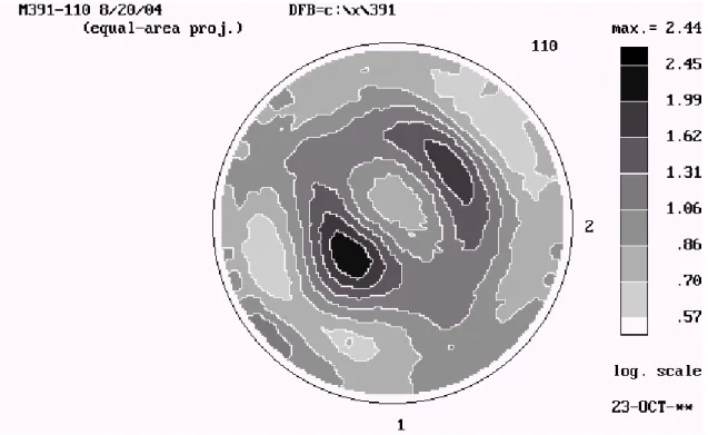
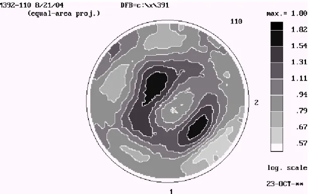
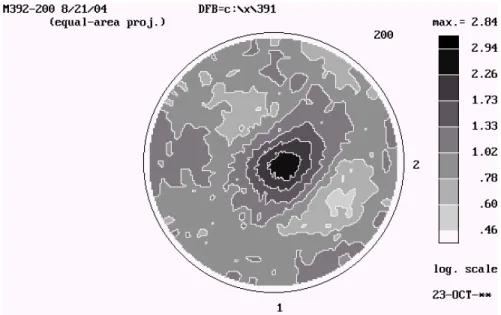
Figure 65: Pole figure for ECAE 4E IF steel (all orientations), direction 3 normal to plane of page ...74

Figure 66: Pole figures for ECAE 8E IF steel (all orientations), direction 3 normal to plane of page...75

Figure 67: Pole figures for ECAE 16E IF steel (all orientations), direction 3 normal to plane of page...75

Figure 68: Inverse pole figures for ECAE 4E IF steel ...76

Figure 71: Low magnification TEM image of as-received IF steel (white bar = 5 μm) ...79

Figure 72: Medium magnification TEM image of as-received IF steel showing dislocations (white bar = 500 nm)...79

Figure 73: Low magnification TEM image of ECAE 1A IF steel (white bar = 2 μm) ...80

Figure 74: Low magnification TEM dark field image of ECAE 1A IF steel (black bar = 1 μm) ...80

(12)

Page Figure 75: TEM dark field image of high dislocation density zones within ECAE

1A IF steel (black bar = 500 nm). Circled region contains “dark

spots”...81 Figure 76: High magnification TEM dark field image of “dark spots” in ECAE

1A ...82 Figure 77: Low magnification TEM image of ECAE 2A IF steel (white bar = 2

μm) ...83 Figure 78: High magnification TEM image of ECAE 2A IF steel (white bar =

200 nm) ...84 Figure 79: Low magnification TEM image of ECAE 2B IF steel (white bar = 2

μm) ...85 Figure 80: High magnification TEM image of ECAE 2B IF steel (white bar =

100 nm) ...86 Figure 81: Low magnification TEM image of ECAE 2C IF steel (white bar = 2

μm) ...87 Figure 82: High magnification TEM image of ECAE 2C IF steel (white bar =

100 nm) ...88 Figure 83: Low magnification TEM image of ECAE 4A IF steel (white bar = 2

μm) ...89 Figure 84: Low magnification TEM image of ECAE 4A IF steel (white bar = 1

(13)

Page Figure 85: Intermediate magnification TEM image of ECAE 4A IF steel (white

bar = 500 nm) ...91 Figure 86: High magnification TEM image of ECAE 4A IF steel (white bar =

200 nm) ...92 Figure 87: Low magnification TEM image of ECAE 4B IF steel (white bar = 2

μm) ...93 Figure 88: Intermediate magnification TEM image of ECAE 4B IF steel (white

bar = 500 nm) ...94 Figure 89: High magnification TEM image of ECAE 4B IF steel (white bar =

100 nm) ...95 Figure 90: Low magnification TEM image of ECAE 4C IF steel (white bar = 1

μm) ...96 Figure 91: High magnification TEM image of ECAE 4C IF steel (white bar =

500 nm) ...97 Figure 92: Low magnification TEM image of ECAE 4E IF steel (white bar = 2

μm) ...98 Figure 93: High magnification TEM image of ECAE 4E IF steel (white bar = 200

nm) ...99 Figure 94: Low magnification TEM image of ECAE 8E IF steel (white bar = 2

(14)

Page Figure 95: Intermediate magnification TEM image of ECAE 8E IF steel (white

bar = 500 nm) ...101 Figure 96: High magnification image of ECAE 8E IF steel (white bar = 200 nm) ...102 Figure 97: Low magnification TEM image of ECAE 16E IF steel (white bar = 2

μm) ...103 Figure 98: Intermediate magnification TEM image of ECAE 16E IF steel (white

bar = 500 nm) ...104 Figure 99: High magnification TEM image of ECAE 16E IF steel (white bar =

200 nm) ...105 Figure 100: 90-minute recrystallization curve for IF steel processed via ECAE

1A ...113 Figure 101: 90-minute recrystallization curve for IF steel processed via ECAE

2B ...114 Figure 103: 90-minute recrystallization curve for IF steel processed via ECAE

2C ...114 Figure 104: 90-minute recrystallization curve for IF steel processed via ECAE

(15)

Page Figure 106: 90-minute recrystallization curve for IF steel processed via ECAE

4C’...116 Figure 108: 90-minute recrystallization curve for IF steel processed via ECAE 4E ...117 Figure 109: 90-minute recrystallization curve for IF steel processed via ECAE

8C’...118 Figure 111: 90-minute recrystallization curve for IF steel processed via ECAE 8E ...118 Figure 112: 90-minute recrystallization curve for IF steel processed via ECAE

16E ...119 Figure 113: Low magnification optical micrograph of as-received IF steel ...122 Figure 114: Optical micograph showing “fiber” structures on as-received IF steel ...122 Figure 115: Microstructures of ECAE 1A IF steel. (a) as-processed, (b) annealed

for 90 minutes at 700°C ...123 Figure 116: Microstructures of ECAE 8C’ IF steel. (a) as-processed, (b) annealed

for 90 minutes at 700°C ...124 Figure 117: Optical micrograph of ECAE 2C IF steel showing worked structure ...125 Figure 118: Optical micrographs of ECAE 1A IF steel. (a) as-processed, (b)

(16)

Page Figure 119: Optical micrographs of ECAE 2A IF steel. (a) as-processed ...127 Figure 120: Optical micrographs of ECAE 4A IF steel. (a) as-processed, (b)

annealed at 550°C...129 Figure 121: Optical micrographs of ECAE 4C’ IF steel. (a) as-processed, (b)

annealed at 550°C...131 Figure 122: Optical micrographs of ECAE 8C’ IF steel. (a) as-processed ...132 Figure 123: Optical micrograph of ECAE 16E IF steel annealed at 700°C for 90

minutes ...134 Figure 124: A “skeleton” image of the grain structure of ECAE 16E IF steel

annealed at 700°C for 90 minutes ...135 Figure 125: Grain size distribution for ECAE 1A IF steel annealed at 700°C for

90 minutes ...136 Figure 126: Grain size distribution for ECAE 2A IF steel annealed at 700°C for

90 minutes ...137 Figure 127: Grain size distribution for ECAE 2B IF steel annealed at 700°C for

90 minutes ...138 Figure 128: Grain size distribution for ECAE 2C IF steel annealed at 700°C for

90 minutes ...139 Figure 129: Grain size distribution for ECAE 4A IF steel annealed at 700°C for

(17)

Page Figure 130: Grain size distribution for ECAE 4B IF steel annealed at 700°C for

90 minutes ...141 Figure 131: Grain size distribution for ECAE 4C’ IF steel annealed at 700°C for

90 minutes ...142 Figure 132: Grain size distribution for ECAE 8C’ IF steel annealed at 700°C for

90 minutes ...143 Figure 133: Grain size distribution for ECAE 16E IF steel annealed at 700°C for

90 minutes ...144 Figure 134: True stress vs. true strain behavior of IF steel after ECAE 1A

processing...154 Figure 135: True stress vs. true strain behavior of IF steel after ECAE 2A

processing...154 Figure 136: True stress vs. true strain behavior of IF steel after ECAE 2B

processing...155 Figure 137: True stress vs. true strain behavior of IF steel after ECAE 2C

processing...155 Figure 138: True stress vs. true strain behavior of IF steel after ECAE 4A

processing...156 Figure 139: True stress vs. true strain behavior of IF steel after ECAE 4B

(18)

Page Figure 140: True stress vs. true strain behavior of IF steel after ECAE 4C

processing...157 Figure 141: True stress vs. true strain behavior of IF steel after ECAE 4C'

processing...157 Figure 142: True stress vs. true strain behavior of IF steel after ECAE 4E

processing...158 Figure 143: True stress vs. true strain behavior of IF steel after ECAE 8C

processing...158 Figure 144: True stress vs. true strain behavior of IF steel after ECAE 8C'

processing...160 Figure 147: Optical micrographs of ECAE 2B IF steel. (a) as-processed, (b)

annealed at 550°C...161 Figure 148: Optical micrographs of ECAE 2C IF steel. (a) as-processed ...162 Figure 149: Optical micrographs of ECAE 4B IF steel. (a) as-processed, (b)

annealed at 550°C...164 Figure 150: Optical micrographs of ECAE 16E IF steel. (a) as-processed...165 Figure 151: Rotation schematic for Route A. PF refers to punch face ...167

(19)

Page Figure 152: Rotation schematic for 90° rotations ...168 Figure 153: Rotation schematic for 270° rotations ...169 Figure 154: Rotation schematic for 180° rotations ...170

(20)

LIST OF TABLES

Page Table 1: Chemical composition of the IF steel used in the present research ...22 Table 2: Processing routes...23 Table 3: Annealing schedule for the ECAE processed IF steel samples...28 Table 4: The composition of the Marshall’s reagent used to reveal grain

boundaries in IF steels...35 Table 5: Summary of tensile test results ...37 Table 6: Vickers hardness measurements taken for the construction of

recrystallization curves...106 Table 7: Temperature ranges of three annealing regimes for the processing routes

(21)

1. INTRODUCTION

Material1 properties are dependent upon material microstructure, crystal structure, and crystallographic texture. Crystallographic texture describes how grains are oriented with respect to a sample coordinate grame. The materials properties and mechanical performance are closely related to its microstructure. Manipulating the microstructure of a material through mechanical deformation, processing, and heat treatment, i.e. thermomechanical treatments, can be used to change material properties.

There are a number of different thermomechanical treatments for changing the microstructure of a material. One commonly used method, rolling, involves reducing one dimension of a materials cross-section by feeding it through a set of rollers. The resulting textures are sometimes called “sheet texture” characterized by a planar structure that runs parallel to the rolling direction. Drawing of a material, in which the material is pulled through a die, can produce wire. The textures associated with drawing are fibrous and are oriented in the direction of drawing. There are many other methods of working a material, including torsion and compression, but one method that is receiving much interest is severe plastic deformation, in particular a special form of extrusion known as equal channel angular extrusion.

The mode of deformation in equal channel angular extrusion (ECAE) is mainly simple shear. This is made possible by subjecting a sample of material, known as a billet, to a high load, forcing the billet through an angled channel. In the case of a

(22)

perfect 90° angled die, it is within this angled channel that the simple shear occurs, causing a change in the materials microstructure across the entire cross-sectional area of the billet. The material that emerges from the process has the same cross-section as the material that entered. This is one of the benefits of the ECAE processing technique. Another benefit offered by ECAE processing is the ability to control the resulting microstructures during subsequent extrusions, by changing the orientation of the billet, rotating it along the long axis.

Post-processing heat treatments permit further modification of the material’s grain structure. Recrystallization within the processed billets relieves some of the internal stresses and restores ductility.

The present research focuses upon the effect of severe plastic deformation strain and path change on the microstructural evolution of a material that has been subjected to equal channel angular extrusion. Multiple extrusion routes and passes through the die were performed, all at a fixed room temperature. Microstructural analysis was conducted to help determine grain size, deformation structure and orientation. The objectives and parameters of this research are: 1) to examine mechanical performance of post-process material through the use of room temperature monotonic tensile tests; 2) determine its hardness using microhardness tests; 3) observe microstructural features through optical microscopy and TEM visualization; 4) examine the texture changes that occur during the processing, both before and after heat treatment, using XRD texture analysis; and 5) examine the recrystallization behavior of the material for different temperatures and a fixed time. The material in question is known as interstitial free (IF)

(23)

steel, a variant of the steel commonly used in the automotive industry for body panels and other “non-exposed” or painted surfaces. To date there have been very few studies of this kind conducted on IF steel at room temperature.

(24)

2. LITERATURE REVIEW

2.1. Properties and Application of Interstitial Free Steel

Interstitial free steel was selected for this study due, in part, to its excellent deep drawing characteristics. Such properties lend this material to wide application in fields ranging from the automobile industry to architectural applications.

As stated previously the automotive industry uses IF steel for body panels and other painted components. Known as “bake hardening” steel, this metal is very easily formed into complex contours using pressing machines. During the forming process dislocations are created within the steel, and are subsequently pinned in place by the few remaining carbon atoms during the paint curing stage of part fabrication. The pinned dislocations make the metal stronger, and the processing stage where this takes place is what gives the metal its name. The use of IF steel in architecture is based upon similar logic: the metal is easily formed into complex shapes. This permits builders to create structures that are more organic in form than previously possible.

2.2. Equal Channel Angular Extrusion

The severe plastic deformation technique known as equal channel angular extrusion (ECAE) was pioneered in Soviet Russia in 1972 by V. M. Segal [1, 2]. This processing technique allows the creation of ultra-fine or nano-scale structures within a material by

(25)

imparting a nearly uniform simple shear load in large billets. Billet dimensions do not change much between the beginning and end of the process (Figure 1). Repetitive extrusions make it possible to control the evolution of the resulting billet microstructure.

The process of ECAE is accomplished by pressing a lubricated billet through two intersecting channels of equivalent cross section. The angle of intersection of these angles may vary, but is typically either 90-degrees or 120-degrees. In the present work the ECAE intersection angle was 90-degrees. Pressing forces and temperature are sometimes varied for research purposes, but for this research the press force was 500,000 pounds, performed at room temperature. Billet lubricant for the ECAE machine used is typically a thin wrapping of Teflon sheet, with the moving parts lubricated by an anti-seize compound that can tolerate high temperatures.

(26)

Figure 2 shows the slip line field and velocity vectors associated with a billet during extrusion. Some assumptions, namely that the billet moves with a constant velocity inside both channels, and that the zone of plasticity is a single β-slip line, lead to some basic operating equations for ECAE. If there is no other force acting upon the transverse plane – that is, the plane that is parallel to the driving punch – then it is possible to calculate the average stress σ along the line OA, as well as the punch pressure p.

θ θ σ cot 2 cot k p k = − =

The variable k in the above equations represents the material shear stress, while θ is the angle between channels.

Figure 2: (a) ECAE slip line diagram; (b) velocity vector diagram [2]

In the event of contact friction between the billet and the die channel walls, the situation becomes a bit more complex. Given a contact friction τ, the slip line field

(27)

becomes more of a fan, and includes a central fan AOB, a zone of rigid metal AO1B, and a zone of uniform stress BOC. These zones are illustrated in Figure 3a and Figure 3b.

Figure 3: (a) Slip line fan with friction forces, (b) velocity diagram [2]

The angle ψ, the fan angle, is calculated using:

(

η θ

)

ψ =2 −

where η=π/2-1/2 Arccos (τ/k) is an angle between slip lines AO and BO. These equations are true when τ>k cos 2θ. With a ratio of length to thickness (L/H), the punch pressure may be calculated as:

(

)

[

]

[

(

)

]

_HL

k

p=2 cot_η+2_η−_θ +_τ sin_η sin_η+cos_η −1 +2τ

Material strain is focused primarily in the fan shape of AOB in Figure 3, and also across the lines AO and BO. The shear within these regions is a simple shear in the direction of the β-slip lines, and may be calculated using:

(28)

[ ]

_η

γβ = =cot

n

v v

After passing through the area AOB the accumulated shear is:

ψ γα = (rad)

with α-slip lines making up the flow lines and indicating the direction of simple shear within the region AOB.

Segal’s work [2] describes the history of a square element within a fictitious billet of material that is undergoing ECAE. The element, confined between flow lines 1-1 and 2-2 (see Figure 4) undergoes repeated stages of simple shear along the line AO, simple shear along the α-slip lines within the AOB region, and simple shear along the slip line BO. The dashed lines and vectors show that the deformation process is not one of a single step of simple shear, but rather a more complex series of different macroslip planes. Full distortion of the element is given by:

η ψ η

ϕ 2cot _sin2

tan = +

This equation, however, does not correspond to simple shear in the flow direction. There are two limiting cases worth noting. First, when η<θ, ψ=0, as shown in Figure 2, and the element distortion and shear strain are given by:

θ ϕ

γ

γ =2 β =tan =2cot

(29)

Figure 4: Deformation history of a square element [2]

In the second case, η=π/2 and distortion is given by:

ψ ϕ γ

γ = α =tan =

These two cases may correspond to situations of both low and high contact friction. Segal’s work uses the axes x, y, z to represent the directions perpendicular to the flow, transverse and longitudinal planes, respectively. The angles associated with these axes, φ1, φ2, and φ3, are the three possible angles of rotation about the flow, transverse and longitudinal axes.

For cases in which φ1= φ2= φ3=0 or when those three angles are divisible by 180°,

the flow is plastic and planar. Structural elements will receive distortion into the plane in these cases. The accumulation of shear may increase continuously, as in the case of Route A (no rotations between extrusions), or alternate between their destruction and

(30)

creation, as in Route C (+180° rotation on even passes, -180° on odd passes). An equation that yields the orientation of any shear plane of Route A at the nth pass out of N

total passes is given by:

(

)

θ

ϕ 2 1 cot

tan _n = N + −n

and is visually represented in Figure 5.

Figure 5: Shear planes of Route A [2]

In the case of Route C, the angle φ2 alternates between ± 180°, causing the shear planes to alternate across the same shear plane. Structural elements are alternatively destroyed and restored between odd and even passes, respectively. Visually, the shear planes of Route C are presented in Figure 6.

Figure 6: Shear planes of Route C [2]

It is possible to rotate the angle φ2 by 90° or even 270°, and these rotations are the basis of Routes B and C’. Routes B and C’ are made up of superpositioning shear

(31)

vectors, as seen in Figure 7. In the case of two rotations of φ2=90°, the first pass performs a simple shear γ1 in the plane yoz, with line 1 indicating the unit element’s

displacement.

Figure 7: The superposition of shear vectors [2]

The second operation induces a second shear, γ2, on the plane xoy, with line 2

indicating the displacement. Adding these vectors gives the equivalent shear:

(

2

)

2 2 1 γ γ γ = +

which lies within plane P, and has a trace O1 O1 at the transverse section zox.

2 1

tan

γγ

(32)

When a billet is alternated between φ2= ±90°, it is following Route B. The billet’s original position is returned after even numbers of passes. The distortion within a billet following Route B is shown in Figure 8 for up to 4 passes in a tool with a die angle of 2θ=90°.

Figure 8: Shear plane orientations within a billet following Route B [2]

For Route C’, the billet is rotated by φ2=+90° after each pass. This has the end effect of returning the billet to its original position after four passes. It should be noted that because subsequent passes are performed upon the previous shear planes, all passes of Route C’ occur on four spatially separate planes. Figure 9 shows the orientation of the shear planes for a billet following Route C’ after four passes through a die angle of 2θ=90°.

(33)

Figure 9: Shear plane orientation within a billet following Route C’ [2]

During multi-pass ECAE, the ends of the billets are subject to “end effects,” which are zones of rigid metal that have not been subjected to the same amount of working as the rest of the billet. Figure 10 (a) and (b) shows process simulations, and Figure 10 (c) and (d) actual billets of aluminum alloy 3003 that have been processed up to Route 4A through a die with an angle of 2θ=90°, the billets having been macroetched to better show the end effects, which vary between route.

(34)

Figure 10: (a) Process simulation of two passes; (b) process simulation of four passes; (c) macroetched Al billet after two passes; (d) macroetched Al billet after four passes [2]

In the case of Route A, the end effect development is fairly easy to visualize and understand. Route C has localized end effects, and there is a periodic repetition of the coordinate grid distortion between odd and even-numbered passes. Route B’s end effects are somewhat similar to Route A’s, except that the areas of non-uniformity are turned on an angle of ω=45° about the y-axis, and are symmetrically arranged on the

(35)

other end of the billet. Route C’ has a more complex distribution of end effects, as after four passes the rigid zones at the billet ends are only partially restored, and are partially distributed across the billet volume.

End effects can impact the amount of fully processed material that a billet can yield, and must be taken into consideration during processing.

When comparing a process such as ECAE to other, more conventional operations, some important differences emerge. Since ECAE is not coupled with a change in geometry there must be some discussion of equivalence. Segal’s work uses equivalence of spent energy through effective stress (σi) and strain (εi). In the case of ECAE simple

shear with no friction, effective stress, strain and punch pressure can be calculated using:

θ θ ε σ cot 2 3 / cot 2 3 k p N k i i = = =

For standard extrusion, the equations for “ideal” forming without friction are:

λ λ ε σ ln 3 ln 3 k p k i i = = =

with λ=Fo/f representing the cross-sectional area reduction from Fo to f. The equivalent

extrusion reduction, based upon the effective strain calculations above, is:

(

2 cot / 3

)

exp _θ

λ_E = N

The equivalent extrusion reduction provides the same spent energy as N passes of ECAE. The ideal conventional extrusion of like final products would require N times higher pressure, and NλE times larger load than the equivalent ECAE process. In the

(36)

event of extremely high values of N, ECAE may be used to achieve very large effective strains under low pressures and loads.

The evolution of texture under ECAE processing was also studied [36]. The researchers observed the evolution of texture in a high purity Al0.5Cu alloy based upon the processing route, the number of passes and the initial texture of the specimen. It was discovered that processing route and number of passes have a very important impact on texture evolution.

Figure 11: Inverse pole figures for Route C’ after two passes for strong (a) and weak (b) initial texture, after four passes for strong (c) and weak (d) initial texture [36]

(37)

Figure 11 shows how the beginning texture impacts the texture results at low numbers of ECAE pass. In the case of Figure 11 (c) and (d), the influence of initial texture begins to decrease. The researchers discovered that, as a general rule, the texture strength shows a decrease as the number of ECAE passes increases. Routes A, B and C’ showed a continuous decrease in texture strength, with Routes A and C’ being most

effective for randomizing the texture after four passes. Given a strong starting texture Route B yields a moderately strong texture after six and even eight passes. Route C exhibits a cyclic evolution in texture strength, with odd-numbered passes showing very weak textures and even numbered passes showing strong textures, as in Figure 12.

(38)

Figure 12: Inverse pole figures of Route C after two (a), three (b), four (c), five (d), six (e) and seven (f) passes [36]

(39)

2.3. The Mechanical Behavior of Metals Subjected to ECAE

When processing metallic materials through a technique such as equal channel angular extrusion, certain changes in mechanical behavior are commonly observed. As ECAE strain levels increase, so too follows the yield stress of the metal [4], while the ductility typically decreases, sometimes significantly [3]. Figure 13 shows the mechanical behavior of 0.15%C steel after having been processed using ECAE.

Figure 13: Tensile properties vs. pass number for ECAE processed 0.15%C steel [19]

The increase in tensile strength is most noticeable at the initial stage of ECAE processing. After the first pass through the die, the increase in both yield strength and ultimate tensile strength decreases. Grain refinement is also most pronounced after the

(40)

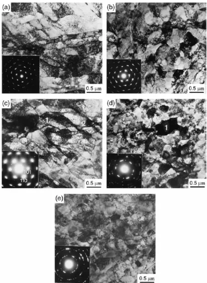
initial stage of ECAE [18], with less significant refinement as the processing is continued, but an increase in high-angle boundaries. Figure 14 shows a series of TEM images of low-carbon steel subjected to increasing passes of ECAE.

Figure 14: Low-carbon steel processed via ECAE Route C: (a) one passes; (b) two passes; (c) two passes, in a different region; (d) four passes; (e) eight passes. Numerals within the figures reference

features relevant to the researcher’s study [18]

To recover some of an as-processed material’s ductility, an annealing heat treatment may be used. During annealing, the sample is placed in a furnace at elevated

(41)

temperatures for an extended period of time, ranging from as little as one hour to as long as 72 hours. At the elevated temperatures of the annealing process, stored internal strain energy from severe plastic deformation is relieved as a result of increased atomic diffusion. Recrystallization, in which new, low strain, equiaxial grains grow, occurs at a certain point during the annealing heat treatment. As recrystallization progresses and crystal grains grow, the mechanical properties associated with the severe plastic deformation revert to a state that is closer to the pre-deformation material; the yield strength and ultimate tensile strength decrease, along with the material’s hardness, while ductility is recovered. Research into the use of annealing after ECAE [4, 7] indicates that samples that are processed using ECAE and then annealed for various lengths of time show superior performance when compared to unprocessed samples. Figure 15 shows this in the case of 0.15 wt.% C steel that has been processed using four passes of Route C.

Figure 15: Stress-strain curves of 0.15C steel, as-received, post ECAE (“As-pressed”), post ECAE (4 passes) and annealed at 753K for 72 hours [7]

(42)

3. EXPERIMENTAL PROCEDURES

3.1. Material

This research was conducted using titanium-stabilized interstitial free steel that was obtained from US Steel Research, Monroeville, Pennsylvania. The chemical composition of this material is shown in Table 1. The raw material used in this research came from US Steel Research in the form of a 21” x 8” x 1” plate. The plate was hot rolled and allowed to slow cool, permitting the IF steel to fully recrystallize.

Table 1: Chemical composition of the IF steel used in the present research

Element Atomic Weight Weight Percent Atomic Percent Fe 55.85 Balance Balance C 12.01 0.0023 0.0107 S 32.07 0.0077 0.0134 N 14.01 0.0018 0.0072 O 16 0.002 0.007 Ti 47.9 0.065 0.0758 Nb 92.91 0 0 Al 26.98 0.05 0.1035 3.2. ECAE Procedures

The billets of IF steel were first rough cut from the bulk plate, and then machined on a mill to the dimensions of 1”x1”x6” in preparation for extrusion. The longitudinal axis of each billet corresponded to the rolling direction. The original plate was hot rolled and allowed to slowly cool and recrystallize, and so was not cold worked. The texture of the

(43)

as-received material indicated a strong texture in the [111] and [001] directions of the transverse plane of the billets. All billets were extruded at room temperature at a rate of 0.1 inch per second, using a variety of routes and passes. Table 2 shows the routes and number of passes used in this study. Graphical representations of the billet rotations for each route are provided in the Appendix.

Table 2: Processing routes

Sample Group Number Extrusion Route 0 / As-Received No Extrusions Performed 1 Route 1A 2 Route 2A 3 Route 2B 4 Route 2C 5 Route 4A 6 Route 4B 7 Route 4C’ 8 Route 4C 9 Route 4E 10 Route 8C’ 11 Route 8C 12 Route 8E 13 Route 16E

Prior to extrusion, anti-seize lubrication was applied to both the billet and the moving surfaces of the extrusion machine in an effort to reduce the friction during the extrusion process. IF steel is easily extruded at room temperature with a punch speed of 0.1 inches per second.

(44)

The formation of flash was a common side-effect of the extrusion process because of the wearing of the tool over time. Flash occurred along most corners of the billet, and at the point of contact between the punch and the billet. The flash was easily removed using a high speed rotary grinder. The extrusion process caused some dimensional changes from the norm as a result of friction and tool wear, and these were addressed using a combination of rolling (performed on the flow faces) and milling (performed on the longitudinal faces) to make the billet ready for further processing. Recrystallization does not occur until approximately 500°C in IF steels, so the process of machining a billet was not expected to cause a significant recovery or recrystallization.

3.3. Tension Testing

Tension testing was performed to examine the mechanical behavior of ECAE processed IF steel. Tension tests were conducted on specimens that were both as-processed and post-process annealed, to examine the impact of recrystallization on mechanical response. The tension tests in this study were conducted until failure occurred. To obtain the tension test specimens, cubes of approximately 1” x 1” x 1” were first cut from processed billets on a diamond saw, and the tension sample profiles were cut using wire EDM. The tension sample profile is shown in Figure 16. Once the bulk tension profile was cut, the individual specimens were sliced from the bulk profile, again using wire EDM. Every tension specimen was cut such that the profile face corresponded to the flow plane of the billet and load direction was parallel to the extrusion direction. The thickness of each tension specimen was two millimeters, with

(45)

the exception of the tension specimens from Routes 4A and 4B, which were cut to 1.5 mm thickness. 3.00 mm 9.00 mm 8.00 mm R2.00 mm 7.00 mm 7.00 mm 3.50 mm 3.50 mm DIA 1.56 mm 2X DRILL THROUGH

Figure 16: Schematic of the tension sample profile

The samples were all coated with a thin film of residue that is normal for EDM processing. This thin film was removed by hand-sanding each specimen first with a

(46)

600-grit pad, and then finished off with an 800-grit pad. The objective was to remove any surface imperfections that could interfere with the extensometer during tension testing and cause stress concentration areas.

Tension testing was performed on an MTS brand machine with a computer recording the output data. Simple experiments were conducted to check the modulus of the samples before each tension test to verify measurement accuracy. The strain rate was 0.004 sec-1 for all experiments. The data collected from the test series was then evaluated using programs such as Microsoft Excel and Igor Pro. Of particular interest were the shape of the complete stress-strain response, the yield and ultimate tensile strengths, and the ductility at failure of each specimen. To check for repeatability, two or three companion specimens from each case were tested.

The annealed tension specimens were tested and evaluated in the same manner as the as-processed specimens. A light hand-sanding of each specimen was performed prior to the tension tests so as to remove any residue that may have collected during the annealing heat treatment. Of particular interest was how the annealing process influenced the ductility of the material, or the level of strain on a material just prior to failure.

3.4. TEM

The transmission electron microscopy done in this research was conducted at the University of Paderborn, Germany. IF steel was processed into foils for use in the TEM system. First, a slice of about 1 mm to 1.5 mm thickness was cut from the original

(47)

sample. This slice was then polished using SiC paper to a grit of 4000, and then finished with twin-jet electropolishing.

Transmission electron microscopes resolve images by emitting a beam of electrons through a specially prepared specimen. Internal microstructural details are resolved, and contrasts in the image are produced by beam scattering and diffraction off of the microstructure or defect. Solid materials are very absorptive to electron beams, so the specimen being imaged must be a very thin foil. Once the beam penetrates through the specimen, it is projected onto a fluorescent screen or photographic film for viewing [39].

3.5. Heat Treatment and Construction of Recrystallization Curves

A diamond saw was used to cut out sections of ECAE-processed billets for use in constructing recrystallization curves. The cuts were done such that the largest surface was that of the flow plane. In order to construct these curves each sample was annealed for 90 minutes at temperatures ranging from 100°C to 700°C, then mounted into epoxy, ground to a surface finish of 800-grit, and finally tested for hardness. Heat treatments were performed in air inside a Lindberg/Blue brand box furnace, followed by quenching in water at the end of annealing. The schedule for the heat treatments conducted in this study is shown in Table 3.

(48)

Table 3: Annealing schedule for the ECAE processed IF steel samples Annealing Temperature (°C) Annealing Time (minutes)

100 200 300 350 400 450 500 550 600 700 90

For each temperature, ten microhardness measurements were taken on each sample. All results will be presented in the experimental results section.

3.6. Texture

All texture measurements were performed at the University of Paderborn, Germany. The planes under examination are identified as 1, 2, 3, and correspond to the flow plane, longitudinal plane, and transverse plane, respectively.

Obtaining a pole figure requires the use of X-ray diffraction systems. X-ray diffraction systems make use of alignment characteristics of the crystal lattice in regards to the reflection of incident rays of radiation with varying wavelength off of crystallographic surfaces. Using the Bragg law, which governs how waves of radiation are diffracted from the parallel atomic planes of crystals, it is possible to generate a map of the arrangement of crystals within a specimen. In equation form, the Bragg law appears as

(49)

θ

λ 2dsin

n =

where n is an integer, λ is the wavelength (in nanometers), d is the interplanar distance

within the crystal, and θ is the angle of incidence or reflection of the radiation.

X-ray diffractometers use devices such as Geiger countertubes or ionization chambers instead of photographic plates to detect the reflected radiation from a sample [32]. These machines, at the basic level, consist of a source of parallel X-rays, a rotating sample holder that is held at an angle of incidence θ to the X-ray source, and a Geiger countertube that is held at an angle 2θ from the incident X-rays. Both the sample holder and the Geiger countertube rotate, with the Geiger counter tube always rotating at twice the speed of the specimen holder. This doubling of speed is necessary if the Geiger countertube is to remain in position for receiving the reflected radiation from the specimen.

(50)

Figure 17: Schematic of an X-ray diffractometer [40]

In Figure 17, T represents the target emitting X-rays, B and C are slits and collimator assemblies, S is the specimen holder, D is the X-ray detector, and G is a goniometer scale graduated in degrees.

3.7. Hardness Measurements

One method of determining the recrystallization temperature is to measure the change in hardness of a specimen. There is a significant drop in hardness due to softening of the material during recovery and recrystallization. Hardness, or the resistance of a material to penetration or indentation, is determined by applying a constant force on the material’s surface via an indenter. For the hardness measurements in this study, Vickers microhardness was measured. Vickers hardness makes use of a square shaped diamond indenter, which leaves a pyramidal indentation in the surface of

(51)

the sample. The diagonal dimensions of this pyramid indentation are measured, and from that the hardness value is calculated. Vickers hardness, or HV, is the ratio of applied load to the surface area of the indentation left on the sample’s surface.

The hardness testing machine used in this research was a Buehler Micromet II Digital Micro Hardness Tester. A load of 1000 grams (g) was applied for a duration of 15 seconds. Such test conditions permitted a well-defined indentation to form, allowing more accurate readings. It is important to have a smooth, flat surface on the specimen, in order to better identify the contours of the indentation. Every sample used in this research was given an initial rough grinding on 240-grit paper, and then transferred in groups of six samples to the automatic grinding machine for further grinding with 400-grit, ending with 800-grit paper. The samples were then rinsed with water, followed by alcohol, and then dried under a heated blower. All hardness measurements were performed on the flow plane for each route studied. When performing the hardness measurements, the recommended spacing between adjacent indentations was at least three times the average indentation diameter. The rationale behind this spacing is that for each load applied to the surface, there may be a zone around the indentation where material stresses have increased; therefore, each indentation must be made outside of this zone of stress. In measuring the recrystallization curves, ten measurements were recorded for each specimen. The highest and lowest microhardness values were ignored in order to obtain a better calculation of the average hardness.

(52)

3.8. Metallography

To examine the microstructure of the specimens using optical metallography, the specimens were subjected to the following processes: sectioning, mounting, polishing and etching. These processes are described in the following paragraphs.

Cutting specimens out of the as-processed billets is an important step, and should therefore be done with care and attention to detail. If done properly, a good sectioning will not interfere with hardness measurements. Carelessness can lead to improper mechanical loading, which could damage the diamond blade, introduce mechanical hardening, or cause localized annealing due to heat buildup. Standard cutting techniques tend to introduce an inclination of the specimen, leading to misorientation of the desired surface. To maintain as precise an orientation as possible, the sections were cut using a Buehler Isomet 1000 diamond saw, which was cooled with an oil-water lubricant to keep cutting temperatures low.

All specimens were mounted in Buehler Epoxicure epoxy. Epoxy mounting was used first because of its low curing temperature, and second because it cures clear, making it possible to insert identifying labels into each specimen for quick reference.

The grinding of the specimens was performed via the traditional method of abrasive removal of material from the surface. Typically this is accomplished through the use of a grinding wheel with an attached grinding pad. This wheel rotates at a set rate, and the sample is pressed against the grinding pad, initiating the surface grinding. To improve the surface finish of the specimen, successive grinding stages make use of smaller abrasive particle sizes. Once a small enough particulate size is reached, the process

(53)

becomes known as polishing, and makes use of liquid abrasive solutions and polishing pads. The stages of grinding and polishing are performed in order to prepare the specimen’s surface for microstructural evaluation and hardness testing. It is important to obtain as smooth a surface as possible, since scratches may negatively impact the results of optical microscopy. The use of automated grinding and polishing machines has made this stage of sample preparation more efficient, since multiple samples can be ground and polished at the same time.

All of the specimens used in this phase of the research were given an initial rough grinding treatment by hand. This was performed on a Buehler Ecomet 3 machine, using rough 240-grit grinding disks. First a chamfer with an angle of approximately 45° was ground into the epoxy in order to reduce grinding friction during the later stages of surface preparation. Next the sample was subjected to a rough grinding to remove any thin film of epoxy that might exist on the surface of the sample. Once the rough grinding was completed, the samples were gathered into groups of six for further surface preparation using a Buehler automatic grinding machine. The automatic grinding machine allowed adjustments in grinding time, downward force during grinding, and direction of circular rotation during the grinding cycle. For the purposes of this research, the grinding time was kept as 10 minutes, the downward force was 24 pounds, and the platter rotated in a counter-clockwise direction. Initial grinding on the automatic grinding machine was performed with disks of 400-grit surfaces, then finished with 800-grit disks. Upon completion of the final grinding step, the platter was removed from the power head and rinsed under running water, sprayed with alcohol to prevent watermark

(54)

formation, and dried under a heater. The resulting surface finish was acceptable for microhardness testing of the various samples.

To obtain a good optical image, the surface finish must be of high enough quality to reflect back large amounts of light. Good results in microscopy also require a flat, scratch free surface finish on the sample in question. Using the correct polishing surface and abrasive compound, it is possible to obtain a mirror-like surface finish on a specimen. Unlike grinding, where the abrasive is bonded onto the surface of the grinding disk, the abrasive particles used in polishing are so small they must be held in a suspension, typically in the form of liquid slurry or as a paste that is then applied to a soft polishing wheel.

For IF steel, a regimen of progressively finer grit polishing compounds is applied to clean polishing cloths. The polishing begins with an initial surface grind at 240-300 rpm, under moderate pressure, using 320-grit SiC paper for one minute. The next phase, lasting five minutes and rotated opposite the direction of the polishing wheel, is performed at 120-150 rpm, with moderate pressure, using 9-μm diamond paste applied to an Ultra-Pol cloth, and Metadi Fluid as a lubricant. After cleaning the specimens, a four minute polish at 120-150 rpm, using 3-μm diamond paste and Metadi Fluid lubricant on a Trident cloth is performed. A similar polish using 1-μm diamond paste is recommended for materials such as IF steel. The final polishing stage is performed for 2-3 minutes using 0.05-μm Masterprep Alumina slurry on a wet MicroCloth polishing cloth.

(55)

It is important to maintain a high level of cleanliness during the polishing stage. Routine distilled water rinses are used during the polishing stage, sometimes followed up with ultrasonic cleaning if there are any pockets of foreign material trapped between the specimen and the epoxy. A thorough rinse with alcohol prevents any staining during the drying stage.

Before any etching was performed, the specimens were examined under an optical microscope. This preliminary examination was done to identify any defects, such as pores, pits, inclusions or scratches, which could result in a possible adverse reaction during etching.

Even after polishing is complete, the final surface of the IF steel samples will not have any visible microstructure under optical microscopy. This is because the incoming light is uniformly reflected. To expose grain boundaries and produce contrast between grains a chemical etch is employed. Since IF steel has such a low carbon content, conventional etchants such as Nital can not be used. Instead a mixture of Marshall’s reagent and hydrofluoric acid is used. The composition of the Marshall’s reagent is presented in Table 4.

(56)

The recommended mixture of Marshall’s reagent to hydrofluoric acid is 100:1 ml, with the etching performed through immersion of the sample. Marshall’s reagent works well for exposing the grain structure of low carbon steels, such as IF steel.

(57)

4. EXPERIMENTAL RESULTS AND DISCUSSION

4.1. Tensile Testing

Tensile testing is a standard method of examining the mechanical behavior of materials. Of interest in this study were the value of ECAE-processed IF steel’s yield strength, ultimate tensile strength, and ductility. The description of the tensile testing performed in this study was presented in Section 3.3. A summary of the values of yield strength, ultimate tensile strength and ductility for each sample used in the as-processed tests is shown in Table 5. The values are presented as true-stress for YS and UTS, and engineering-strain for % ductility. Engineering-strain was chosen because the equations for converting to true-stress and true-strain do not apply after plastic deformation begins.

Table 5: Summary of tensile test results

Sample YS (MPa, true) UTS (MPa, true) Ductility at Failure (%, Engineering)

As Received 70.7 282.3 60.3 1A 442.7 467.8 29.3 2A 496.3 526.3 10.7 2B 532 571.2 45.2 2C 522.7 561.6 45.6 4A 593.1 636.3 27.1 4B 590.9 634.8 18.8 4C' 602 678.2 41.5 4C 552.7 588.3 16 4E 555.5 651.2 41.7 8C' 681.2 776.3 43.4 8C 575.4 634.6 41.9 8E 613.2 704.7 39.6 16E 654.2 758.9 44.7

(58)

A comparison of these values makes it possible to see, at a glance, the impact ECAE has on the mechanical performance of IF steel (Figure 18). Yield strength shows a dramatic improvement at the first pass through the press. In the case of Route A, there is a steady increase in the yield strength as the number of passes increases. The same increase is observed in Route B, although the increase is not as noticeable. In the case of Route C the increase in yield strength is very slight, especially between ECAE 4C and ECAE 8C. For Route C’ the increase in yield strength is more noticeable; ECAE 8C’ has the highest yield strength of all of the processing routes used in this study. Route E shows some degree of yield strength enhancement, though it is not as great as Route C’.

0 100 200 300 400 500 600 700 800 As Re ceiv ed 1A 2A 2B 2C 4A 4B 4C' 4C 4E 8C' 8C 8E ₁₆E Yield St ren g th , MPa

(59)

In Figure 19 a comparison of tensile strength across the various routes is made. Route A shows a steady increase in the value of UTS from ECAE 1A to ECAE 4A. Route B shows a less significant increase in comparison to Route A. The increase in ultimate tensile strength in Route C as the number of passes increase is very slight. Route C’ shows a significant increase in ultimate tensile strength, and again ECAE 8C’ has the highest recorded values for ultimate tensile strength. Route E shows a steady increase in its UTS values, with ECAE 16E having the second-highest ultimate tensile strength recorded.

The ductility of the IF steel tension test samples is presented in Figure 20 so as to allow a comparison between the routes that were examined in this study. Comparisons of ductility at failure across the different routes show unusual results. In the case of Route A, the first specimens showed a decrease from ECAE 1A to ECAE 2A, and then an increase to ECAE 4A. Route C showed a similar behavior. The ductility of Route B decreased as the number of passes increased. The opposite is true for Routes C’ and E:

(60)

0 100 200 300 400 500 600 700 800 900 As R ecei ved 1A 2A 2B 2C 4A 4B 4C' 4C 4E 8C' 8C 8E ₁₆E U ltim a te Te n s ile S tr e ngth, M P a

Figure 19: A comparison of ultimate tensile strength of as-processed IF steel

0.0 10.0 20.0 30.0 40.0 50.0 60.0 70.0 As R eceiv ed 1A 2A 2B 2C 4A 4B 4C' 4C 4E 8C' 8C 8E _16E D u ctili ty a t Fail ure (% , E ngin eer ing S tr a in)

(61)

The summaries that were presented in Figures 18 – 20 present only the yield strength, ultimate tensile strength and ductility values of the specimens tested. They do not show the actual true-stress versus true-strain curves obtained from the test data. The ductility data presented in Figure 20 is taken from engineering strain values. Plots of the true-stress versus true-strain performance of the different routes examined in this study are presented in Figures 21 – 25 on the following pages. In each case the as-received material true-stress versus true-strain curves are shown for comparison purposes. Because the values for true-stress and true-strain were obtained using the equations

(

)

(

engineering

)

true g engineerin g engineerin true ε ε ε σ σ + = + = 1 ln 1

the strain values after the ultimate tensile strength should not be considered accurate by the reader.

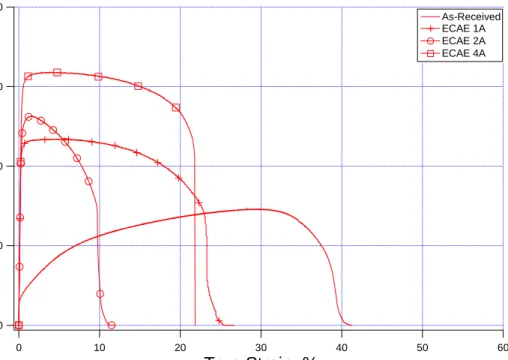
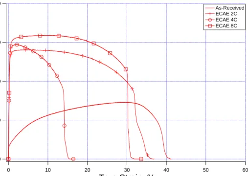
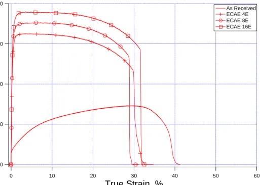
True-stress versus true-strain behavior for specimens processed using Route A is shown in Figure 21. True-stress versus true-strain behavior for specimens processed using Route B is shown in Figure 22. True-stress versus true-strain behavior for specimens processed using Route C is shown in Figure 23. True-stress versus true-strain behavior for specimens processed using Route C’ is shown in Figure 24. True-stress versus true-strain behavior for specimens processed using Route E is shown in Figure 25.

(62)

800 600 400 200 0 Tr ue St re ss , MPa 60 50 40 30 20 10 0 True Strain, % As-Received ECAE 1A ECAE 2A ECAE 4A

Figure 21: True-stress vs. true-strain comparison of IF steel processed using Route A

800 600 400 200 0 Tr ue St re ss , MPa 60 50 40 30 20 10 0 True Strain, % As-Received ECAE 2B ECAE 4B

(63)

800 600 400 200 0 Tr ue St re ss , MPa 60 50 40 30 20 10 0 True Strain, % As-Received ECAE 2C ECAE 4C ECAE 8C

Figure 23: True-stress vs. true-strain comparison of IF steel processed using Route C

800 600 400 200 0 Tr ue St es s, MPa 60 50 40 30 20 10 0 True Strain, % As Received ECAE 4C' ECAE 8C'

Figure 24: True-stress vs. true-strain comparison of IF steel processed using Route C’

(64)

800 600 400 200 0 Tr ue St re ss , MPa 60 50 40 30 20 10 0 True Strain, % As Received ECAE 4E ECAE 8E ECAE 16E

Figure 25: True-stress vs. true-strain comparison of IF steel processed using Route E

The data plots shown in Figures 21 – 25 are useful for examining how the mechanical properties of as-processed IF steel change as the number of passes increase in a given route. A comparison of the routes, given a constant number of passes, allows an examination of the impact routes have upon mechanical performance. In all cases, the true-stress vs. true-strain behavior of the as-received material is included for reference purposes.

The plot comparing routes given two passes (Figure 26) shows that ECAE 2A yields poor YS and UTS when compared to ECAE 2B and ECAE 2C. In the cases of ECAE 2B and ECAE 2C, their YS is virtually identical, and their UTS values are also quite similar.

(65)

When four passes are considered (Figure 27), there are more routes available for examination: ECAE 4A, ECAE 4B, ECAE 4C, ECAE 4C’ and ECAE 4E. Of these, ECAE 4C’ and ECAE 4E show the highest values of YS and UTS.

In the case of eight passes (Figure 28), there are three routes that can be compared: ECAE 8C, ECAE 8C’ and ECAE 8E. It is shown that the mechanical performance of ECAE 8C’ is superior to the other routes in this instance. The UTS of ECAE 8C’ is the highest recorded in this study.

800 600 400 200 0 Tr ue St re ss , MPa 60 50 40 30 20 10 0 True Strain, % As Received ECAE 2A ECAE 2B ECAE 2C

Figure 26: Comparison of routes at two passes for as-processed IF steel

(66)

800 600 400 200 0 Tr ue St re ss , MPa 60 50 40 30 20 10 0 True Strain, % As-received ECAE 4A ECAE 4B ECAE 4C ECAE 4C' ECAE 4E

Figure 27: Comparison of routes at four passes for as-processed IF steel

800 600 400 200 0 Tr ue St re ss , MPa 60 50 40 30 20 10 0 True Strain, % As-received ECAE 8C ECAE 8C' ECAE 8E

Figure 28: Comparison of routes at eight passes for as-processed IF steel

(67)

To examine the impact of annealing on as-processed IF steel, tension specimens from three ECAE processing routes were annealed and tested. The annealing temperatures chosen corresponded to those of the early and middle stages in recrystallization, between 400°C and 600°C, with annealing times ranging from five to 90 minutes. In the case of ECAE 4A, three samples were annealed; one at 500°C for five minutes, one at 600°C for five minutes and the last at 600°C for 15 minutes. In the case of ECAE 4E, two specimens were annealed for 90 minutes each, one at 450°C and the other at 500°C. In the case of ECAE 8E, three specimens were annealed for 90 minutes each, one at 400°C, another at 500°C and the last at 600°C.

True-stress vs. true-strain plots from these annealed specimens are shown in Figures 29 – 31.

The plot for ECAE 4A (Figure 29) shows that a short anneal of 15 minutes at 600°C significantly reduces both YS and UTS values. The true-stress vs. true-strain curve for ECAE 4A that has been annealed at 500°C for five minutes shows inferior values of YS and UTS. When annealed for 600°C for five minutes, the true-stress vs. true-strain plot shows a decrease in YS and UTS in comparison to the as-processed sample. The YS and UTS of the sample annealed for five minutes at 600°C is lower than those values for the sample annealed at 500°C for the same time.

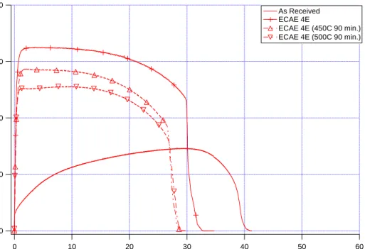
In the case of ECAE 4E the true-stress vs. true-strain plots of Figure 30 show a steady decrease in YS and UTS as the 90-minute annealing temperature increases.

The true-stress vs. true-strain results for ECAE 8E are shown in Figure 31. All of the tension specimens were annealed for 90 minutes in this case. When annealed at

(68)

400°C the YS is slightly lower than the as-processed material, but the UTS values are both lower than the as-processed curves. At 500°C the sample displays a YS lower than that of the 400°C sample, with a UTS that is almost identical to the YS. At the highest annealing temperature, 600°C, the true-stress vs. true-strain curve shows similar behavior to the as-received curve. At 600°C the ECAE 8E tension specimen displays somewhat improved YS and UTS, in comparison to the as-received sample.

800 600 400 200 0 Tr ue S tr e ss , M P a 60 50 40 30 20 10 0 True Strain, % As Received ECAE 4A ECAE 4A (500C 5 min.) ECAE 4A (600C 5 min.) ECAE 4A (600C 15 min.)

(69)

800 600 400 200 0 Tr ue St re ss , MPa 60 50 40 30 20 10 0 True Strain, % As Received ECAE 4E ECAE 4E (450C 90 min.) ECAE 4E (500C 90 min.)

Figure 30: True-stress vs. true-strain behavior of as-processed and annealed ECAE 4E IF steel

800 600 400 200 0 Tr ue St re ss , MPa 60 50 40 30 20 10 0 True Strain, % ECAE 8E ECAE 8E (400C 90 min.) ECAE 8E (500C 90 min.) ECAE 8E (600C 90 min.) As Received

Figure 31: True-stress vs. true-strain behavior of as-processed and annealed ECAE 8E IF steel

(70)

4.2. Hardness

Vickers hardness measurements are taken for two reasons: first, to determine how different ECAE processing routes impacts the mechanical behavior of IF steel; second, to identify the temperature at which recrystallization occurs within the processed billets.

4.3. Texture

The objective of the texture analysis was to examine how different processing routes of ECAE impacted the preferred grain orientation in IF steel, and whether this preferred grain orientation might be responsible for some of the anisotropy we observe in mechanical properties.

Pole figures and inverse pole figures are standard methods of visualizing textures. Inverse pole figures may be used to locate certain billet planes, such as the longitudinal, flow and transverse planes, with respect to the poles [001], [101], and [111]. All pole figures are oriented with the flow plane (1) normal to the bottom, the longitudinal plane (2) normal to the right, and the transverse plane (3) normal to the center. In Figure 32 these orientations are depicted in relation to a billet.