The clustering and evolution of massive galaxies

(1)

Durham E-Theses

Ross, Nicholas Patrick

How to cite:

Ross, Nicholas Patrick (2007) The clustering and evolution of massive galaxies, Durham theses, Durham University. Available at Durham E-Theses Online: http://etheses.dur.ac.uk/2523/

Use policy

The full-text may be used and/or reproduced, and given to third parties in any format or medium, without prior permission or charge, for personal research or study, educational, or not-for-prot purposes provided that:

• a full bibliographic reference is made to the original source • alinkis made to the metadata record in Durham E-Theses

• the full-text is not changed in any way

The full-text must not be sold in any format or medium without the formal permission of the copyright holders. Please consult thefull Durham E-Theses policyfor further details.

Academic Support Oce, Durham University, University Oce, Old Elvet, Durham DH1 3HP e-mail: [email protected] Tel: +44 0191 334 6107

(2)

The copyright of this thesis rests with the author or the university to which it was submitted. No quotation from it or information derived from it ma; be published without the prior written con~nt of the author or university, and any mformation derived from it should be acknowledged.

THE

CLUSTERING AND EVOLUTION

OF MASSIVE GALAXIES

NICHOLAS PATRICK ROSS

--

,rDurhalll

University

A thesis submitted to the University of Durham in accordance with the regulations for admission to the

Degree of Doctor of Philosophy.

The copyright of this thesis rests with the author. No quotation from it should be published without their prior

written consent and information derived from it should be acknowledged.

UNIVERSITY OF DURHAM

2007

(3)

THE CLUSTERING AND EVOLUTION OF MASSIVE GALAXIES NICHOLAS PATRICK ROSS

ABSTRACT

In this thesis we investigate the clustering and evolutionary properties of massive galaxies. We present new measurements of galaxy clustering over a range of redshifts using data from the 2SLAQ Survey and the AAOmega LRG Pilot Survey. The clustering properties of Luminous Red Galaxies (LRGs) are measured using nearly 9 000 2SLAQ LRGs at a mean redshift of

z = 0.55. We find that the real-space 2-point correlation function is well described by a single power-law of the form ~(r)

=

(r/ro)--r, where 'Y

=

1.72 ± 0.06 and the correlation length ro = 7.45 ± 0.35 h-1 _{Mpc. Then we study the redshift-space distortions that are present} in the clustering signal. From these dynamical and geometric distortions, we derive a value of Dm

=

0.30 ± 0.15 and {3(z

=

0.55)

=

0.45

±

0.05, where Dm is the present day matter density parameter and {3 = Dm/b where b is the linear bias parameter. We find for 2SLAQ LRGs, b(z

= 0.55)

= 1.66 ± 0.35.

If one then assumes a "high-peaks" bias model, this value of b is consistent with the measured clustering strengths for low-redshift, massive early-type galaxies, under the assumption that gravitational growth leaves the comoving space density of early-types independent of redshift. We then use the new AAOmega instrument to perform a study of redshift z ,..., 0.7 LRGs selected using riz-band photometry. We find a redshift-space correlation length of so

=

9.9

± 0.5

h-1 Mpc and show that using LRGs as tracers would be a very competitive strategy for baryon acoustic oscillation studies in future galaxy redshift surveys. We also confirm that this population again has a clustering strength consistent with the above "high-peaks" bias model. Finally, we use data from the Spitzer and Hubble Space Telescopes taken in the COSMOS field and find tentative evidence for dust emission possibly coming from obscured star formation. We also show that

z ,...,

0.7 LRGs are predominantly early-type galaxies.

(4)

List of Figures

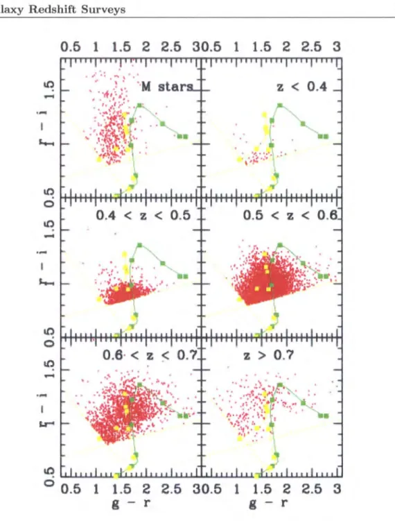
2.1 The SDSS ugriz-bands . . . . 2.2 2SLAQ LRG selection boundaries in the gri two-colour plane

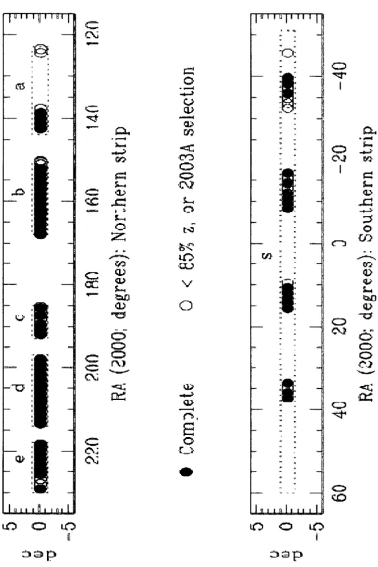
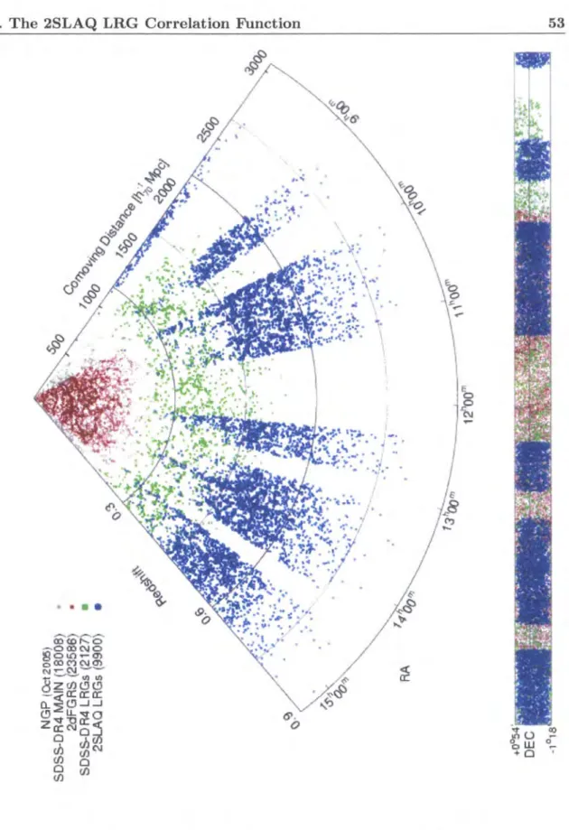
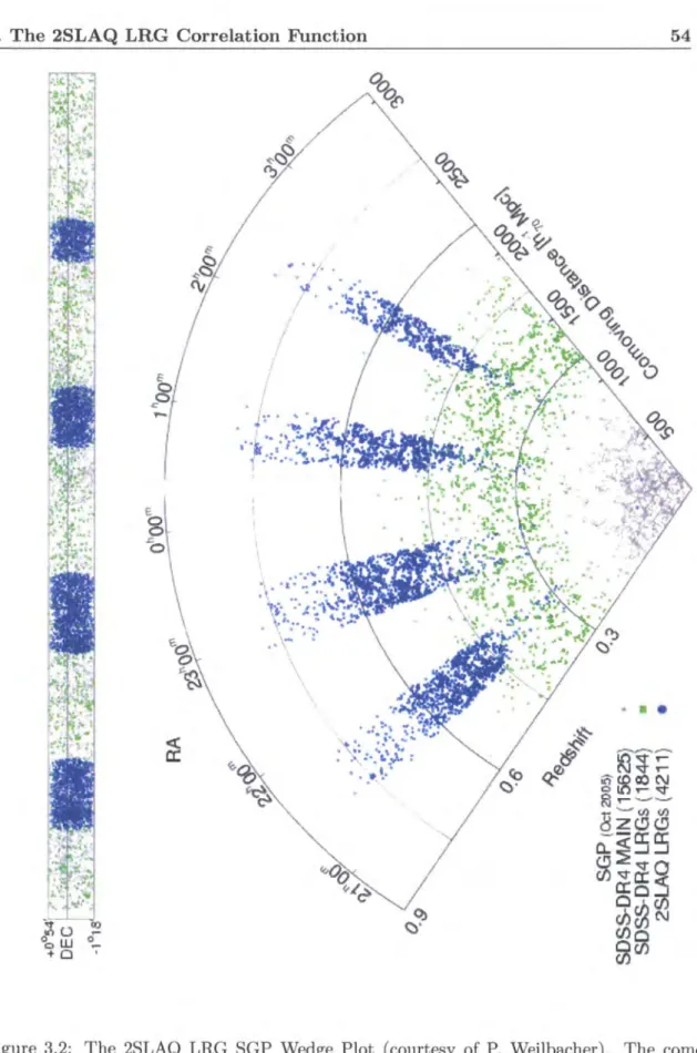
2.3 The redshift distribution in the gri-plane for confirmed 2SLAQ objects . 2.4 The location of the 2SLAQ Input Catalogue and Observed fields . . . . 3.1 The distribution of 2SLAQ LRGs from the Final 3 Year catalogue towards the

28 39 40 44

North Galactic Pole . . . 53 3.2 The distribution of 2SLAQ LRGs from the Final 3 Year catalogue towards the

South Galactic Pole . . . 54 3.3 The angular correlation function, w(O), for the 2SLAQ LRG Input and Redshift

catalogue . . . . 3.4 The redshift distribution for the 2SLAQ LRG "Gold" Sample 3.5 The error ratio for Poisson, Field-to-field and jackknife errors

3.6 The angular correlation function, w(O), from the 2SLAQ LRG Survey

3.7 The redshift-space 2-point correlation function, e(s), for the 2SLAQ LRG Survey 59 62 65 72

in a A and f!m

= 1 Cosmology . . . 73

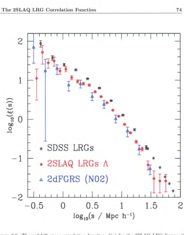
3.8 The redshift-space 2-point correlation function, e(s), for the 2SLAQ LRG Survey,

the SDSS LRG Survey and the high luminosity early-type 2dFGRS . . . 74

(7)

LIST OF FIGURES V 3.9 The de-projected correlation function, wp((J), for the 2SLAQ LRG Survey, the

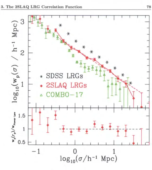
SDSS LRG Survey and the COMB0-17 Red Sequence . . . 78 3.10 The real-space 2-point correlation function, ~(r), for the 2SLAQ LRG Survey for

the A cosmology. . . 81 3.11 The c5x2 _{likelihoods from the joint 2 parameter fits on}

ro

_{and 1}_for_~(r). ₈₄ 4.1 The ~((J, 1r) contour plot for the 2SLAQ LRG Survey, assuming ACDM . 88 4.2 The ~((J, 1r) contour plot for the 2SLAQ LRG Survey, assuming Om = 1.0 89 4.3 Likelihood contours of 0~-,B(z

= 0.55), assuming a A cosmology . . . . .

99 4.4 Likelihood contours of 0~-,B(z

= 0.55), assuming an

Om

= 1.0 cosmology

. 100 4.5 Joint likelihood contours of 0~-,B(z = 0.55) using the geometric method of the

Alcock-Paczynski test, modelling the redshift-space distortions and including the evolution of clustering constraints, assuming the A cosmology . . . 103 4.6 Joint likelihood contours of 0~-,B(z

=

0.55) using the geometric method of the

Alcock-Paczynski test, modelling the redshift-space distortions and including the evolution of clustering constraints, assuming an Om = 1.0 cosmology. . 104 4.7 ~(s)/~(r) for the 2SLAQ LRG Survey . . . 106 5.1 The selection of z"' 0.7 LRGs using the SDSS riz-bands . . 118 5.2 The N(z) of the AAOmega LRG Pilot . . . 122 5.3 Star-Galaxy Separation using SDSS z-band magnitudes . 123 5.4 COMB0-17 photometric redshifts vs. AAOmega spectroscopic redshifts. . . 125 6.1 The AAOmega LRG Pilot angular correlation function, w(O) . . . . . 128 6.2 The AAOmega LRG Pilot De-projected Correlation Function, wp((J) . 133 6.3 The AAOmega LRG Pilot Redshift-Space Correlation Function, ~(s) . 135

(8)

LIST OF FIGURES vi

7.1 The COSMOS field at 3.6JLm . . . 153

7.2 A zoom in on the COSMOS field, showing the large structure at redshift z ~ 0.73 at 3.6JLm . . . . 154 7.3 SDSS i-band- 3.6JL colours for AAOmega COSMOS LRGs as a function of redshift161

7.4 3.6JLm-4.5 JLm Near Infrared colours for AAOmega COSMOS LRGs as a function

of redshift . . . 162

7.5 3.6JLm-8.0 JLm Near Infrared colours for AAOmega COSMOS LRGs as a function

of redshift . . . . 7.6 r- z-3.6JLm colour-colour plane for AAOmega COSMOS LRGs. 7.7 Morphologies of the AAOmega COSMOS LRGs . . . . 7.8 r- z-3.6JLm for AAOmega COSMOS LRGs with morphologies

. 163 . 165 . 167 . 169 7.9 3.6JLm- 8.0 JLm near Infrared colours as a function of redshift with morphologies 171 7.10 r-i-z plot with a selection of AAOmega COSMOS LRGs and their morphologies

with redshifts . . . 172 7.11 A selection of AAOmega COSMOS LRGs with regular, early-type morphologies

with varying redshifts . . . 17 4 7.12 A selection of AAOmega COSMOS LRGs with interesting morphologies . 175

(9)

List of Tables

1.1 The current best estimates of certain cosmological parameters . . . 22 2.1 A comparison between the 2dFGRS, SDSS LRG and 2SLAQ LRG Surveys 35 2.2 Values for Bruzual and Chariot stellar population synthesis models used in gri

colour-colour plots . . . 37 3.1 The 2SLAQ LRG Survey; Numbers of galaxies in different samples . . . 55 3.2 The 2SLAQ LRG Survey; Names and Right Ascension ranges for the N

=

9

sections used when calculating the field-to-field errors. . . . , . . . 66 3.3 Values of the redshift-space correlation length and slope for the 2SLAQ LRG

Survey from

e (

s). . . 76 3.4 Values of the projected correlation function, wp(O"), correlation length and slope

for the 2SLAQ LRG Survey. . . 79 3.5 Values of the correlation length and slope for the 2SLAQ LRG Survey from the

real-space correlation function,

e (

r). . . . 82 4.1 Best fitting model values of Om, (3 and pairwise velocity dispersion, (w;)1₁_{2 ,}_using

redshift-space distortions alone and assuming a A cosmology. The third column gives the range of pair separations used in the fit. . . 97 5.1 Details of the 3 AAOmega LRG Pilot fields . . . 113

(10)

LIST OF TABLES viii 5.2 Redshift Statistics for the AAOmega LRG Pilot Run .

5.3 LRG percentage redshift completeness rates . . . .

6.1 Values of

so

and

ro

from the VST-AAn ATLAS LRG Pilot, SDSS LRG Survey . 117 . 119

and the 2SLAQ LRG Survey. . . 134 6.2 A comparison between the effective volumes probed by LRGs vs. ELGs . 139 7.1 A list of Spitzer names, acronyms and abbreviations . 148

7.2 Spitzer IRAC details . . . . . 148

7.3 The Spitzer COSMOS IRAC fields . 151

7.4 The AUTOPHOTOMIP/OP file format . 157

(11)

DECLARATION

The work described in this thesis was undertaken between October 2003 and April 2007 whilst the author was a research student under the supervision of Prof. Tom Shanks in the Department of Physics at the University of Durham. This work has not been submitted for any other degree at this, or any other, university.

The major collaborators involved in this thesis are Prof. Tom Shanks, Dr. Jose da Angela and Dr. Phil Outram. Minor collaborators include Dr. David Wake and Dr. Alastair Edge, with Prof. John Peacock contributing Section 6.2.2.

Results from this thesis have appeared in the following papers:

• Ross, N.P. et al., submitted to MNRAS, astro-ph/0612400 (Chapters 3 and 4) • Ross, N.P. et al., submitted to MNRAS, astro-ph/0704.3739 (Chapters 5 and 6) and • Cannon, R.D., et al., 2006, MNRAS, 372, 425, (astro-ph/0607631), which provides the

source for a significant part of Chapter 2. However, since the thesis author was an integral member of the 2SLAQ Survey team (spending 12 nights observing at the Anglo-Australian Telescope), a co-author on this paper and the relevant details are vital to this thesis, we reproduced parts of this paper herein. All graphs are either originally produced or reproduced by the author, except where explicitly stated.

Results from this thesis have also appeared in the following conference proceedings:

• Ross N.P. & Shanks, T. 2006, ASP Conf. Proc., Vol. 379

(12)

CHAPTER

1

INTRODUCTION

His name was Gaal Dornick and he was just a country boy who had never seen Trantor before. That is, not in real life. He had seen it many times on the hyper-video, and occasionally in tremendous three-dimensional newscasts covering an Imperial Coronation or the opening of a Galactic Council. Even though he had lived all his life on the world of Synnax, which circled a star at the edges of the Blue Drift, he was not cut off from civilization, you see. At that time, no place in the Galaxy was.

- Isaac Asimov, Foundation.

1.1

MODERN COSMOLOGY

The current Big Bang Theory is based on three pillars of observation:

1. The expansion of the Universe.

2. The Cosmic Microwave Background.

3. Nucleosynthesis of light elements.

The first of these comes from observing distant galaxies and noting that the Doppler shift of the spectral lines implies these galaxies are receding in all directions. We shall return to the expansion of the Universe in due course.

(13)

1. Introduction 2 Observations of the Cosmic Microwave Background (CMB), have come to maturity in the last 15 or so years. The power spectrum of the temperature anisotropies that are measured in the CMB tell us a wealth of information about the content of the Universe. The latest results are presented below (Section 1.1.3).

The third of these pillars does not directly concern us here and the reader is directed to reviews such as Boesgaard & Steigman (1985) and Buries et al. (1999) for further details and discussion.

1.1.1 THE HUBBLE EXPANSION

Although scientists prior to Edwin Hubble had suggested it, e.g. Curtis (1920) and references therein, it was Hubble who first presented evidence for the velocity-distance relationship of galaxies (Hubble, 1929),

v =Hod ( 1.1)

where v is recessional velocity in units of kilometres per second (kms-1 ), d is distance from observer in units of megaparsecs (Mpc) and Ho is the present-day value of a constant of pro-portionality, now called Bubble's Constant where we define h

=

Ho/100 km s-1 Mpc-1 to parameterise our ignorance of the exact value of Ho. The estimate of the velocity at which an object is receding, is made from the spectrum of the emitted light,

(1.2)

where Aobs is the observed wavelength of a photon, A lab is the wavelength of the photon measured in a laboratory and z is the redshift.

(14)

1. Introduction 3

1.1.2 GRAVITY, MATTER AND GEOMETRY

The timing of Rubble's observations were critical. Ever since Albert Einstein had formulated his General theory of Relativity in 1916 (GR; Einstein, 1916), various attempts had been made to solve the GR Field equations and build a cosmological model.

Alexander Friedman (or Friedmann) in 1922, Georges Lemaitre in 1927 and Roward Robert-son and Arthur Walker in 1933 all investigated the most general homogeneous, isotropic and non-stationary solutions for the field equations of GR. As such, we can write down the Friedmann-Lemai'tre-Robertson-Walker (FLRW) metric which is an exact solution of the Einstein field equations of GR. This describes a homogeneous, isotropic expanding or contracting universe,

(1.3)

where

t

is the time coordinate and the spatial coordinates are represented in polar form. The constant k represents the spatial curvature, of the Universe. a(t) is the scale factor, which represents the time dependence of cosmological distance due to the expansion of the Universe and is related to the redshift by ao/ a = 1

+

z where the index 0 indicates the present time and a(to) = ao = 1.

This metric gives rise to the Friedmann Equation, which relates the evolution of the scale factor to the overall energy density of the Universe, p,

(1.4)

where G is the gravitational constant and H(t) gives the rate of expansion of the Universe and is called the Rubble Parameter, with H(t = to) = Ho. The energy-density and pressure of the fluids of the Universe are related via the Fluid Equation,

(15)

1. Introduction 4 and combining Equations 1.4 and 1.5 gives rise to the Second Friedmann equation which de-scribes the Universe's acceleration,

~

= _

47rG (P

+

3p) .

a 3 c2 (1.6)

Here we can decompose the general energy-density term, p into three parts,

P =PM+ P-y

+

PA, (1.7)

where M stands for the matter content of the Universe, 'Y for the radiation content of the Universe and A for the contribution of the vacuum energy-density. We can also write down an Equation of State which relates the density and the pressure of the fluids we are considering,

(1.8)

where w is the equation of state parameter and c is the speed of light, which will be omitted from here on. Since p

=

wp, then w

=

pj p and it follows from equations 1.4 and 1.5 (or equation 1.6) that p ex a-3_(1+w). _{For non-relativistic matter,}_PM ₌ _{0 implying}_w ₌ _{0 and}

p ex a-3. For radiation, p-y

=

p/3 implying w

=

1/3 and p ex a-4. At early times, when a was small, radiation played the dominant role in the expansion. However, today, the radiation content of the Universe seems to have a negligible contribution to the energy budget (Mather et al., 1990). For our purposes, we can therefore assume P-y = 0 from here on. For the vacuum: PA

= -pA sow= -1 and p ex

a0. This value of w

= -1 is what is required for a "Cosmological

Constant". This was a term first introduced by Einstein into the GR field equations when he was trying to reconcile a theoretically dynamic system with the contemporary observational evidence of a static Universe. Note that any equation of of state with w

< -1/3 implies that

the rate of the Hubble expansion is increasing.

(16)

1. Introduction

Using Equation 1.4, we can define a critical density,

with k

=

0 and n _ Pt ~G- ' Pc

PA

OA=-. Pc 5 (1.9) (1.10) If 0 = 1, the Universe is said to be "flat" and the energy-density is equal to the critical density. Recent measurements from e.g. distant Type la Supernovae (SNe I; Riess et al., 1998, 2004, 2006; Perlmutter et al., 1999), large-scale structure (LSS; Eisenstein et al., 2005; Cole et al., 2005; Tegmark et al., 2006; Percival et al., 2006a) and the CMB (Spergel et al., 2003, 2006), suggest that this is indeed the case and the Universe is (or is very near to) flat. These recent measurements also suggest that nM

<

1 and thus for a flat Universe where nM

+

nA = 1, OA

# 0. The best current values for these O's are given below in Section 1.5.2.

1.1.3 THE COSMIC MICROWAVE BACKGROUND

The FLRW Universe and the idea of an early very hot and very dense universe was fully confirmed by the detection of the CMB in 1965 by Penzias and Wilson (Penzias & Wilson, 1965) along with the theoretical interpretation by Dicke, Peebles, Roll and Wilkinson (Dicke et al., 1965).

The original detection of the CMB by Penzias and Wilson has been followed by many other experiments and missions, all of them too numerous to mention here. However, three of the most critical missions have been on board the COBE satellite, the BOOMERanG balloon and the WMAP satellite. COBE (COsmic Background Explorer; Smoot et al., 1992) showed that the CMB was extremely well represented by black body emission with a temperature of 2. 73 K, while there were also tiny, 1 part in 105 , temperature anisotropies.

(17)

1. Introduction 6 The BOOMERanG (Balloon Observations Of Millimetric Extragalactic Radiation and Geo-physics; de Bernardis et al., 2000; Netterfield et al., 2002) was the first experiment to make a significantly large area, high signal-to-noise observation of the CMB temperature anisotropies, such that when combined with a contemporary value of

Ho,

gave strong indications that the Universe had a flat geometry, at least under certain assumptions of the matter components.

The Wilkinson Microwave Anisotropy Probe ( WMAP; Bennett et al., 2003) satellite had the main aim to measure the temperature anisotropies in the CMB. With the publication of the 3 year WMAP data (Jarosik et al., 2006) the angular power spectrum of temperature anisotropies is known to exquisite accuracy (Hinshaw et al., 2006) and the polarisation power spectrum has also been measured (Page et al., 2006). WMAP has provided an exquisite measurement of the acoustic peaks in the temperature anisotropy power spectrum, placing strong constraints on certain cosmological parameters.

The almost completely homogeneous nature of the CMB on large scales, combined with the ax-iom that we do not live in a special region of the Universe, leads to the Cosmological Principle:

There is no preferred location or direction in the Universe; the Universe is homogeneous and isotropic

(18)

1. Introduction 7

1.2

STRUCTURE FORMATION

1.2.1 DENSITY FLUCTUATIONS

On the largest scales the Universe is believed to be homogeneous and isotropic. However, the primordial density fluctuations first detected in the CMB radiation by COBE, correspond to fluctuations in the matter density and it is the subsequent growth of these matter density fluctuations that give rise to the stars, galaxies and superclusters we see today. These tiny matter fluctuations of size 8 are described by

8(x) = p(x)_-ji = 8p

P

PO

(1.11)

where p(x) is the local density and p = Po is the mean density of the Universe. We can then define the auto-correlation function as

~(r) = (8(x)8(x

+

r)) (1.12)

where r =

lrl

is a measurement of the separation between two local overdensities. 8(x) can also be written as a sum of its Fourier modes,

8(x) =

L

8k exp(ik · x)

=

L

8Z exp( -ik · x). (1.13)

k k

with the power spectrum, P(k), being defined as

(1.14) where k is the wavenumber, and the scale (or wavelength) ..\ of a fluctuation is related to the wavenumber k by k = 211' / ..\. If the primordial density fluctuations are drawn from a Gaussian distribution, the power spectrum gives a complete statistical description of the fluctuations. One could assume, in its simplest form, the power spectrum could be a power law,

(19)

1. Introduction 8 where the index, n, governs the balance between large and small scale power. A power spectrum with n = 1 will have no preferential scale and is called a Harrison-Zeldovich spectrum. The Harrison-Zeldovich spectrum is often the choice for a primordial Power Spectrum, Ppri(k), where the primordial Power Spectrum at very high redshift is related to the Power Spectrum observed at recombination by

(1.16)

Here, T(k) is the transfer function and conveys all the information about the pre-recombination evolution and the nature of the matter content. Indeed, the transfer function will give a pre-scription for the weak oscillatory features that are expected, given the Universe has a non-zero baryon content. These are called the baryon acoustic oscillations (BA Os). Also, as the density contrast grows and 8pj p becomes

>

1, non-linear evolution will contribute signatures in the density field.

The relationship between the power spectrum, P(k), and the correlation function, ~(r), is given by

(1.17)

In an isotropic universe, the density perturbation cannot contain a preferred direction, and so we must have an isotropic power spectrum: (18ki2_(k))₌

i8ki

2_(k). _{Also, if}_J.L_{is the cosine of the}

angle between k and r, then noting that ~ is real, the integral over all directions of r gives

(1.18)

and therefore,

(1.19)

(20)

1. Introduction 9 from "'0.1 to"' 20 h-1 Mpc, the correlation function, (, is well described by a power-law such that

((r) =

(;o)

-~

(1.20)

where r0 is the correlation length and 1 is the power-law slope with ro ~ 5 h-1 Mpc and 1 ~ 1.8 in the range 0.1 h-1 Mpc ::;; r ::;; 10 h-1 Mpc (e.g. Shanks et al., 1989).

1.2.2

EVOLUTION OF STRUCTURE

If one probes large-enough scales such that non-linear effects are not relevant, then the growth of density perturbations is given by (e.g. Peacock, 1999)

(1.21)

where c8

= Jopjop is the sound speed. To simplify matters, we can ignore the second term in

the brackets (originating from the consideration of pressure gradients) and also assume nM

= 1

and 47rGp0 = 3H2 /2

==

2/3t2. Then we have two solutions,

o(t) <X t213 or

c

1. (1.22)

Let us consider the first solution, the "growing mode", where 8 p / p <X t213• As a marker, opj p"' 1/1

+

z in a baryonic, nM = 1 Universe. As first seen by COBE, oT /T "' 2 x

w-

5 on 1 o scales and thus opj p"' 6 x

w-

5 at a redshift of z"' 1100. Today at redshift z = 0, we predict opj p"' 6 x

w-

2

• Essentially, this is not a large enough density contrast to explain the large-scale structure we observe at the present epoch in the universe. Very small fluctuations in the CMB, growing only by gravity, form the inhomogeneous structures of galaxies, groups and clusters we observe today. It is therefore one of the key tasks of modern cosmology to understand the other components of the Universe such that the large observed density contrasts can be explained.

(21)

1. Introduction 10 One of these additional components is cold dark matter (CDM) which is suspected to be a massive yet collisionless form of matter and which does not emit electromagnetic radiation, hence the description 'dark'. The 'cold' refers to the non-relativistic motions of the theorised dark matter particles.

By combining equation 1.21 with equation 1.4 we can probe the evolution of the density perturbations in different cosmological scenarios. We can then measure the clustering of struc-ture and compare with that from linear theory and N-body predictions, in order to determine the density parameters that describe the energy content of the Universe.

1.2.3 FURTHER INGREDIENTS FOR LARGE-SCALE STRUCTURE

Before we can give a final recipe for large-scale structure we must introduce one more assump-tion.

This assumption is that the luminous matter in the Universe traces the overall underlying matter distribution. With good evidence that galaxies more massive than the smallest dwarfs are unable to prevent luminous star formation e.g. Taylor & Webster (2005) (however see also Minchin et al., 2005), it seems reasonable that the luminous matter distribution will in some way trace the underlying matter distribution. However, it is also reasonable to assume that the luminous matter might be a biased tracer of the overall matter distribution. As an initial guide, we can define the linear bias parameter, b, as

(1.23)

where 8g is the galaxy density contrast and DM the mass density contrast. Further care has to be taken when discussing bias since we know (e.g. Saunders et al., 1992; Norberg et al., 2002a) that different populations have different measured biases values and indeed bias may be

(22)

1. Introduction 11 scale-dependent (Smith et al., 2007, and references therein). The investigation of bias will be one of the main themes in the remainder of this thesis.

Now we can give the ingredients for large-scale structure; a primordial n = 1 Harrison-Zeldovich Power Spectrum; T(k) the transfer function (including the weak oscillatory features that are expected if the Universe has a non-zero baryon content); non-linear clustering; cold dark matter and a bias prescription will together all lead to suggestions of what one might see in a galaxy clustering observation.

One of the best ways to study the clustering and evolution of large-scale structure is by performing surveys of the cosmic web. By statistically analysing the clustering of galaxies from redshift surveys, we can probe how structure has grown and study the evolutionary properties of the Universe as it expands.

(23)

1. Introduction 12

1.3

GALAXY REDSHIFT SURVEYS

Over recent years the results from two redshift surveys have dramatically increased our under-standing of large-scale structure and the extra-galactic population locally. The 2 degree Field Galaxy Redshift Survey (2dFGRS; Colless et al., 2001, 2003) used the 3.9m Anglo-Australian Telescope (AAT) and the 2dF instrument with its multi-fibre optics to observe and measure red-shifts for rv220,000 galaxies over 1 700 square degrees of the Southern Hemisphere. The 2dFGRS probed galaxies with luminosities ranging from 0.1£ * ;S L ;S 2L * and redshifts of 0

<

z

<

0.3*. The primary science aims that the 2dFGRS achieved included measuring the power spectrum and detection ofbaryon acoustic oscillations (Percival et al., 2001; Cole et al., 2005), both optical (Norberg et al., 2002b) and near-infrared luminosity functions (Cole et al., 2001), measurement of the cosmological mass density via clustering (Peacock et al., 2001; Hawkins et al., 2003) and the investigation of various galaxy properties by galaxy type (e.g. Madgwick et al., 2003). An incomplete list of further discoveries included obtaining an upper limit on the total neutrino mass (Elgar0y et al., 2002), studying the biasing properties of galaxies (Verde et al., 2002; Wild et al., 2005) and examining galaxy groups (e.g Eke et al., 2004). Observations were completed in 2002 and the full 2dFG RS catalogue can be found at http: I /www. mso. anu. edu. au/2dFGRS/.

The Sloan Digital Sky Survey (SDSS; York et al., 2000) combines a five-band imaging survey of the northern Galactic Cap, with a multi-fibre spectroscopic follow-up programme. The observations for the primary SDSS have been completed, and the final data release, DR5 was made in July 2006. The DR5 Imaging footprint is 8 000 square degrees, and the number of unique objects in the Imaging Catalogue is 215 million, while the Spectroscopic footprint was 5 740 square degrees, and the number of spectra in the Spectroscopic Catalogue is 1 048 960.

(24)

1. Introduction 13 The SDSS collaboration plan to have three further data releases (DR6 through DR8) as part of the "SDSS-II" project.

The SDSS spectroscopic survey consists of two parts. The dominant portion, with about 88% of the fibre allocation, was a flux-limited sample that reached a magnitude of r = 17.77 (Strauss et al., 2002). This is commonly referred to as the MAIN sample.

The other 12% of the galaxy spectroscopic sample was devoted to galaxies fainter than the MAIN galaxy flux cut but which were expected, based on observed colours, to be intrinsically red and at higher redshift. This is the more specialised redshift survey, called the SDSS Luminous Red Galaxy (LRG) Survey. At the outset, the goal of the SDSS Luminous Red Galaxy sample was to produce a volume-limited sample of intrinsically luminous (~ 3L*) red galaxies out to

z = 0.5 (Eisenstein et al., 2001). The mean redshift of the SDSS LRG Survey is z ~ 0.35 (e.g. Tegmark et al., 2006).

1.3.1 Luminous Red Galaxies

The primary science driver for the SDSS LRG spectroscopic survey was to probe a volume of "" 1h-3 _Gpc3 _{with sufficient galaxy number density to yield a definitive detection of the BAO} signature in the clustering signal. Luminous Red Galaxies are the ideal candidate galaxies to use for this task for several reasons. They are intrinsically luminous and therefore visible to large distances. They also have distinctive colours leading to a clean and efficient selection. However, the primary reason for choosing LRGs was that they have the ideal number density for probing the Power Spectrum around the BAO scale of k ,...,_ 0.05 h Mpc-1_. _{The amount of cosmological} information gleaned from a galaxy redshift survey depends on the "effective volume" that is surveyed, where effective volume is given by (e.g. Tegmark, 1997; Sea & Eisenstein, 2003;

(25)

1. Introduction 14 Eisenstein et al., 2005; Tegmark et al., 2006)

V:

=

j [

n(r) P(k) ] 2 d3

elf 1

+

n(r) P(k) r (1.24)

where n(r) is the comoving number density of the sample, in units of h3 Mpc-3, and P(k) is the value of the Power Spectrum at wavenumber k.

Ve!f

has units of volume, h-3 _Mpc3

. A commonly used expression for the error on the Power Spectrum measurement is from Feldman et al. (1994),

Cfp

E(

1)

- -

1 +

-p nmodes nP

(1.25)

where nmodes is the number of Fourier modes present in spherical shell, width 8k, which depends upon the survey volume, V: nmodes

= 47r

28k/(27r)3. The first term on the right hand side of this equation can be thought of as the sample variance, while the second term on the RHS can be thought of as the Poisson shot noise term. Using values quoted in Eisenstein et al. (2005), LRGs having n"'

w-

4 _h3 _Mpc-3 _{and P(k}_~_0.05)₌_{4 x 10}4_h-3 _Mpc3 _{thus leads to a value of} nP"' a few, which reduces the shot noise term.

The final reason for choosing LRGs is that they are the most massive galaxies and are believed to reside in over-dense peaks of the underlying matter distribution and are thus po-tentially excellent tracers of large scale-structure. Put another way, they are highly biased objects. The linear bias parameter, b, relates the power spectrum, or correlation function, of the luminous tracers (i.e. galaxies) to that of the underlying matter distribution via

(1.26)

or equivalently

(26)

1. Introduction 15 This relates to equation 1.25, and essentially means that fewer galaxies are required to make the same accuracy of measurement if they have larger biases. As a guide, an ,..., L * galaxy from the 2dFGRS has ab ~ 1 (Norberg et al., 2002a), while a ,..., 3L* SDSS LRG has b ~ 2 (Padmanabhan et al., 2006).

The SDSS LRG Survey has achieved its main aim in regarding the detection of BAOs e.g. Eisenstein et al. (2003, 2005); Tegmark et al. (2006); Percival et al. (2006a,b). This detection is strong experimental evidence that we now have a detection and measurement of the Doppler Peaks in the local, z

«

1, Universe, connecting them to the those at the last scattering surface at z,..., 1100. However, BAOs are not the only dynamical and geometric information contained in the clustering signal.

(27)

1. Introduction 16

1.4

REDSHIFT-SPACE DISTORTIONS

Measuring the clustering of distant objects in redshift surveys does not provide a direct deter-mination of their true spatial distribution, or the real-space clustering of the underlying dark matter. The "real-space" distances are distorted by dynamical distortions due to peculiar ve-locities and also by geometric distortions if the wrong cosmology is assumed when converting the observed redshifts into physical distances. Thus, the distances estimated from an objects' redshift, will not correspond to a true distance and are therefore said to have been measured in redshift-space ( z-space).

1.4.1 DYNAMIC DISTORTIONS

When a redshift is measured, the assumption is made that there are two terms contributing to the galaxy's motion. The first (and usually dominant term) is from the Rubble Expansion, VH, while the second term is due to the contribution from the objects' own peculiar motion, Vpec· This peculiar velocity term itself contains two contributions, due to two mechanisms involved in the redshift-space dynamical distortions.

The first part of the peculiar velocity from the mndom motion a galaxy has due to the influence of its local potential well. If the distribution of distant galaxies has, on average, a spherically symmetric clustering pattern in real space, then a large velocity dispersion- caused by random motions - will cause the clustering signal at small scales to be smeared along the line-of-sight. These features are often referred to as "Fingers-of-God" and can be seen in radial wedge plots of distant galaxy surveys.

The second part of the peculiar velocity is due to coherent infall. As structures in the Universe grow through gravity, the flow and infall of objects from low density to higher-density

(28)

1. Introduction 17 regions contributes to the measured redshifts. At larger-scales this leads to a "flattening" of the clustering signal along the line-of-sight. The infall can be parameterised by comparing the large-scale clustering in real- and redshift-space. In terms of the power-spectrum, Kaiser (1987) showed

(1.28) where the subscripts r and s refer to the real- and redshift-space measurements respectively.

JL is the cosine of the angle between the wavevector k and the line-of-sight. /3 relates the observed large-scale infall to the clustering of the underlying matter and is defined below. For completeness, we can also note at this point that Pgal(ks) can be decomposed (Cole et al., 1994),

Pgal(ks) Pgal(kr)(1

+

/3JL2)2

= _{[ ( 1}

+

~/3

+

~/3

2

)

_Po(JL)

+

( 4 _3/3

+

_7{34

2)

_P2(JL)

+

( :

5{3

2)

P4(JL)] Pgal(kr) (1.29) where the Pt(JL) are the Legendre polynomials with Po

=

1, _P2

=

(3JL2 - 1)/2 and P4

=

(35JL4 - 30JL2 - 3)/8. Equation 1.28 above can be written in terms of the correlation function as well (Hamilton, 1992),

(1.30)

{3 is related to cosmology and the matter distribution by {3 "'- J(O~, n~, z)

- b (1.31)

where the 0 superscripts imply present day values of Om and OA, and b is the linear bias (men-tioned above in equations 1.23, 1.26 and 1.27), which relates the luminous matter clustering

(29)

1. Introduction 18 to that of the underlying matter. f(D~, n~, z) quantifies the growth of structure as a function of the cosmological parameters (Peebles, 1980),

which in the case of a flat Universe can be approximated to (Lahav et al., 1991),

where the second term is usually neglected. Hence,

{3(z) = Dm(z)0.6 b

(1.32)

(1.33)

(1.34)

Landy & Szalay (2002) point out there are currently four different frameworks regarding the estimation of {3 that have been developed; 1) by measuring the ratio of the z and real-space correlation function/power spectrum (e.g. Loveday et al., 1996; Hawkins et al., 2003); 2) by measuring the ratio of the quadrupole to monopole moments of the z-space correlation func-tionjpower spectrum (e.g. Hamilton, 1993; Cole et al., 1994; Peacock et al., 2001); 3) by setting the amplitude of the modes of the redshift-space galaxy density field, {3 and the power spectrum as model parameters (Heavens & Taylor, 1995; Ballinger et al., 1995) and 4) the method given in Landy & Szalay (2002) itself, estimating {3 by Fourier inverting the z-space distortions seen in the density field.

1.4.2 GEOMETRIC DISTORTIONS

The second type of distortions that can affect clustering measurements and lead to anisotropies in the clustering signal are due to geometric distortions.

The conversion between redshift,

z,

and distance,

r,

in a fiat (Dm

+

nA

= 1) Universe, with a cosmological constant is (e.g. Peebles, 1993);

(30)

1. Introduction 19

r - _5_

r

--;===d=z='====

- Ho Jo

Jn?n(l

+

z')3

+

0~

(1.35)

Here, r is the line-of-sight comoving distance. However, as shown by Alcock & Paczynski (1979), if one assumes a cosmology that is different from the true, underlying cosmology of the Universe to convert redshifts to distances, the effect on separations along the line-of-sight, differs from the effect across the line-of-sight. As a consequence, the clustering signal might appear elongated (or squashed) in the redshift direction. As shown by those authors, these geometric distortions can be a powerful cosmological test, namely to determine OA. If D.z is the redshift difference between two galaxies, and D.O their angular separation then,

D.z zD.O

DA(z)(1

+

z) czjH(z)

where H(z) is the Rubble Parameter at redshift z and

(1.36)

(1.37)

is the angular diameter distance (assuming a spatially flat universe with matter and cosmological constant). This ratio is close to unity for small

z,

but at high redshift, it deviates from unity, by an amount that depends on the cosmological parameters.

As discussed in Ballinger et al. (1996), it is however non-trivial to disentangle the effects of geometric distortions from those caused by peculiar velocities. As we shall see later, while there is a degeneracy in the effects seen by both dynamical and geometric distortions, if you can correctly take into account the dynamical signature in a galaxy clustering measurement, one then has a road into making a measurement of the value of OA.

(31)

1. Introduction 20

1.5

THE CURRENT PARADIGM

1.5.1 THE BARYON ACOUSTIC OSCILLATIONS

The initial prediction of the acoustic phenomenon in the early universe was made by Peebles & Yu (1970) and Sunyaev & Zeldovich (1970).

The early universe at ~ 400, 000 years after the Big Bang, consisted of a plasma of mainly electrons, protons, and CMB photons which is usually referred to as the photon-baryon plasma. The fluid is self-gravitating, leading to the growth of over- (and under-) densities as the plasma collapses in localised regions. However, radiation pressure acts as a repulsive, restoring force and thus oscillations akin to sound waves are set up. The resulting acoustic peaks are seen in the CMB angular power spectrum (de Bernardis et al., 2000; Netterfield et al., 2002; Spergel et al., 2003, 2006).

At redshift of z ~ 1100 when the Universe cools sufficiently to allow hydrogen atoms to form, the epoch of Recombination, the photon-baryon plasma decouples and the sound waves are frozen into the matter distribution. A preferential scale, s, is then set such that

{tRee

s

=

Jo

dt C8(t) (1

+

ZRec) (1.38) which gives a zeroth-order estimate for the physical value of the preferential scale. If, tRee

=

379 000 yrs, c8 = cf

J3

and ZRec = 1089 then s ~ 70 h-1 M pc ~ 100 M pc.

In the local redshift z ~ 0 Universe, this preferential scale can be detected in the underlying matter distribution traced out by the luminous matter, i.e. by galaxies.

The power of the BAO signature comes by realising that BAOs can be used as a standard ruler at different cosmological epochs. Thus by measuring the scale of acoustic oscillations at

(32)

1. Introduction 21 the galaxy power spectrum (or correlation function) one can use this standard measuring rod to see if the geometry of the Universe has changed due to the effects of an accelerated cosmological expansion.

We have already noted the need for redshift surveys of the cosmic web as a prime investi-gatory tool into the clustering properties of galaxies and the evolution of large scale structure. We now note, the need for redshift surveys that sample large volumes of the Universe in order to detect the faint BAO signature at rv 100 Mpc scales.

1.5.2 THE FASHIONABLE COSMOLOGY

The current values of certain cosmological parameters derived from large-scale structure and CMB measurements are presented in Table 1.5.2. These values are from the "Vanilla" model quoted in Tegmark et al. (2006, Table Ill, 3rd column;) and from the "b6" parameter model in Sanchez et al. (2006, Table 3, 3rd column). Care should be made when comparing these values of cosmological parameters in Table 1.5.2 since different assumptions and prior information are used for both. However, for the values quoted above, the joint-constraint estimates are used and we can see that all the values quoted are consistent. Note that in both cases the value of Ototal is set to 1 and w, the equation of state parameter for vacuum energy, is fixed at -1. From these values we see that baryonic matter is only ~ 4% of the energy-density content and contributes "' 18% of the total matter content. The other 82% or so of the matter content is classed as dark matter i.e. ndark matter ~ 0.196 Ototal· Meanwhile, it seems that more than ~ of the Universe's energy-density is in the form of

nA -

popularly called dark energy.

Thus, since we have no direct confirmation of a dark matter sub-atomic particle, and if the values in Table 1.5.2 are correct, we are left in a slightly embarrassing- but extremely exciting

(33)

Parameter Tegmark et al. (2006) Sanchez et al. (2006) h 0 730+0.022 _. _-0.018 0 735+0.022 _. _-0.018 Ototal 1 1 nA 0 761+0.017 _. _-0.018 0 763+0.020 _. _-0.020 Omatter 0 239+0.018 _. _-0.017 0 237+0.020 _. _-0.020 nbaryon 0 042+0.002 . -0.002 0 042+0.002 . -0.002 WA -1 -1

Table 1.1: The current best estimations of certain Cosmological Parameters from Tegmark et al. (2006) and Sanchez et al. (2006). A flat cosmology is assumed in both cases and hence OtotaJ=l. Note also that in both cases, the value of w, the equation of state parameter is fixed to -1 and the mass of neutrinos is also set to M11 = 0.

(34)

1. Introduction 23 - position of not knowing what 95% of the Universe is made of. The nature of the "Dark Sector" is arguably the most challenging problem not only in astrophysics but in the whole of the physical sciences at the beginning of the 21st Century. As such we need as many different routes and examples of independent proof to actually verify the claim that dark energy and dark matter actually exist.

(35)

1.6

MOTIVATION AND LAYOUT OF THESIS

1.6.1 MOTIVATION OF THESIS

With the claim that roughly 95% of the Universe's composition is currently unexplained, it is scientifically prudent not to rely on a single observational route for confirmation. This has begun to be achieved with the synergy of different datasets (e.g. CMB, LSS, SNia and cluster abundances). However, further, independent cross-checks must be encouraged and this provides the initial motivation for this thesis. Additional motivation comes from acknowledging that if there is a dominant dark energy component present in the Universe, then it is highly desirable to explore its properties and to see if there is a potentially evolving equation of state parameter, w(z).

This thesis is concerned with measuring the clustering and evolution properties of Luminous Red Galaxies in order to understand the properties of the Large-Scale Structure of the Universe. We shall measure the clustering properties via the correlation function using LRGs from two new surveys, the 2dF-SDSS LRG And QSO (2SLAQ) Survey and the AAOmega LRG Pilot Survey.

Using both dynamical and geometric redshift-space distortions in the redshift z = 0.55 2SLAQ LRG clustering pattern, we shall break the degeneracy between OM and f3 and thus give an independent measurement of the matter density parameter. We shall then also use a simple model of bias to predict the evolution of the clustering of LRGs.

Next, using data obtained from the AAOmega LRG Pilot Survey we shall show that the AAOmega facility at the AAT would be ideal for an LRG BAO project, that LRG clustering remains high at redshifts of

z

~ 0.7 and we derive a typical

z

~ 0.7 LRG halo mass.

(36)

1. Introduction 25 Finally, we investigate the near-infrared colour and the optical morphologies of redshift

z ~ 0. 7 LRGs using data from space telescopes.

1.6.2 LAYOUT OF THESIS

This thesis is divided into 8 chapters.

• In Chapter 2, we re-cap some of the technical details and relevant results from the SDSS LRG Survey. We also introduce the 2dF-SDSS LRG And QSO (2SLAQ) Survey.

• In Chapter 3, we establish the statistical techniques we use in order to measure the galaxy correlation function and we present the 2SLAQ LRG 2-Point Correlation function, reporting on the clustering properties of the Luminous Red Galaxies in the 2SLAQ Survey.

• In Chapter 4 we present constraints on cosmological parameters using and analysing geometric and dynamical information present in the 2SLAQ LRG clustering pattern.

• In Chapter 5 we discuss the galaxy selection techniques needed for a large, redshift z rv 0.7

survey and give details of the AAOmega LRG Pilot Run.

• In Chapter 6 we present the clustering results from the AAOmega LRG Redshift Pilot Run, estimate LRG halo masses, and compare LRG and emission line galaxy (ELG) surveys.

• In Chapter 7, we use data from Spitzer Space satellite and the Hubble Space Telescope to study the evolution and morphological properties of LRGs.

(37)

CHAPTER

2

GALAXY

RED

SHIFT

SURVEYS

"How long this time'? More taxpayer's money 2 look thru an oversized toilet roll for a few nites to draw a graph of a small section of infinity we've not seen yet"

- Text message from Michael J. Sunderland in response to the news that I was going back to the AAT in Australia.

In this chapter, we discuss in greater detail the Sloan Digital Sky Survey (SDSS), concentrating on the Luminous Red Galaxy (LRG) Spectroscopic Survey. We then introduce the 2dF-SDSS LRG And QSO (2SLAQ) Survey, and focus on the equipment needed to perform and analyse data from this recently completed and analysed redshift survey.

2.1

THE SDSS

LRG

SURVEY

The Sloan Digital Sky Survey (SDSS) is currently the "state of the art" astronomical survey. Using a dedicated, 2.5-metre telescope at the Apache Point Observatory, New Mexico, U.S.A., (Latitude 32°46'49" N, Longitude 105°49'13" W, altitude 2788 metres), the SDSS plans to image over a quarter of the sky ("' 10 000 deg2

) by the time of its completion. The SDSS has

(38)

2. Galaxy Redshift Surveys 27 had six major data releases (the Early Data Release and Data Releases 1 through 5) with DR5 containing 215 million objects. The first phase of the SDSS, SDSS-1, was completed in June 2005. The SDSS is now in its second phase, SDSS-11, which shall continue until mid-2008. A full list of publications from the SDSS can be found at http: I /vww. sdss. org/publications/, though the most relevant references for this section are Fukugita et al. (1996), Gunn et al. (1998), Uomoto et al. (1999), York et al. (2000), Eisenstein et al. (2001), Strauss et al. (2002), Blanton et al. (2003) and Gunn et al. (2006), which give extensive technical and target selection details.

The SDSS is a combined imaging and spectroscopic survey. For the imaging survey, the telescope operates in a drift-scanning mode. For a given observation, the telescope moves along great circles on the sky, while the camera reads the CCDs as the data is being collected, such that images of objects move along the columns of the CCDs at the same rate the CCDs are being read. This results in the camera producing five images of a given object, one image for each of the 5 bands. The SDSS has a 3° field-of-view and the five imaging bands, u, g, r, i and

z are centred at approximately 3551A, 4686A, 6165A, 7481A and 8931A respectively. The throughput of the survey's photometric system is shown in Figure 2.1 and the zero-points for these bands were intended to satisfy the AB convention (Fukugita et al., 1996).

For the Spectroscopic Survey, spectra are observed 640 at a time, for a total integration time of 45 to 60 minutes, depending on observing conditions, using a pair of optical fibre-fed spectrographs (York et al., 2000). The wavelength resolution,

>.j

Ll..\ is 1800 (Uomoto et al., 1999). The fibres are located at the focal plane via plug plates constructed for each area of sky. The fibre diameter is 0.2mm, equivalent to 3" on the sky. Adjacent fibres cannot be located more closely than 55" (c.f. ~ 30" for the 2dF instrument, see below). Therefore, both members

(39)

2. Galaxy Redshift Surveys

0

.

6

0

.

4

0

.

2

0

...

. .

~·

·

..

.·

4000

.

\

.·

6000

8000

10

4

wavelength, Angstroms

28

Figure 2.1: The SDSS ugriz-bands. The solid response curves show the throughput defining

the survey's photometric system, which includes the filter transmission, CCD response, flux

loss due to the optics and extinction through an airmass of 1.3 at Apache Point Observatory.

For reference, the dashed curves do not include any atmospheric extinction. Q. E. stands for

(40)

2. Galaxy Redshift Surveys 29 of a pair of objects closer than this separation can only be observed spectroscopically if they are located in the overlapping regions of adjacent tiles. A "tile" is essentially the area covered by one pointing of the 3° diameter plate.

As mentioned in Chapter 1, the SDSS Spectroscopic Survey is split into the MAIN and the LRG surveys, and for the remainder of this section, we shall concentrate on the SDSS LRG survey.

2.1.1 SDSS LRG PHOTOMETRIC SELECTION

The SDSS LRG Survey was designed to select intrinsically luminous, passively evolving galaxies in such a way as to make a volume-limited sample out to redshifts of z ,...__ 0.5. Complete selection details are given in Eisenstein et al. (2001) which also gives the basis for the rest of this section. For an early-type galaxy, the 4000A break due to the Calcium II Hand K absorption lines, provide a sharp feature in the galaxy's spectral energy distribution (SED) from which one can infer redshifts. For galaxies with redshifts z

< 0.38, this feature lies within the SDSS g-band.

Thus, if all galaxies had the same SED, then the (g - r) colour would be an excellent redshift indicator. However, since galaxies show a range of break strengths, (g - r) actually only measures a degenerate combination of the position of the break (i.e. the redshift of the galaxy) and the strength of the break. One could break this degeneracy with the (u-g) colour but since r ,...__ 19 for the galaxies of interest means that u ,...__ 22 and this is close to the SDSS u-band detection limit. Hence the (u- g) colour is very noisy (Eisenstein et al., 2001). One can then turn to the (r- i) colour. However, there is a potential problem here too as galaxies with early-type SEDs at low redshift, occupy the same place in the g-r-i colour-colour space as late-type galaxies with high redshifts.

(41)

2. Galaxy Redshift Surveys 30 This problem is alleviated at z

>

0.38, since the SDSS is sensitive enough in the g-band to measure a (g - r) colour that separates early and late type galaxies. Thus, to select LRGs, two selection cuts need to be invoked, one for redshifts z

<

0.38 and one for higher redshifts,

z

>

0.38.

For the SDSS LRG "Cut I" (selection for LRGs with redshift z

<

0.38), to break the gri degeneracy mentioned above, a sliding flux/apparent magnitude cut is employed such that a luminosity threshold is set as a function of redshift and the luminosities and colours of a passively evolving galaxy population are selected. This selection effectively works on the fact that most super-£* galaxies in the Universe have old stellar populations, and although intrinsically very luminous and blue galaxies at high redshift would pass the cut, these types of galaxy are extremely rare.

The "Cut II" selection (for LRGs with redshift z

>

0.38), is a much simpler flux-limited cut, with r ~ 19.5, (the magnitude and hence redshift range is limited by realising a r-v 45 minute exposure time on the 2.5m telescope) which takes advantage of the unique gri-colours that a luminous, early-type galaxy has at z

> 0.4. The problem for objects in Cut II becomes

con-tamination due to faint, red, late-type stars. However, there are effective star-galaxy separation echniques that can be employed to combat this.

Eisenstein et al. (2001) gives considerably fuller details about the LRG selection than are presented here. They also prove that Cut I and Cut II are extremely efficient at selecting massive, luminous early-type galaxies up to redshifts of z"' 0.5.

(42)

2. Galaxy Redshift Surveys 31 2.1.2 CLUSTERING RESULTS FROM THE SDSS LRG SURVEY

As continued motivation for the study of LRG clustering, we briefly report here the major clustering studies published so far with data from the SDSS LRG Survey.

Masjedi et al. (2006) present the very small-scale, 0.01

<

r

<

8 h-1 Mpc, projected cor-relation function, wp(a), (defined below in Section 3.3.5) and real-space correlation function, ~(r), of 24 520 LRGs across the redshift range 0.16

<

z

<

0.36. They note that "fibre collision" incompleteness of the SDSS spectroscopic sample at scales smaller than 55" prevents measure-ments of the correlation function for LRGs on scales smaller than"' 0.3 h-1 _{Mpc by the usual} methods. Therefore, a cross-correlation between the spectroscopic sample with the imaging sample, with a weighting scheme to account for the collisions, is employed and tested against mock catalogues. Their main findings are the correlation function ~(r) slope is surprisingly close to a r-2 _{power-law over almost 4 orders of magnitude in separation and as a result, is too} steep at small scales to be explained in simple halo occupation distribution models. clustering. A major claim of this work is the inference of an LRG-LRG merger rate of

;S

0.6 x 104 Gyr-1 Gpc-3 _{for this sample and the suggestion that LRG-LRG mergers are}_not_{the main mode of} mass growth for LRGs at redshifts z

< 0.36.

Zehavi et al. (2005a) report on the intermediate-scale, 0.3 - 40 h-1 _{Mpc, clustering of} 35 000 LRGs at redshifts z

= 0.16-0.44. They measure the redshift-space two-point correlation

function, ~(s), the projected correlation function, wp(a), and the ("de-projected") real-space correlation function ~(r), for approximately volume-limited samples. They show that LRGs are highly clustered objects, with correlation lengths (defined in Equation 1.20) varying from 9.8±0.2 to 11.2±0.2 h-1 _{Mpc, depending on the specific luminosity range. For their -23.2 <} Mg

<

-21.2 LRG sample, the inferred bias, b, is calculated to be 1.84 ± 0.11 for scales 1 <a

;S

(43)

2. Galaxy Redshift Surveys 32 10 h-1 M pc. These authors claim there is a detection of luminosity-dependent bias within the full LRG sample but see no evidence for redshift evolution in the clustering between z

= 0.2 and

z = 0.4. There are strong reports for deviations from the power-law form of

e

in the real-space correlation function, with a dip at ,...., 2 h-1 _{Mpc scales and an upturn on smaller scales.}

Although not explicitly stated in Zehavi et al. (2005a), these deviations in the power-law form of

e

can be explained by the Halo Occupation Distribution (HOD) framework. A halo can be thought of as a unit structure made up of dark matter, plus one, many or even no luminous galaxies. The HOD model can then theoretically describe the bias between galaxies and mass in terms of the probability distribution P(NIM) that a dark matter galaxy halo of virial mass M contains N galaxies of a given type, together with prescriptions for the relative bias of galaxies and dark matter within virialised haloes (Zehavi et al., 2005b). Further discussion of the HOD model is outside the remit of this chapter but more detail can be found in the recent papers by Zehavi et al. (2005b) and Phleps et al. (2006) as well as the references therein.

For cosmological work, the main LRG studies are Eisenstein et al. (2005), Tegmark et al. (2006), Percival et al. (2006a), Hlitsi (2006a,b), Padmanabhan et al. (2006) and Blake et al. (2007). All these studies use the detection of the baryon acoustic oscillations in the clustering signal to constrain estimates of cosmological parameters including OM and OA. In Eisenstein et al. (2005) this is done via studying the correlation function, while in Tegmark et al. (2006), Percival et al. (2006a), Hlitsi (2006a,b), Padmanabhan et al. (2006) and Blake et al. (2007), the power spectrum is used.

Padmanabhan et al. (2006) and Blake et al. (2007) use photometric redshifts. Here, instead of studying the spectra of an object (and its distinct spectral features, e.g. the 4000A break), an estimate of the redshift is made from the photometric properties of the object. Often prior

(44)

2. Galaxy Redshift Surveys 33 information is needed to refine the photometric redshift estimation such as the photometric properties of classes of galaxies with well measured (spectroscopic) redshifts.

The primary advantage of photometric redshifts is that more redshifts can be obtained per unit telescope time than for spectroscopic redshifts. The primary disadvantage is that they are far less accurate.

The higher redshift Cut II of the SDSS LRG Survey was used to select LRGs with redshifts out to z rv 0.5. However, in order to further study the properties of luminous red galaxies, an extension to the SDSS LRG project was suggested to extend the LRG colour selection and redshift range such that a large spectroscopic sample of LRGs could be obtained with a mean redshift of z rv 0.5 and out to redshifts of z rv 0.8.

(45)

2. Galaxy Redshift Surveys 34

2.2

THE

2DF

-SDSS LRG AND QSO SURVEY

The 2dF-SDSS LRG And QSO (2SLAQ) Survey is a completed redshift survey which has produced a sample of over 13 000 spectroscopically confirmed galaxies, of which nearly 11 500 are in the redshift range 0.4

<

z

<

0.8 (Cannon et al., 2006). A similar number of faint, g < 21.85 Quasi-Stellar Objects (QSOs) have also been observed (Croom et al. 2007, in prep.) The two key features of the survey are the use of Sloan Digital Sky Survey (SDSS) photomet-ric data to select the relatively rare target galaxies, and of the 2-degree Field (2dF) multi-fibre system (Lewis et al., 2002) on the Anglo-Australian Telescope (AAT) to obtain their spectra. The multicolour SDSS photometry provides the essential selection criteria for intrinsically bright but distant LRGs, as the 4000A break characteristic of early-type galaxies marches through the g, rand i-bands, while the larger aperture 3.9m AAT, combined with longer exposure times, allows spectra to be obtained for objects down to a magnitude limit of i = 19.8 ( c.f. r "' 19.5 in Eisenstein et al., 2001). The deeper, i

= 19.8 magnitude limit was designed so as to pick out

luminous red galaxies at redshift z "' 0.5 with comparable absolute magnitudes and luminosities to those in the SDSS LRG Sample at z ~ 0.35, but the SDSS and 2SLAQ samples have very different space densities of LRGs.

The resulting data complements the original 2dFGRS survey of the 'local' universe (220,000 galaxies with 0

<

z

<

0.3; Colless et al., 2001, 2003) and the SDSS LRG spectroscopic sur-vey (Eisenstein et al., 2001) which finds intermediate redshift LRGs out to z "' 0.4. A brief comparison of the three surveys is given in Table 2.1.

The primary aims of the 2SLAQ LRG survey were to investigate large-scale 3-dimensional structure at z "' 0.55 (when the universe was a little over half its present age) and to look at the effects of evolution on the most luminous galaxies.

(46)

2. Galaxy Redshift Surveys 35

Survey median redshift DL DA No. of Objects Area/deg2

2dFGRS1 0.11 356.8 289.6 221 414 ~ 1800

SDSS LRG2 :::::::0.35 1299.8 713.2 58 360 4259

2SLAQ LRG3 _0.55 _{2224.0 925.7} _{14 978} ₁₈₀

Table 2.1: A comparison between the 2dFGRS, SDSS LRG and 2SLAQ LRG Surveys. DL is the luminosity distance and DAis the angular diameter distance (equation 1.37) in h-1 Mpc at the mean redshifts assuming a (OM, OA) = (0.3, 0.7) cosmology. Based on 1Colless et al. (2001, 2003), 2Tegmark et al. (2006), 3_{Cannon et al. (2006) and Wake et al. (2006).}

Results from the 2SLAQ Survey are presented by Wake et al. (2006) who calculate the LRG luminosity function; Roseboom et al. (2006) report on the variation of LRG star formation activity with redshift, while Sadler et al. (2006) study the radio properties 2SLAQ LRGs to redshifts of z "' 0.7. Meanwhile, both Padmanabhan et al. (2005) and